Abstract
Coastal wetlands, composed of coastal vegetation and non-vegetated tidal flats, play critical roles in biodiversity conservation, food production, and the global economy. Coastal wetlands in China are changing quickly due to land reclamation from sea, aquaculture, industrialization, and urbanization. However, accurate and updated maps of coastal wetlands (including vegetation and tidal flats) in China are unavailable, and the detailed spatial distribution of coastal wetlands are unknown. Here, we developed a new pixel- and phenology-based algorithm to identify and map coastal wetlands in China for 2018 using time series Landsat imagery (2,798 ETM+/OLI images) and the Google Earth Engine (GEE). The resultant map had a very high overall accuracy (98%). There were 7,474.6 km2 of coastal wetlands in China in 2018, which included 5,379.8 km2 of tidal flats, 1,856.4 km2 of deciduous wetlands, and 238.3 km2 of evergreen wetlands. Jiangsu Province had the largest area of coastal wetlands in China, followed by Shandong, Fujian, and Zhejiang Provinces. Our study demonstrates the high potential of time series Landsat images, pixel- and phenology-based algorithm, and GEE for mapping coastal wetlands at large scales. The resultant coastal wetland maps at 30-m spatial resolution serve as the most current dataset for sustainable management, ecological assessments, and conservation of coastal wetlands in China.
Keywords: Coastal wetlands, tidal flats, coastal vegetation, time series Landsat images, pixel- and phenology-based algorithm, Google Earth Engine, China
1. Introduction
Coastal wetlands, composed of coastal vegetation and non-vegetated tidal flats, are natural transitions between ocean and terrestrial ecosystems (Kou et al., 2018; Oost et al., 2012) and provide favorable habitats for a wide variety of coastal plants and animals, such as mangroves, saltmarshes, crabs, fish, and migratory birds (Aiello-Lammens et al., 2011; Ma et al., 2014, 2013, Murray et al., 2019, 2014, 2012). In addition, they play vital roles in shoreline protection by buffering against coastal erosion and storm surges (Murray et al., 2019, 2014; Wang et al., 2018; Wu et al., 2017), and are an important part of food production and the global economy (Murray et al., 2014). Furthermore, coastal wetlands are one of the most dynamic and productive ecosystems on Earth because of their interaction with both ocean and inland systems (Ericson et al., 2006). However, coastal wetlands have been degraded and some have disappeared due to natural and anthropogenic activities, such as global sea level rise (Morris et al., 2002; Nicholls and Cazenave, 2010), land reclamation (Hodoki and Murakami, 2006; Murray et al., 2014), coastal erosion and development (Murray et al., 2019; Wang et al., 2018), and the rapid expansion of coastal aquaculture ponds (Ren et al., 2019). Therefore, accurate annual maps of coastal wetlands are essential and necessary for sustainable management and conservation of coastal zone (Ghosh et al., 2016).
Traditional methods of coastal wetlands monitoring and mapping, such as field sampling and survey, are usually time consuming, labor intensive, and expensive; and they often fail to detect changes over large regions of the coastal zones (Ghosh et al., 2016). Satellite-based remote sensing provides images to monitor land use and land cover changes in near real-time at different spatial scales and resolutions (Darby and Turner, 2008; Wang et al., 2018). Several global-scale land cover maps were produced after 2000 using remote sensing datasets (Bartholome and Belward, 2005; Friedl et al., 2010, 2002; Gong et al., 2013; Hansen et al., 2000; Loveland et al., 2000), and these maps have greatly contributed to land use and land cover monitoring around the world. However, these global maps are outdated and do not reflect the latest spatial distribution of coastal wetlands (including coastal vegetation and non-vegetated tidal flats) in China (Wang et al., 2018) (Table 1). Recently, Gong et al., (2019) released a global 10-m land cover map for 2017 using Sentinel-2 images and random forest method, but it only included a wetland layer and didn’t differentiate coastal vegetation and tidal flats. Murray et al., (2019) mapped the global tidal flats during 1984–2016 using Landsat images and random forest algorithm within 3 years windows, but the maps didn’t include a coastal vegetation layer. In addition to those global maps, many studies have reported the dynamics of the coastal wetlands at national and regional scales, such as coastal wetlands (Chen et al., 2019, 2016), saltmarshes (Liu et al., 2018), mangroves (Chen et al., 2017; Jia et al., 2018), and tidal flats (Wang et al., 2018; Zhang et al., 2019) in China or parts of China (Table 1). However, these maps are either at regional scale or partial in their spatial coverage and couldn’t be used to monitor the updated information of coastal wetlands in China. Recently, Han et al., (2019) quantified the dynamics of intertidal zone in China in 1995 and 2015 using tidal correction and visual interpretation methods, but tidal flats and coastal vegetation information were not included in the study. Therefore, exiting coastal wetland maps at different scales couldn’t provide the detailed and updated information about coastal wetlands in China. Moreover, most of these studies used only one imagery from a single date or mosaicked image from multiple dates, which might cause large spatial and temporal uncertainties because coastal regions were always affected by poor-quality observations induced by clouds or cloud shadows, the periodical tides, and the phenology of coastal vegetation (Chen et al., 2017; Wang et al., 2018). Thus, detailed and updated spatial information on coastal wetlands in China, which include both coastal vegetation and non-vegetated tidal flats, have not yet been fully investigated.
Table 1.
Summary of studies and maps about coastal wetlands in China in different years and at different scales.
| Year | Region/local | China | Global |
|---|---|---|---|
| 1992–1993 | Hansen et al., (2000) (AVHRR); Loveland et al., (2000) (AVHRR) | ||
| 1976–2000 | Chu et al., (2006)* | ||
| 1950s,1980s,2000s | Murray et al., (2014)* | ||
| 1990,2000 | Gong et al., (2010)* | ||
| 2000 | Bartholome and Belward, (2005) (SPOT 4) | ||
| 1999–2002 | Niu et al., (2009)* | ||
| 2005, 2006 | Davranche et al., (2010)* | ||
| 1978,1990,2000, 2008 | Niu et al., (2012)* | ||
| 2010 | Gong et al., (2013)* | ||
| 1985,1990,1995,2000,2005,2010,2014 | Chen et al., (2016)* | ||
| 1995,2000,2005,2010,2015 | Wang and Niu, (2017)* | ||
| 1995,2015 | Han et al., (2019)* | ||
| 1984–2015 | Chen et al., (2019)* | Murray et al., (2019)*# | |
| 2015 | Zhang et al., (2019)* | Chen et al., (2017)*#; Liu et al., (2018)*# | |
| 2016 | Yim et al., (2018)* | ||
| 1986–2016 | Wang et al., (2018)*# | ||
| 2017 | Gong et al., (2019)+ (Sentinel 2) | ||
| 1984–2018 | This study* |
Landsat data were used
only part of coastal wetlands, such as tidal flats or spartina, were included
only a wetland layer was included.
Table 2 summarizes the algorithms and satellite resources for coastal wetland maps from previous publications. Optical images were widely used in most of these studies due to their easy accessibility, different spatiotemporal scales, and long time series data (Ghosh et al., 2016; Wang et al., 2018). Synthetic aperture radar (SAR) images can supply high-precision hydrological information and reduce the errors induced by bad-quality observations in optical images, but they are too costly for monitoring coastal wetlands dynamics at large spatial scales and for the long-term trends (Xie et al., 2015; Yan et al., 2017). In addition, Sentinel-1 SAR data from 2014 became freely available, which offers an opportunity to integrate both optical and Sentinel-1 data in future studies. Our study focused on the potential of time series optical images. Recently, Unmanned Aerial Systems (UAS) and UAS-based imagery were used to map wetlands (Liu and Abd-Elrahman, 2018; Zhu et al., 2019) as they are small, fast, and easily deployable land imaging systems (Colomina and Molina, 2014), but they usually cover small- to medium-size areas and are difficult to be extended to large regions (Colomina and Molina, 2014). Visual interpretation, supervised, and unsupervised classification algorithms are most used in coastal wetlands monitoring with multi-source data and have usually had high accuracy in specific regions and at acquisition time. However, they are often labor-intensive, time consuming, and difficult to be extended to large regions at non-acquisition times (Chen et al., 2017; Davranche et al., 2010).
Table 2.
Algorithms and data products for coastal wetland maps from previous publications.
UAS: Unmanned Aerial Systems; SAR: Synthetic Aperture Radar; VI: Visual Interpretation; MLC: Maximum Likelihood Classification; NN: Neural Network; SVM: Support Vector Machine; DT: Decision Tree; RF: Random Forest; AMC: Auto Multi-stage Classification; PCA: Principal Component Analysis, OO: Objected-Oriented; BCT: Binary Classification Tree.
these studies have used the time series satellite images
visual interpretation method was used in these studies.
Time series Landsat image analyses have increased substantially since 2008 (Zhu et al., 2019b). Researchers can use all available Landsat images to increase numbers of good-quality observations (not affected by clouds, cloud shadows, and terrain shadows) in a year, which would reduce the effects of poor-quality observations and periodical tidal and better capture phenological information of coastal vegetation in the coastal zones (Chen et al., 2017; Wang et al., 2018). Open access, freely available satellite images (e.g., Landsat), and cloud computation platforms, such as the Google Earth Engine (GEE), have greatly benefited the geoscience community by providing researchers the capacity to monitor land cover changes using multi-petabyte images and investigate historical land cover change (Gorelick et al., 2017; Zhu et al., 2019a). Several studies have analyzed time series Landsat data to generate annual maps of mangroves (Chen et al., 2017), tidal flats (Murray et al., 2019; Wang et al., 2018), and coastal wetlands at different scales (Chen et al., 2019; Li and Gong, 2016). Likewise, time series Landsat images and GEE platform have great potential to map the detailed spatial information of coastal wetlands in China.
In this study, we integrated all the available time-series Landsat images (ETM+/OLI) of China for 2015 and 2018 in GEE to: (1) develop a simple but robust method to map coastal wetlands; (2) apply this method to generate maps of coastal wetlands in China for 2015 and 2018; (3) evaluate the resultant maps for 2018 with ground reference data from field surveys and very-high spatial resolution images in Google Earth; (4) compare the resultant maps for 2015 with other available products and previous studies in the same year; and (4) analyze the spatial distribution of different coastal land cover types (coastal vegetation and tidal flats) in China for 2018.
2. Materials and methods
2.1. Study area
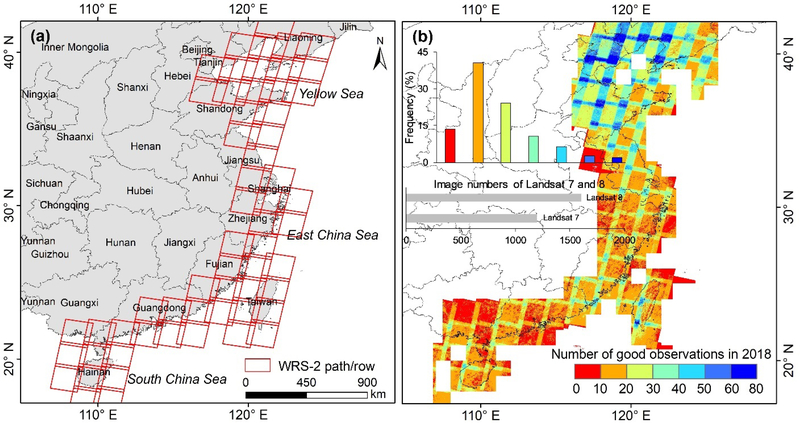
China’s coastline spans two municipalities (Shanghai and Tianjin), two special administrative regions (Macao and Hong Kong), and eleven provinces (Shandong, Liaoning, Hebei, Jiangsu, Fujian, Zhejiang, Guangxi Zhuang Autonomous Region, Hainan, Guangdong, and Taiwan) (Fig. 1a). Macao and Hong Kong have relatively small areas and are close to Guangdong Province, so we combined them as one region when we calculated coastal wetlands areas. We also didn’t include those islands in South China Sea in this study.
Fig. 1.
The spatial distribution of the coastal zone and Landsat WRS-2 path/rows in China (a) and the spatial distribution of the number of good-quality observations within individual pixels of Landsat 7/8 images in 2018 (b).
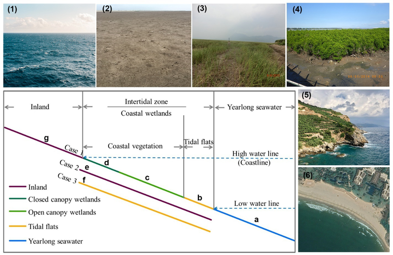
Coastal wetlands, also defined as intertidal flat ecosystems, include non-vegetated tidal flats (unconsolidated fine-grain sediments, unconsolidated coarse-grain sediments, consolidated sediments, organic materials or rocks) and vegetation-dominated intertidal ecosystems (e.g., mangroves and saltmarshes) (Murray et al., 2019). Furthermore, coastal vegetation types are usually composed of evergreen vegetation (e.g., closed-canopy mangroves) and deciduous vegetation (e.g., saltmarshes). Therefore, we divided the coastal wetlands into three types in this study: evergreen wetlands, deciduous wetlands, and non-vegetated tidal flats (Fig. 2). Paddy rice fields were excluded in this study.
Fig. 2.
An illustration of wetland types on the coastal zones in China. (a) Year-long sea water; (b) Non-vegetated tidal flats; (c) Open-canopy vegetation; (d) Closed-canopy vegetation; and (g) Inland. Coastal wetlands include tidal flats and coastal vegetation which comprise open and closed canopy wetlands. Case (1–3) show three types of coast zones in China. Case1: Common mud-deposited coastal wetlands; Case 2: Rocky coast without coastal wetlands; Case 3: Sandy coast without coastal vegetation. Subfigures (1–6) show the corresponding land cover photos of (a-f).
2.2. Data
2.2.1. Landsat data
China’s coastal zone covers 57 tiles (path/rows) of the Landsat Worldwide Reference System (WRS-2) (Fig. 1a). We processed all the available 2,444 Landsat surface reflectance images (1,046 Landsat 7 Surface Reflectance Tier 1, 1,398 Landsat 8 Surface Reflectance Tier 1) from January 1, 2015 to December 31, 2015 in GEE to generate the coastal wetland maps for 2015 for inter-comparison, and used 2,798 Landsat images (1,197 Landsat 7, 1,601 Landsat 8) from January 1, 2018 to December 31, 2018 to generate the coastal wetland maps for 2018 (Fig. 1b, Table S1). The Quality Assessment (QA) band flags bad-quality observations of each image (e.g. clouds and cloud shadows), and we used the QA band to remove bad-quality observations. In addition, we identified and removed terrain shadows using the Shuttle Radar Topography Mission (SRTM) digital elevation model (DEM) (Farr et al., 2007), the solar azimuth and zenith angles of each image, and the ee.Terrain.hillShadow algorithm in GEE (Zou et al., 2018). In China’s coastal zone, more than 87% (1,908 million) of the total pixels (2,207 million) had more than 10 good-quality observations in 2018, and most of North China had more than 50 good-quality observations due to the overlapping of Landsat images at the high latitudes and less cloud cover (Dong et al., 2016) (Fig. 1b).
In our study, we used four widely used spectral indices to identify surface water bodies and green vegetation: the Normalized Difference Vegetation Index (NDVI) (Tucker, 1979), Enhanced Vegetation Index (EVI) (Huete et al., 2002, 1997), Land Surface Water Index (LSWI) (Gao, 1996; Xiao, 2004), and the modified Normalized Difference Water Index (mNDWI) (Xu, 2006). NDVI and EVI are closely related to green vegetation (Wang et al., 2018), LSWI is a good indicator of vegetation and soil water (Xiao, 2004), and mNDWI is one of the most popular indices for mapping open surface water bodies. These indices are defined as:
| (1) |
| (2) |
| (3) |
| (4) |
where ρblue, ρgreen, ρred, ρnir, and ρswir are blue, green, red, near-infrared, and shortwave infrared bands of Landsat images.
2.2.2. Training datasets
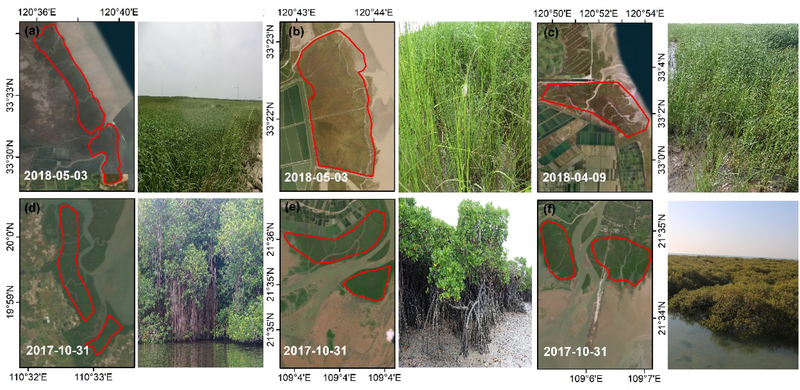
Compared to non-vegetated tidal flats, coastal vegetation often is relatively easy to visually interpret, so we selected 14 deciduous wetlands areas of interest (AOIs) (e.g. saltmarsh) and 8 evergreen wetlands AOIs (e.g. mangrove in South China) (Fig. 3) as training data and studied their distributions of water and vegetation signatures (see Fig. 6 for more details). All the training datasets were obtained from very high spatial resolution images available in Google Earth for algorithm development. When we draw these AOIs, small areas were delineated to reduce the inclusion of mixed pixels at the edge of the AOIs.
Fig. 3.
Location of areas of interest (AOIs) of coastal vegetation and the corresponding field photos. (a-c) AOIs of deciduous coastal wetlands; (d-f) AOIs of evergreen wetlands.
Fig. 6.
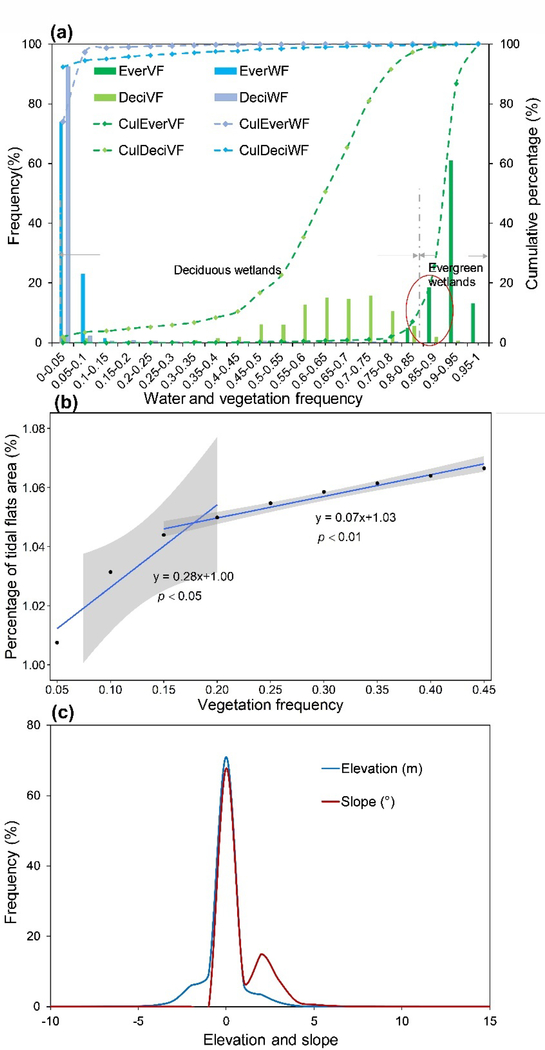
Indices distribution of coastal vegetation training area of interest (AOIs). (a) Distribution of vegetation frequency (VF) and water frequency (WF) of deciduous (DeciVF, DeciWF), evergreen wetlands (EverVF, EverWF), and their cumulative percentages; (b) Areas of tidal flats using different vegetation frequency thresholds; (c) Distribution of slope and elevation based on coastal vegetation training AOIs.
2.3. Coastal wetlands mapping algorithms
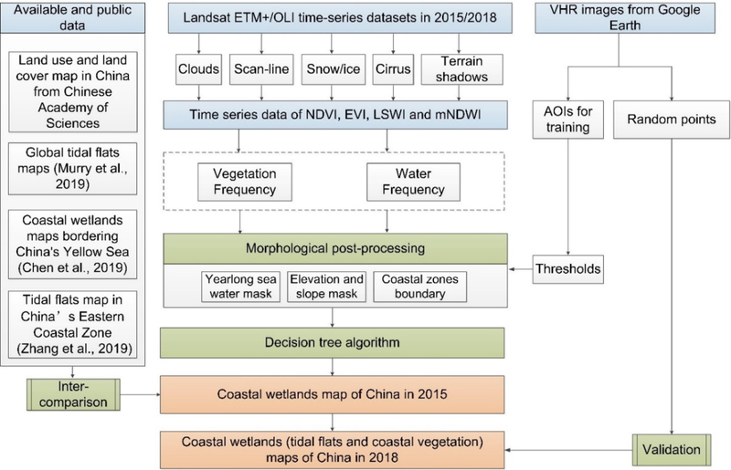
We developed a pixel- and phenology-based mapping algorithm for annual coastal wetland maps (Fig. 4). The algorithm was divided into three parts for each pixel: (1) identification of surface water body and green vegetation, (2) frequency estimates of surface water body and green vegetation, and (3) classification of coastal wetlands (including tidal flats and coastal vegetation). We implemented the algorithm for all good-quality observations to produce annual coastal wetland maps of China for 2015 and 2018 (see section 2.4).
Fig. 4.
Workflow for mapping China’s coastal wetlands.
2.3.1. Algorithm to identify surface water body and green vegetation per pixel
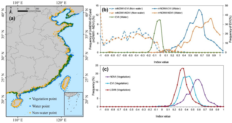
The mNDWI index has been widely used to identify open surface water bodies across different satellite sensors, including MODIS (Feng et al., 2012), Landsat (Pekel et al., 2016, 2014), and Sentinel-2 (Du et al., 2016). However, maps can have commission errors if pixels are mixed with vegetation (Santoro et al., 2015). For our study, we used a water detection algorithm (mNDWI/VIs), which combined mNDWI, NDVI, and EVI, to reduce the errors induced by vegetation when identifying surface water bodies (Wang et al., 2019; Zhou et al., 2019; Zou et al., 2018, 2017). For spectral signature analysis of land cover types, 30 water points and 25 non-water points were selected visually within each path/row tile based on the very high spatial resolution images of 2018 in the Google Earth. Altogether, a total of 1,710 water pixels and 1,425 non-water pixels were selected (Fig. 5a), and the distributions of the spectral indices were shown in Fig. 5b. We found that almost all the water pixels had mNDWI > EVI (99.10%) and mNDWI > NDVI (98.99%), and almost all the non-water pixels had mNDWI < EVI (97.13%) and mNDWI < NDVI (97.46%). Thus, we determined that mNDWI > EVI and mNDWI > NDVI were very good criteria to distinguish water from non-water points. In addition, almost all the water pixels had EVI < 0.1 (99.76%), thus EVI < 0.1 can be used to select the pure water pixels. The final water detection algorithm was ((mNDWI > EVI or mNDWI > NDVI) and EVI < 0.1). This mNDWI/VIs algorithm has been used to mapping surface water body at different scales with high accuracy (Wang et al., 2018; Zhou et al., 2019; Zou et al., 2018, 2017). In particular, a review paper described the differences of popular surface water detection algorithms (Zhou et al., 2017), and it found that the mNDWI/VIs algorithm can identify open surface water bodies in Landsat image with high accuracy (producer’s accuracy (98.1%) and user’s accuracy (91.0%)). Therefore, the mNDWI/VIs algorithm was used to identify open surface water bodies in this study.
Fig. 5.
Spectral characteristics of water, non-water, and vegetation sampling points. (a) Spatial distribution of vegetation and water sampling points; (b) mNDWI-EVI, mNDWI-NDVI, and EVI distributions of water and non-water points; (c) NDVI, EVI, and LSWI distributions of vegetation points.
NDVI and EVI are the most common indices used to detect vegetation and track their changes (Huete et al., 2002, 1997). However, water and soil can affect these vegetation indices and make vegetation identification difficult (Zou et al., 2018). LSWI is a good indicator to capture the signal of vegetation and soil water, so it can be used to identify dry (senescent) vegetation and soils that have a small amount of water (Xiao, 2004). Similarly, we randomly selected 1,425 points of vegetation in the coastal zone to study their distribution of different indices (NDVI, EVI, and LSWI) (Fig. 5c). We found that 96.82% of the vegetation pixels had NDVI values of ≥ 0.2, and 99.6% of the vegetation pixels had EVI values of ≥ 0.1. In addition, the LSWI values of all the vegetation pixels were greater than 0 (Fig. 5c). Therefore, we used (EVI ≥ 0.1, NDVI ≥ 0.2 and LSWI > 0) to map green vegetation in this study.
2.3.2. Frequency estimates of surface water body and green vegetation per pixel in a year
We determined the frequency of inundation to maximize the benefit of time series Landsat images and reduce the errors induced by bad-quality observations, periodical tidal, and in-completed phenological information of coastal vegetation. The water frequency (WF) of a pixel in a year was calculated as:
| (5) |
where WF is the water frequency ranged from 0 to 1, NWater is the number of water observations in a year, and NGood is the number of valid observations in a year. Similarly, we calculated the vegetation frequency (VF) as the ratio between the number of green vegetation observations (NVegetation) over the number of good-quality observations (NGood):
| (6) |
2.3.3. Algorithms to classify coastal wetlands per pixel
We used a simple land cover classification scheme with different WF and VF values: year-long seawater, tidal flats, and coastal vegetation (Fig. 2). Year-long seawater had a very steady state with a very high WF because of the less frequently affected by other factors (Wang et al., 2018; Zou et al., 2018), thus in our study 0.95 of WF was used as threshold to define the year-long seawater (WF ≥ 0.95) (Wang et al., 2018). From the histogram figure of VF and WF of coastal vegetation training AOIs (Fig. 6a), we found that almost all the evergreen vegetation had very high vegetation frequency (VF ≥ 0.90), so 0.90 of VF value can be used to identify evergreen and deciduous wetlands. We used a VF of 0.15 to differentiate tidal flats from deciduous wetlands, as Fig. 6b shows the sensitivity of tidal flats areas using different VF values, and the tidal flats area trend remained stable after VF increased from 0.05 to 0.15. In addition, we found that almost all the coastal vegetation pixels had −5 m < DEM < 5 m, and a slope < 5° (Fig. 6c), thus we used the rules DEM < 5 m and slope < 5 as a supplementary criterion to limit the boundary of coastal wetlands. In summary, the final mapping algorithms of tidal flats, deciduous wetlands, and evergreen wetlands were described using the following criteria:
| (7) |
| (8) |
| (9) |
2.4. Generation of coastal wetlands maps of China for 2015 and 2018
2.4.1. Potential region of coastal wetlands
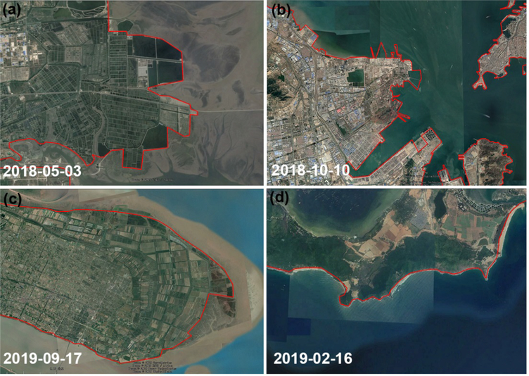
The natural coast of China could be divided into three types: rock, sand, and mud-deposition (Hou et al., 2016). It’s easy to identify the rock coasts as they have a clear boundary between land and seawater (Fig. 2e), but it is difficult to detect the distinct boundaries between sand or mud coasts and the mainland because the optical images cannot detect the high tidal waterline under dense vegetation (Chen et al., 2019). Fortunately, artificial shorelines, which formed by artificial buildings (e.g. aquaculture ponds, artificial engineering, artificial levee for reclamation and roads) and natural cliffs, can be used to separate the natural coastal wetlands from inland land cover types (Chen et al., 2019). As the artificial shorelines and natural cliffs can be easily recognized, we used simple visual interpretation method to delineate them in 2015 and 2018 at the scale of 1:24,000 using Google Earth (Fig. 7). Based on the artificial shorelines, we also created a 50-km buffer in marine environments as the potential natural coastal zone (Murray et al., 2019).
Fig. 7.
Main types of coastal shorelines.(a) Aquaculture ponds (32°14’35” N, 121°28’02” E); (b) Artificial engineering (36°03’21” N, 120 ° 13’35” E); (c) Artificial levee for reclamation and roads (31°29’29” N, 121 ° 57’56” E); (d) Rocky coast (18°22’41” N, 110°00’05” E).
2.4.2. Generating coastal wetland maps of China for 2015 and 2018
After defining the potential coastal wetland zone as described in section 2.4.1, we identified the classification type for each pixel according to the aforementioned algorithms (Eq. (7–9)). Then all the pixels with good-quality observations within potential coastal wetland zone were processed using the same algorithms. Finally, we generated the coastal wetland maps of China for 2015 and 2018 in GEE.
2.5. Validation of the China’s coastal wetland map for 2018
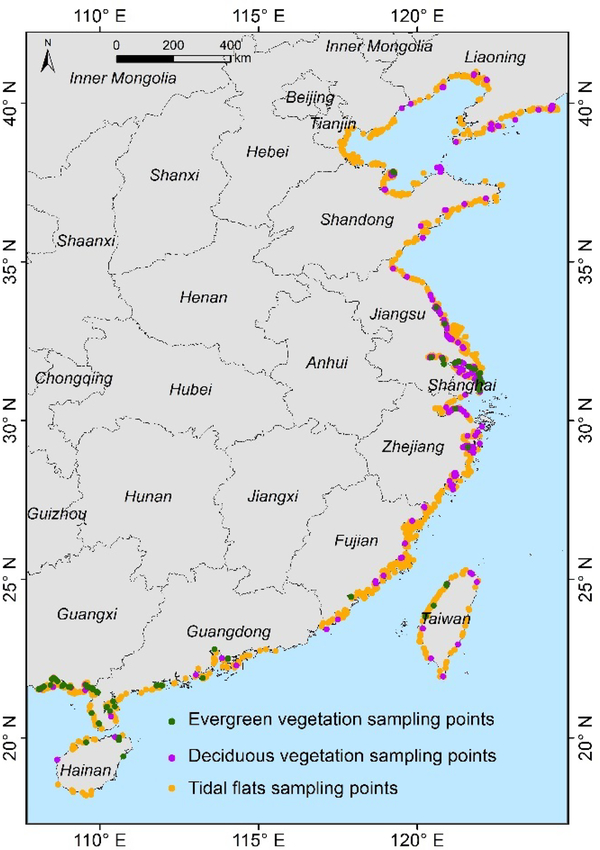
We used the stratified random sampling approach, which has been widely used in land cover validation (Chen et al., 2017; Murray et al., 2019; Pekel et al., 2016; Zou et al., 2018), to assess the accuracy of our coastal wetland map of China for 2018. First, coastal wetlands were partitioned into three classes (evergreen wetlands, deciduous wetlands, and tidal flats). Second, a total of 2,105 random sampling points (92 evergreen wetlands, 282 deciduous wetlands, and 1,723 tidal flats points (Fig. 8)) were generated using GEE’s random points function in each stratum within our resultant maps for 2018. Then, each of tidal flats (evergreen and deciduous) points was visually checked and interpreted in Google Earth. Its class was set as tidal flats or non-tidal flats land cover types (evergreen or non-evergreen, and deciduous or non-deciduous). Finally, we calculated the user’s accuracy, producer’s accuracy, overall accuracy, and Kappa coefficient (Table 3) after cross-checking between the random sampling points and very high spatial resolution images.
Fig. 8.
The distribution of random points for validation.
Table 3.
Confusion matrix of coastal wetlands validation for 2018.
| Ground reference pixels | Total | UA | ||||
|---|---|---|---|---|---|---|
| Class | Evergreen | Deciduous | Tidal flats | |||
| Map pixels | Evergreen | 88 | 1 | 3 | 92 | 95.7% |
| Deciduous | 4 | 266 | 12 | 282 | 94.3% | |
| Tidal flats | 0 | 23 | 1708 | 1731 | 98.7% | |
| Total | 92 | 290 | 1723 | 2105 | OA= 98.0% | |
| PA | 95.7% | 91.7% | 99.1% | K = 0.93 | ||
PA: Producer’s accuracy; UA: User’s accuracy; OA: Overall accuracy; K: Kappa coefficient
2.6. Comparison to other geospatial datasets of coastal wetlands in China
The 1-km land use and land cover (LULC) map of China for 2015 (LULC2015) was acquired from the Data Center for Resources and Environmental Sciences, Chinese Academy of Sciences (http://www.resdc.cn/data.aspx?DATAID=184). LULC2015 was generated using the visual interpretation of Landsat 8 images from 2015 and the 2010 LULC map. In the LULC2015 map, tidal flats were included in the water bodies class (Zhang et al., 2014). However, the classification system of the map didn’t include the coastal vegetation layer. Therefore, we compared the tidal flats areas from LULC2015 with the tidal flats areas that we identified in our coastal wetland maps in the same year (2015) which we have termed FUDAN/OU dataset.
Murray et al. (2019) at the University of Queensland (UQD) produced a global intertidal flats dataset (UQD dataset) by analyzing available Landsat satellite images in GEE platform during 1984–2016 and using the random forest algorithm for three-year time periods. For example, they generated one map named “2014–2016” using the Landsat dataset during 2014–2016. The definition of intertidal flats in UQD dataset was same with the definition in our study, so we compared our tidal flats map for 2015 to the UQD 2014–2016 map (available at https://www.intertidal.app/download).
In addition to the large-scale wetland datasets, some studies in China focused on coastal wetlands monitoring at regional scale. For example, Chen et al. (2019) completed the coastal wetlands maps (FAFU dataset) bordering China’s Yellow Sea during 1986–2015. Zhang et al. (2019) mapped coastal wetlands in the northern coastal zone of China for 2015 (SZU dataset) using the random forest algorithm. Thus, we compared our maps for 2015 to those acquired wetland maps in the same year.
3. Results
3.1. Accurate assessment of the annual map of coastal wetlands of China in 2018
The confusion matrix of the wetland map validation showed that our map of China for 2018 had high accuracy (Table 3). The overall accuracy of the resultant map was high (98.0%), and all accuracies including both producer’s accuracy (PA) and user’s accuracy (UA) were greater than 90.0%. The PA and UA of tidal flats were 98.7% and 99.1%, respectively, and they are higher than those of coastal vegetation. Deciduous wetlands had slightly lower accuracy among the three land cover types (UA 94.3% and PA 91.7%) because some deciduous points with very low vegetation frequency were regarded as tidal flats (see section 4.2 for more detail). The kappa coefficient of the validation was 0.93, and it indicated this study had a good agreement between mapped pixels and ground-referenced pixels.
3.2. Spatial distribution and areas of coastal wetlands of China in 2018
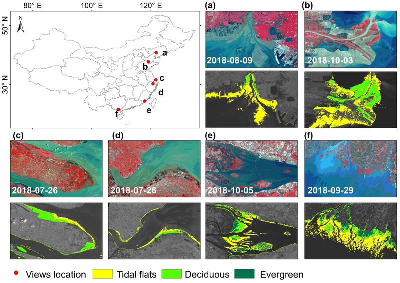
Fig. 9 shows the regional wetlands details in six typical bays and estuaries, and Table 4 shows the coastal wetland areas in each province of China in 2018. Total 7,474.6 km2 of coastal wetlands were found in China in 2018, which included 5,379.8 km2 of tidal flats, 1,856.4 km2 of deciduous wetlands, and 238.3 km2 of evergreen wetlands. Jiangsu Province had the largest wetlands area in China, followed by Shandong, Fujian, and Zhejiang Provinces. Tidal flats in China were mostly distributed along the coastlines of Jiangsu, Shandong, and Zhejiang Provinces. Jiangsu had the largest coastal vegetation area, followed by Shanghai, Zhejiang, and Shandong Provinces. Evergreen wetlands were mainly distributed in Guangdong and Guangxi Provinces, and deciduous wetlands were distributed in Jiangsu and Shanghai Provinces. Tianjin Province had the smallest wetlands area in China, as well as the smallest areas of tidal flats and coastal vegetation (Table 4). In addition, coastal wetlands in China mainly distributed in estuaries and bays, as well as Jiangsu Province (Fig. 9).
Fig. 9.
Regional subsets of coastal wetlands, showing the different distribution patterns of tidal flats, deciduous, evergreen wetlands, and Landsat RGB imagery. (a) Liao River Estuary; (b) Yellow River Estuary; (c) Yangtze River Estuary; (d) Hangzhou Bay; (e) Minjiang River Estuary; (f) Nanliu River Estuary.
Table 4.
Coastal wetlands areas (km2) in each province of China in 2018 as derived by our study.
| Province | Tidal flats | Deciduous | Evergreen | Coastal Vegetation (deciduous + evergreen) | Coastal wetlands (tidal flats + deciduous + evergreen) |
|---|---|---|---|---|---|
| Liaoning | 622.4 | 69.0 | 0.0 | 69.0 | 691.4 |
| Tianjin | 37.1 | 3.0 | 0.0 | 3.0 | 40.1 |
| Shandong | 823.2 | 228.3 | 1.2 | 229.5 | 1052.7 |
| Jiangsu | 1177.8 | 381.0 | 11.9 | 392.9 | 1570.7 |
| Fujian | 860.3 | 165.1 | 13.9 | 179.0 | 1039.3 |
| Guangdong | 329.8 | 113.2 | 70.1 | 183.3 | 513.1 |
| Guangxi | 300.1 | 133.9 | 51.7 | 185.6 | 485.7 |
| Hainan | 112.2 | 48.6 | 39.7 | 88.3 | 200.5 |
| Taiwan | 184.7 | 73.4 | 12.3 | 85.7 | 270.4 |
| Hebei | 144.2 | 10.1 | 0.0 | 10.1 | 154.3 |
| Zhejiang | 601.7 | 270.1 | 11.9 | 282.0 | 883.7 |
| Shanghai | 186.3 | 360.7 | 25.5 | 386.2 | 572.5 |
| Total | 5379.8 | 1856.4 | 238.3 | 2094.6 | 7474.4 |
3.3. Inter-comparison with other coastal wetlands maps or datasets
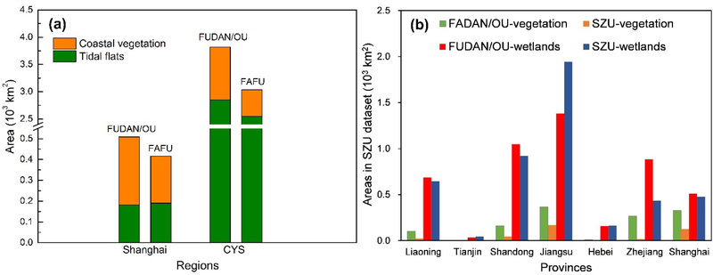
Recently, Chen et al. (2019) completed coastal wetland maps in the China’s Yellow Sea (CYS) for 2015 using time series Landsat images. In addition, they also reported the changes in coastal wetlands in Shanghai for 2015 (Chen et al., 2016). Thus, we got the coastal vegetation and tidal flats areas in Shanghai and CYS for 2015 from Chen’s studies (FAFU dataset) and compared them to our FUDAN/OU dataset for 2015 at the regional scale (Fig. 10a). The tidal flats in Shanghai were highly consistent between the two datasets, as FAFU reported the area to be 190 km2, and we determined the area to be 182 km2. However, we detected more coastal vegetation area in our dataset (327 km2) than the FAFU dataset (227 km2). In CYS, our FUDAN/OU dataset had 303 km2 more tidal flats and 480 km2 more coastal vegetation than the FAFU dataset. Different numbers of Landsat images in 2015, and different methods of detecting tidal flats and vegetation, contributed the larger areas of coastal wetlands in our study (see Discussion section for more detail).
Fig. 10.
Comparison of coastal wetland areas from our dataset (FUDAN/OU dataset) and other datasets in 2015. (a) Comparison between our study and the FAFU dataset (Chen et al., 2019, 2016); (b) Comparison between our study and the SZU dataset (Zhang et al., 2019).
Zhang et al. (2019) mapped coastal wetlands in the northern coastal zone of China in 2015 (SZU dataset) using the random forest algorithm. The total areas of coastal wetlands from the SZU dataset and our study matched very well, with 4,629.7 km2 and 4,704.8 km2, respectively. However, the SZU dataset detected much less vegetation (376.2 km2) than our study (1235.9 km2). At the provincial scale, we also detected more coastal wetlands and coastal vegetation than the SZU dataset (Fig. 10b). Different methods and different definitions of coastal zones were the main factors that caused the differences between the two studies (see Discussion section).
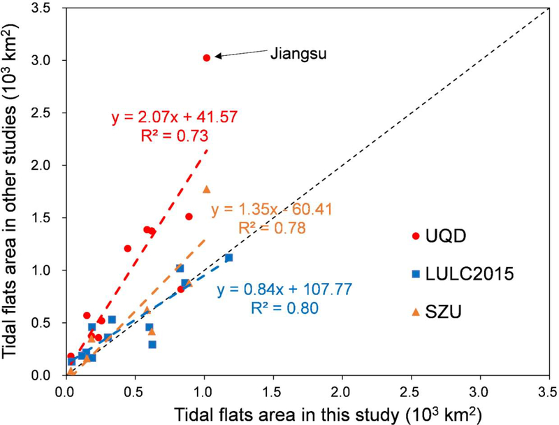
At the provincial scale, the tidal flats areas in our FUDAN/OU dataset matched well with the area of the LULC2015 and SZU datasets (Fig. 11). There are 5,836 km2 tidal flats of China in LULC2015, which was very close to the area from our dataset (5,342 km2). The tidal flats area in northern China in the SZU dataset was 3,959.9 km2, and in our dataset it was 3,468.9 km2. There were large differences in tidal flats areas between UQD and other datasets. The tidal flats area in the UQD dataset was 11,529 km2 but was 5,343 km2 in our study. Only Fujian Province had less tidal flats area in the UQD dataset than our FUDAN/OU dataset (Table 5).
Fig. 11.
Comparison of tidal flats areas in China between our dataset (FUDAN/OU) in 2015 and the UQD during 2014–2016 (Murray et al., 2019), the SZU in 2015 (Zhang et al., 2019), and the LULC2015 datasets.
Table 5.
Areas (km2) of tidal flats in China from our FUDAN/OU dataset in 2015 and the UQD during 2014–2016 (Murray et al., 2019), the SZU dataset in 2015 (Zhang et al., 2019), and the LULC2015 dataset.
| Province | UQD | SZU | LULC2015 | FUDAN/OU |
|---|---|---|---|---|
| Liaoning | 1388.2 | 624.4 | 293.0 | 584.5 |
| Tianjin | 182.0 | 44.9 | 131.0 | 32.4 |
| Shandong | 1512.7 | 879.1 | 1020.0 | 887.5 |
| Jiangsu | 3024.3 | 1774.1 | 1122.0 | 1016.2 |
| Hebei | 570.9 | 162.0 | 220.0 | 148.3 |
| Zhejiang | 1375.3 | 418.1 | 459.0 | 618.2 |
| Fujian | 819.4 | 882.0 | 829.7 | |
| Guangdong | 1208.4 | 532.0 | 443.9 | |
| Guangxi | 519.5 | 363.0 | 254.5 | |
| Hainan | 193.1 | 187.0 | 113.3 | |
| Taiwan | 360.4 | 461.0 | 232.3 | |
| Shanghai | 375.0 | 351.0 | 166.0 | 181.8 |
| Total | 11529.2 | 4253.4 | 5836.0 | 5342.7 |
4. Discussion
4.1. Annual maps of coastal wetlands of China at high spatial resolution
In this study we developed a pixel- and phenology-based algorithm for mapping coastal wetlands at 30-m spatial resolution in China’s coastal zone through analyses of time series Landsat images with Google Earth Engine platform, and the successful implementation of this study was attributed to the open access satellite data, simple but robust algorithm, and the powerful and user-friendly GEE platform. First, the open-access and free-availability of Landsat images have provided high temporal frequency of good-quality observations and can acquire the information of coastal wetlands effectively. Second, the pixel- and phenology-based algorithm maximized the Landsat images and could reduce the uncertainties induced from the bad-quality observations, periodical tide, and phenological information of coastal vegetation in the coastal zone. Third, GEE enables us to quickly acquire millions of Landsat images and process them in a paralleled way (Casu et al., 2017; Gorelick et al., 2017). Finally, we used the very-high spatial resolution images in Google Earth to interpret the artificial shorelines in China’s coastal zone and generated a 50-km buffer in the marine environment to define the potential regions of study area. This region could separate coastal wetlands from inland, remove the aquaculture ponds from coastal zone, and detect the outer boundary of tidal flats in the ocean clearly.
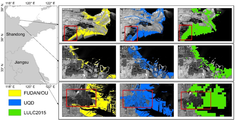
The comparison between our coastal wetland maps and other datasets and maps showed that there are some differences among these datasets (Fig. 10 and 11). Our dataset had 303 km2 more tidal flats area and 480 km2 more coastal vegetation area than the FAFU dataset in CYS (Chen et al., 2019), which can be mostly attributed to the different numbers of Landsat images and different detecting methods used to derive these two datasets. The Landsat Archive is gathering images from local stations around the world (https://landsat.usgs.gov/usgs-landsat-global-archive), and millions of images were added to Landsat Archive in GEE since the publication of the FAFU dataset in 2015 (Wulder et al., 2019, 2016). Thus, the increased in the number of Landsat images greatly increased the number of good-quality observations in China’s coastal zone and resulted in more coastal wetlands area being detected in our study than the FAFU dataset. In addition, we used a pixel- and phenology-based method to map coastal wetlands and combined NDVI, EVI, and LSWI to detect coastal vegetation (EVI ≥ 0.1, NDVI ≥ 0.2 and LSWI > 0), whereas the FAFU dataset used NDVI ≥ 0.1 to identify vegetation. These differences contributed the difference in the results reported by our study and the FAFU dataset. The different methods and different definitions of coastal zones used in our dataset and the SZU dataset resulted in the differences in coastal vegetation and tidal flats areas. The SZU dataset used the random forest algorithm, and our study used a pixel- and phenology-based algorithm. In addition, SZU used a 10 km landward buffer and a 40 km seaward buffer along the coastline as its study region, but we used a 50 km buffer from the artificial shoreline as our study region, which resulted in large difference in coastal vegetation area. The tidal flats area was highly consistent between our dataset and LULC2015 (Fig. 11). However, there are still some differences due to different methods used in these two datasets. In addition, the different spatial resolutions between our dataset (30 m) and the LULC2015 dataset (1 km) (http://www.resdc.cn/data.aspx?DATAID=184), also contributed to the differences in area derived by these two datasets (Fig. 12).
Fig. 12.
Three zoom-in views of tidal flats from our FUDAN/OU dataset in 2015, the UQD dataset during 2014–2016 (Murray et al., 2019), and the LULC2015 map in Shandong and Jiangsu Provinces of China.
Several reasons may explain the inconsistency between the UQD dataset and our FUDAN/OU dataset (Fig. 11). First, in terms of input image data, the UQD dataset used Landsat images during 2014–2016, and our FUDAN/OU dataset used images from 2015, thus the UQD dataset used much more Landsat data than our dataset. Second, in terms of the mapping algorithm, the UQD dataset used the random forest method, and we used a pixel- and phenology-based algorithm. Third, in terms of land cover classification scheme and definition, the UQD dataset detected nearly all the aquaculture ponds in the coastal zones as tidal flats (Fig. 12). As the aquaculture ponds in China’s coastal zone have expanded rapidly over the past three decades (Ren et al., 2019), the misclassification between aquaculture ponds and tidal flats caused an overestimation in the UQD dataset. In addition, regions where the near-infrared band mimicked the near-infrared band from tidal flats were identified as tidal flats in the UQD dataset (Fig. 13). However, the water frequency in these regions equaled one (Fig. 13c), and they were regarded as yearlong seawater in our dataset. Thus, the misclassification between yearlong seawater and tidal flats also contributed to the overestimation of tidal flats areas in UQD dataset. The inter-comparison between these datasets clearly suggests that there is a need to develop common validation dataset in the community, so that we can better characterize the effects of land cover classification scheme or definition, input datasets, and mapping algorithms on the accuracy and uncertainty of coastal wetland maps.
Fig. 13.
Spatial distribution of tidal flats and water frequency in the Yellow River Delta in 2015. (a) Spatial distribution of tidal flats from our FUDAN/OU dataset and the UQD dataset (Murray et al., 2019); (b) Spatial distribution of tidal flats from FUDAN/OU dataset and the location of area of interest (AOI); (c) Tidal flats in FUDAN/OU dataset, location of AOI, and the regions of water frequency was equal to 1. The background information of (a) and (b) is the band 5 (near-infrared band) of Landsat 8.
4.2. Potential sources of errors in the annual coastal wetland maps of China
The accuracy and uncertainty of resultant coastal wetland maps of China are affected by several factors, including input image data, in-situ training data, mapping algorithms, and land cover classification schemes or definitions. In this study, more than 87% of the pixels in 2018 had more than 10 good-quality observations (Fig. 1b), and the good-quality number of each pixel was enough to process the frequency-based algorithm to monitor the coastal wetlands. Nevertheless, the spatial inconsistency of the good-quality observations might still cause some uncertainties in the resultant coastal wetland maps (Wang et al., 2018). In addition, although most of bad-quality observations were removed by using the QA band (Zhu et al., 2015; Zhu and Woodcock, 2012), it’s impossible to remove all the bad-quality observations because of the limited quality of the QA band (Zou et al., 2018). Therefore, the bad-quality observations also could result in some inevitable uncertainties in the resultant maps.
Accurate location of shoreline is a factor that affects area summary report. As Landsat is sunsynchronous satellite and it has a 16-day repeat cycle, it is inevitable for us to only capture part of the full tidal range at a specific location (Dhanjal-Adams et al., 2016; Sagar et al., 2017). In addition, tidal variations within scenes also could bring some uncertainties on the coastal wetlands mapping (Wang et al., 2018). However, our pixel- and phenology-based method made use of all available Landsat images in GEE to reduce those impacts. A previous study reported that Landsat images can’t detect the high tidal line under the closed-canopy vegetations (Chen et al., 2019), and here we used visual interpretation to delineate the artificial shorelines and define the scope of coastal wetlands. But because of the limitation of visual interpretation, some isolated coastal vegetation, which have narrow connections to seawater, will be neglected, such as some mangrove forests in the southern China (Fig. 14a). Artificial shorelines also might increase the areas of coastal vegetation because some inland vegetation located between artificial shoreline and seawater were misidentified as coastal vegetation in this study. In addition, selecting training data based on visual interpretation also might bring few inevitable uncertainties on the resultant maps.
Fig. 14.
Illustration of typical uncertainties in our algorithm. (a) Isolated mangrove forests (21.679592° N, 108.859794° E); (b) Ephemeral vegetation which was regarded as tidal flats in 2018 (31.464716° N, 121.956125° E); (c) Field photo of ephemeral vegetation in 2018.
Mixed pixels of tidal flat and vegetation also affect the annual maps of coastal wetlands. The threshold of VF = 0.15 was used to detect the deciduous wetlands and tidal flats, so this threshold can cause mixture of tidal flats and deciduous wetlands when some coastal vegetations had very low VF in a specific year (0 < VF < 0.15). In fact, these sparse vegetations with low frequency were ephemeral plants and were regarded as tidal flats in this study referring to the detection methods (section 2.3, equation 7) (Fig. 14b and c). Fortunately, these ephemeral plants have very short lives and covered only a very small percentage of the total coastal wetlands in China.
4.3. Future implication and development of coastal wetlands mapping
The resultant coastal wetland maps of China for 2018 at 30-m spatial resolution are critical for better understanding of the detailed spatial information of coastal wetlands, as well as coastal vegetation and tidal flats in China, and can provide invaluable information for coastal sustainable management. The pixel- and phenology-based algorithm, time series Landsat images, and Google Earth Engine are useful in mapping annual coastal wetlands in China and could readily be applied to other regions in the world. This mapping strategy could be used to (1) track the dynamics of coastal wetlands in China over the past 3 decades (back to 1980s); and (2) monitor the global distribution and trajectory of coastal wetlands and serve as a more accurate coastal wetlands dataset than the previous global tidal flats dataset (Murray et al., 2019). However, this method may have significant errors when it is used in the tropical regions because of more frequent cloud cover (Dong et al., 2016). There are three strategies to reduce the errors in those regions with too many bad-quality observations. First, we can generate a coastal wetland map within each three-year timeperiod (such as, 2014–2016) through integrating all the available Landsat images during the period in GEE, which would greatly increase the number of good-quality observations. Second, we can integrate more optical satellite data at similar spatial resolutions with Landsat data, such as Sentinel-2 and Worldview 3, which have showed their potential for LULC mapping (Asadzadeh and de Souza Filho, 2016; Pahlevan et al., 2017; Puliti et al., 2018). Third, we can combine optical and microwave images to overcome the difficulties imposed by cloud cover and improve the accuracy of the resultant wetland maps. Microwave images from synthetic aperture radar (SAR), such as ALOS/ALOS-2 (Chen et al., 2018), ERS (Van Der Wal et al., 2005) and Sentinel-1 (Chen et al., 2017; Veloso et al., 2017), have become open access.
5. Conclusion
Previous efforts to map coastal wetlands have generally used visual interpretation, supervised, and unsupervised methods, and single-date or multi-date image mosaics (Table 1 and 2). However, the bad-quality observations, periodical tides, and in-completed phenological information of coastal vegetation in coastal zones make such classifications difficult and inaccurate. Accurate annual coastal wetland maps at large scales, which include tidal flats and coastal vegetation, have been very limited in China. We generated an unprecedented 30-m coastal wetland map of China for 2018 using a pixel- and phenology-based algorithm, the Landsat ETM+/OLI images in a single year, and the GEE platform. Our methods resulted in high producer’s and user’s accuracies, and the resultant maps have higher accuracies than the global tidal flats dataset (Murray et al., 2019). Therefore, the wetland maps in this study could serve as the newest dataset to support management and conservation of coastal wetlands in China with high accuracy.
Supplementary Material
Acknowledgements
This study was supported in part by research grants from the U.S. National Institutes of Health (1R01AI101028-02A1), the U.S. National Science Foundation (1911955), the National Natural Science Foundation of China (41601181, 41630528), and the China Scholarship Council (201906100124). We also thank the ISPRS editors and all the anonymous reviewers for their valuable comments and suggestions that helped us to improve this paper substantially.
Footnotes
Publisher's Disclaimer: This is a PDF file of an unedited manuscript that has been accepted for publication. As a service to our customers we are providing this early version of the manuscript. The manuscript will undergo copyediting, typesetting, and review of the resulting proof before it is published in its final form. Please note that during the production process errors may be discovered which could affect the content, and all legal disclaimers that apply to the journal pertain.
References
- Aiello-Lammens ME, Chu-Agor ML, Convertino M, Fischer RA, Linkov I, Resit Akçakaya H, 2011. The impact of sea-level rise on Snowy Plovers in Florida: Integrating geomorphological, habitat, and metapopulation models. Glob.Chang.Biol 17, 3644–3654. 10.1111/j.1365-2486.2011.02497.x [DOI] [Google Scholar]
- Amani M, Salehi B, Mahdavi S, Brisco B, 2018Spectral analysis of wetlands using multi-source optical satellite imagery. ISPRS J. Photogramm. Remote Sens 144, 119–136. 10.1016/j.isprsjprs.2018.07.005 [DOI] [Google Scholar]
- Arino O, Bicheron P, Achard F, Latham J, Witt R, Weber JL, 2008GLOBCOVER The most detailed portrait of Earth.Esa Bull. Sp. Agency 136, 25–31. [Google Scholar]
- Asadzadeh S, de Souza Filho CR, 2016Investigating the capability of WorldView-3 superspectral data for direct hydrocarbon detection. Remote Sens. Environ 173, 162–173. 10.1016/j.rse.2015.11.030 [DOI] [Google Scholar]
- Bansal S, Katyal D, Garg JK, 2017A novel strategy for wetland area extraction using multispectral MODIS data. Remote Sens. Environ 200, 183–205. 10.1016/j.rse.2017.07.034 [DOI] [Google Scholar]
- Bartholome E, Belward AS, 2005. GLC2000: a new approach to global land cover mapping from Earth observation data. Int. J. Remote Sens 26, 1959–1977. 10.1080/01431160412331291297 [DOI] [Google Scholar]
- Belgiu M, Csillik O, 2018Sentinel-2 cropland mapping using pixel-based and object-based time-weighted dynamic time warping analysis. Remote Sens. Environ 204, 509–523. 10.1016/j.rse.2017.10.005 [DOI] [Google Scholar]
- Bontemps JD, Hervé JC, Dhôte JF, 2010. Dominant radial and height growth reveal comparable historical variations for common beech in north-eastern France. For. Ecol. Manage 259, 1455–1463. 10.1016/j.foreco.2010.01.019 [DOI] [Google Scholar]
- Casu F, Manunta M, Agram PS, Crippen RE, 2017. Big Remotely Sensed Data: tools, applications and experiences. Remote Sens. Environ 202, 1–2. 10.1016/j.rse.2017.09.013 [DOI] [Google Scholar]
- Chen B, Xiao X, Ye H, Ma J, Doughty R, Li X, Zhao B, Wu Z, Sun R, Dong J, Qin Y, Xie G, 2018. Mapping Forest and Their Spatial-Temporal Changes From 2007 to 2015 in Tropical Hainan Island by Integrating ALOS/ALOS-2 L-Band SAR and Landsat Optical Images.Ieee J. Sel. Top. Appl. Earth Obs.Remote Sens. 11, 852–867. 10.1109/jstars.2018.2795595 [DOI] [Google Scholar]
- Chen BQ, Xiao XM, Li XP, Pan LH, Doughty R, Ma J, Dong JW, Qin YW, Zhao B, Wu ZX, Sun R, Lan GY, Xie GS, Clinton N, Giri C, 2017. A mangrove forest map of China in 2015: Analysis of time series Landsat 7/8 and Sentinel-1A imagery in Google Earth Engine cloud computing platform. ISPRS J. Photogramm. Remote Sens. 131, 104–120. 10.1016/j.isprsjprs.2017.07.011 [DOI] [Google Scholar]
- Chen Y, Dong J, Xiao X, Ma Z, Tan K, Melville D, Li B, Lu H, Liu J, Liu F, 2019Effects of reclamation and natural changes on coastal wetlands bordering China’s Yellow Sea from 1984 to 2015. L. Degrad. Dev 1–12. 10.1002/ldr.3322 [DOI] [Google Scholar]
- Chen Y, Dong JW, Xiao XM, Zhang M, Tian B, Zhou YX, Li B, Ma ZJ, 2016Land claim and loss of tidal flats in the Yangtze Estuary.Sci. Rep 6, 24018 10.1038/srep24018 [DOI] [PMC free article] [PubMed] [Google Scholar]
- Chu ZX, Sun XG, Zhai SK, Xu KH, 2006. Changing pattern of accretion/erosion of the modem Yellow River (Huanghe) subaerial delta, China: Based on remote sensing images. Mar. Geol 227, 13–30. 10.1016/j.margeo.2005.11.013 [DOI] [Google Scholar]
- Colomina I, Molina P, 2014. Unmanned aerial systems for photogrammetry and remote sensing: A review. ISPRS J. Photogramm. Remote Sens 92, 79–97. 10.1016/j.isprsjprs.2014.02.013 [DOI] [Google Scholar]
- Darby FA, Turner RE, 2008. Below- and aboveground Spartina alterniflora production in a Louisiana salt marsh. Estuaries and Coasts 31, 223–231. 10.1007/s12237-007-9014-7 [DOI] [Google Scholar]
- Davranche A, Lefebvre G, Poulin B, 2010. Wetland monitoring using classification trees and SPOT-5 seasonal time series. Remote Sens. Environ 114, 552–562. 10.1016/j.rse.2009.10.009 [DOI] [Google Scholar]
- Dhanjal-Adams KL, Hanson JO, Murray NJ, Phinn SR, Wingate VR, Mustin K, Lee JR, Allan JR, Cappadonna JL, Studds CE, Clemens RS, Roelfsema CM, Fuller RA, 2016. The distribution and protection of intertidal habitats in Australia.Emu 116, 208 [Google Scholar]
- Dong J, Xiao X, Menarguez MA, Zhang G, Qin Y, Thau D, Biradar C, Moore B, 2016Mapping paddy rice planting area in northeastern Asia with Landsat 8 images, phenology-based algorithm and Google Earth Engine. Remote Sens. Environ. 185, 142–154. 10.1016/j.rse.2016.02.016 [DOI] [PMC free article] [PubMed] [Google Scholar]
- Dronova I, Gong P, Wang L, Zhong LH, 2015. Mapping dynamic cover types in a large seasonally flooded wetland using extended principal component analysis and object-based classification. Remote Sens. Environ 158, 193–206. 10.1016/j.rse.2014.10.027 [DOI] [Google Scholar]
- Du Y, Zhang Y, Ling F, Wang Q, Li W, Li X, 2016Water bodies’ mapping from Sentinel-2 imagery with Modified Normalized Difference Water Index at 10-m spatial resolution produced by sharpening the swir band.Remote Sens. 8, 354 10.3390/rs8040354 [DOI] [Google Scholar]
- Ericson JP, Vörösmarty CJ, Dingman SL, Ward LG, Meybeck M, 2006. Effective sea-level rise and deltas: Causes of change and human dimension implications.Glob.Planet. Change 50, 63–82. 10.1016/j.gloplacha.2005.07.004 [DOI] [Google Scholar]
- Farr TG, Rosen PA, Caro E, Crippen R, Duren R, Hensley S, Kobrick M, Paller M, Rodriguez E, Roth L, Seal D, Shaffer S, Shimada J, Umland J, Werner M, Oskin M, Burbank D, Alsdorf DE, 2007. The shuttle radar topography mission. Rev. Geophys 45, RG2004 10.1029/2005RG000183 [DOI] [Google Scholar]
- Feng L, Hu CM, Chen XL, Cai XB, Tian LQ, Gan WX, 2012. Assessment of inundation changes of Poyang Lake using MODIS observations between 2000 and 2010. Remote Sens. Environ. 121, 80–92. 10.1016/j.rse.2012.01.014 [DOI] [Google Scholar]
- Friedl MA, McIver DK, Hodges JCF, Zhang XY, Muchoney D, Strahler AH, Woodcock CE, Gopal S, Schneider A, Cooper A, Baccini A, Gao F, Schaaf C, 2002. Global land cover mapping from MODIS: algorithms and early results. Remote Sens. Environ. 83, 287–302. 10.1016/S0034-4257(02)00078-0 [DOI] [Google Scholar]
- Friedl MA, Sulla-Menashe D, Tan B, Schneider A, Ramankutty N, Sibley A, Huang XM, 2010. MODIS Collection 5 global land cover: Algorithm refinements and characterization of new datasets. Remote Sens. Environ 114, 168–182. 10.1016/j.rse.2009.08.016 [DOI] [Google Scholar]
- Gao BC, 1996. NDWI - A normalized difference water index for remote sensing of vegetation liquid water from space. Remote Sens. Environ. 58, 257–266. 10.1016/s0034-4257(96)00067-3 [DOI] [Google Scholar]
- Ghosh S, Mishra DR, Gitelson AA, 2016Long-term monitoring of biophysical characteristics of tidal wetlands in the northern Gulf of Mexico - A methodological approach using MODIS. Remote Sens. Environ. 173, 39–58. 10.1016/j.rse.2015.11.015 [DOI] [Google Scholar]
- Gong P, Liu H, Zhang M, Li C, Wang J, Huang H, Clinton N, Ji L, Li W, Bai Y, Chen B, Xu B, Zhu Z, Yuan C, Ping Suen H, Guo J, Xu N, Li W, Zhao Y, Yang J, Yu C, Wang X, Fu H, Yu L, Dronova I, Hui F, Cheng X, Shi X, Xiao F, Liu Q, Song L, 2019. Stable classification with limited sample: transferring a 30-m resolution sample set collected in 2015 to mapping 10-m resolution global land cover in 2017. Sci. Bull. 64, 370–373. 10.1016/j.scib.2019.03.002 [DOI] [PubMed] [Google Scholar]
- Gong P, Niu ZG, Cheng XA, Zhao KY, Zhou DM, Guo JH, Liang L, Wang XF, Li DD, Huang HB, Wang Y, Wang K, Li WN, Wang XW, Ying Q, Yang ZZ, Ye YF, Li Z, Zhuang DF, Chi YB, Zhou HZ, Yan J, 2010. China’s wetland change (1990–2000) determined by remote sensing. Sci. China-Earth Sci 53, 1036–1042. 10.1007/s11430-010-4002-3 [DOI] [Google Scholar]
- Gong P, Wang J, Yu L, Zhao YC, Zhao YY, Liang L, Niu ZG, Huang XM, Fu HH, Liu S, Li CC, Li XY, Fu W, Liu CX, Xu Y, Wang XY, Cheng Q, Hu LY, Yao WB, Zhang H, Zhu P, Zhao ZY, Zhang HY, Zheng YM, Ji LY, Zhang YW, Chen H, Yan A, Guo JH, Yu L, Wang L, Liu XJ, Shi TT, Zhu MH, Chen YL, Yang GW, Tang P, Xu B, Giri C, Clinton N, Zhu ZL, Chen J, Chen J, 2013. Finer resolution observation and monitoring of global land cover: first mapping results with Landsat TM and ETM+ data. Int. J. Remote Sens 34, 2607–2654. 10.1080/01431161.2012.748992 [DOI] [Google Scholar]
- Gorelick N, Hancher M, Dixon M, Ilyushchenko S, Thau D, Moore R, 2017. Google Earth Engine: Planetary-scale geospatial analysis for everyone. Remote Sens. Environ 202, 18–27. 10.1016/j.rse.2017.06.031 [DOI] [Google Scholar]
- Han Q, Niu Z, Wu M, Wang J, 2019Remote-sensing monitoring and analysis of China intertidal zone changes based on tidal correction.Chinese Sci. Bull 64, 456–473. 10.1360/N972018-00723 [DOI] [Google Scholar]
- Hansen MC, Defries RS, Townshend JRG, Sohlberg R, 2000. Global land cover classification at 1km spatial resolution using a classification tree approach. Int. J. Remote Sens 21, 1331–1364. 10.1080/014311600210209 [DOI] [Google Scholar]
- Held A, Ticehurst C, Lymburner L, Williams N, 2003High resolution mapping of tropical mangrove ecosystems using hyperspectral and radar remote sensing. Int. J. Remote Sens. 24, 2739–2759. 10.1080/0143116031000066323 [DOI] [Google Scholar]
- Hodoki Y, Murakami T, 2006Effects of tidal flat reclamation on sediment quality and hypoxia in Isahaya Bay. Aquat.Conserv.Freshw.Ecosyst 16, 555–567. 10.1002/aqc.723 [DOI] [Google Scholar]
- Hou XY, Wu T, Hou W, Chen Q, Wang YD, Yu LJ, 2016Characteristics of coastline changes in mainland China since the early 1940s. Sci. China Earth Sci 59, 1791–1802. 10.1007/s11430-016-5317-5 [DOI] [Google Scholar]
- Huete A, Didan K, Miura T, Rodriguez EP, Gao X, Ferreira LG, 2002. Overview of the radiometric and biophysical performance of the MODIS vegetation indices. Remote Sens. Environ 83, 195–213. 10.1016/s0034-4257(02)00096-2 [DOI] [Google Scholar]
- Huete AR, Liu HQ, Batchily K, vanLeeuwen W, 1997. A comparison of vegetation indices global set of TM images for EOS-MODIS. Remote Sens. Environ 59, 440–451. 10.1016/s0034-4257(96)00112-5 [DOI] [Google Scholar]
- Jia M, Wang Z, Zhang Y, Mao D, Wang C, 2018Monitoring loss and recovery of mangrove forests during 42 years: The achievements of mangrove conservation in China.Int. J. Appl. Earth Obs. Geoinf 73, 535–545. 10.1016/j.jag.2018.07.025 [DOI] [Google Scholar]
- Jung R, Adolph W, Ehlers M, Farke H, 2015. A multi-sensor approach for detecting the different land covers of tidal flats in the German Wadden Sea - A case study at Norderney. Remote Sens. Environ 170, 188–202. 10.1016/j.rse.2015.09.018 [DOI] [Google Scholar]
- Kim DJ, Moon WM, Kim G, Park SE, Lee H, 2011. Submarine groundwater discharge in tidal flats revealed by space-borne synthetic aperture radar. Remote Sens. Environ 115, 793–800. 10.1016/j.rse.2010.11.009 [DOI] [Google Scholar]
- Kou W, Dong J, Xiao X, Hernandez AJ, Qin Y, Zhang G, Chen B, Lu N, Doughty R, 2018Expansion dynamics of deciduous rubber plantations in Xishuangbanna, China during 2000–2010.GIScience Remote Sens. 55, 905–925. 10.1080/15481603.2018.1466441 [DOI] [Google Scholar]
- Li WY, Gong P, 2016. Continuous monitoring of coastline dynamics in western Florida with a 30-year time series of Landsat imagery. Remote Sens. Environ 179, 196–209. 10.1016/j.rse.2016.03.031 [DOI] [Google Scholar]
- Liu M, Mao D, Wang Z, Li L, Man W, Jia M, Ren C, Zhang Y, 2018. Rapid invasion of Spartina alterniflora in the coastal zone of mainland China: New observations from Landsat OLI images. Remote Sens.10, 1933 10.3390/rs10121933 [DOI] [PMC free article] [PubMed] [Google Scholar]
- Liu T, Abd-Elrahman A, 2018Deep convolutional neural network training enrichment using multi-view object-based analysis of Unmanned Aerial systems imagery for wetlands classification. ISPRS J. Photogramm. Remote Sens 139, 154–170. 10.1016/j.isprsjprs.2018.03.006 [DOI] [Google Scholar]
- Loveland TR, Reed BC, Brown JF, Ohlen DO, Zhu Z, Yang L, Merchant JW, 2000. Development of a global land cover characteristics database and IGBP DISCover from 1 km AVHRR data. Int. J. Remote Sens 21, 1303–1330. 10.1080/014311600210191 [DOI] [Google Scholar]
- Ma T, Li X, Bai J, Cui B, 2019. Tracking three decades of land use and land cover transformation trajectories in China’s large river deltas. L. Degrad. Dev 30, 799–810. 10.1002/ldr.3268 [DOI] [Google Scholar]
- Ma ZJ, Hua N, Peng HB, Choi C, Battley PF, Zhou QY, Chen Y, Ma Q, Jia N, Xue WJ, Bai QQ, Wu W, Feng XS, Tang CD, 2013. Differentiating between stopover and staging sites: functions of the southern and northern Yellow Sea for long-distance migratory shorebirds. J. Avian Biol 44, 504–512. 10.1111/j.1600-048X.2013.00213.x [DOI] [Google Scholar]
- Ma ZJ, Melville DS, Liu JG, Chen Y, Yang HY, Ren WW, Zhang ZW, Piersma T, Li B, 2014ECOSYSTEMS MANAGEMENT Rethinking China’s new great wall.Science. 346, 912–914. 10.1126/science.1257258 [DOI] [PubMed] [Google Scholar]
- Mohammadimanesh F, Salehi B, Mahdianpari M, Brisco B, Motagh M, 2018. Multi-temporal, multifrequency, and multi-polarization coherence and SAR backscatter analysis of wetlands. ISPRS J. Photogramm. Remote Sens 142, 78–93. 10.1016/j.isprsjprs.2018.05.009 [DOI] [Google Scholar]
- Morris JT, Sundareshwar PV, Nietch CT, Kjerfve B, Cahoon DR, 2002. Responses of coastal wetlands to rising sea level.Ecology 83, 2869–2877. 10.2307/3072022 [DOI] [Google Scholar]
- Murray NJ, Clemens RS, Phinn SR, Possingham HP, Fuller RA, 2014Tracking the rapid loss of tidal wetlands in the Yellow Sea. Front. Ecol. Environ 12, 267–272. 10.1890/130260 [DOI] [Google Scholar]
- Murray NJ, Phinn SR, Clemens RS, Roelfsema CM, Fuller RA, 2012. Continental scale mapping of tidal flats across east Asia using the landsat archive. Remote Sens. 4, 3417–3426. 10.3390/rs4113417 [DOI] [Google Scholar]
- Murray NJ, Phinn SR, DeWitt M, Ferrari R, Johnston R, Lyons MB, Clinton N, Thau D, Fuller RA,2019. The global distribution and trajectory of tidal flats. Nature 565, 222 10.1038/s41586-018-0805-8 [DOI] [PubMed] [Google Scholar]
- Nicholls RJ, Cazenave A, 2010. Sea-level rise and its impact on coastal zones.Science. 328, 1517–1520. 10.1126/science.1185782 [DOI] [PubMed] [Google Scholar]
- Nielsen EM, Prince SD, Koeln GT, 2008. Wetland change mapping for the US mid-Atlantic region using an outlier detection technique. Remote Sens. Environ 112, 4061–4074. 10.1016/j.rse.2008.04.017 [DOI] [Google Scholar]
- Niu Z, Gong P, Cheng X, Guo J, Wang L, Huang H, Shen S, Wu Y, Wang X, Wang X, Ying Q, Liang L, Zhang L, Wang L, Yao Q, Yang Z, Guo Z, Dai Y, 2009. Geographical characteristics of China’s wetlands derived from remotely sensed data. Sci. China Ser. D-Earth Sci 52, 723–738. 10.1007/s11430-009-0075-2 [DOI] [Google Scholar]
- Niu Z, Zhang H, Wang X, Yao W, Zhou D, Zhao K, Zhao H, Li N, Huang H, Li C, Yang J, Liu C, Liu S, Wang L, Li Z, Yang Z, Qiao F, Zheng Y, Chen Y, Sheng Y, Gao X, Zhu W, Wang W, Wang H, Weng Y, Zhuang D, Liu J, Luo Z, Cheng X, Guo Z, Gong P, 2012. Mapping wetland changes in China between 1978 and 2008.Chinese Sci. Bull 57, 2813–2823. 10.1007/s11434-012-5093-3 [DOI] [Google Scholar]
- Oost AP, Hoekstra P, Wiersma A, Flemming B, Lammerts EJ, Pejrup M, Hofstede J, van der Valk B, Kiden P, Bartholdy J, van der Berg MW, Vos PC, de Vries S, Wang ZB, 2012. Barrier island management: Lessons from the past and directions for the future. Ocean Coast.Manag 68, 18–38. 10.1016/j.ocecoaman.2012.07.010 [DOI] [Google Scholar]
- Pahlevan N, Sarkar S, Franz BA, Balasubramanian SV, He J, 2017. Sentinel-2 MultiSpectral Instrument (MSI) data processing for aquatic science applications: Demonstrations and validations. Remote Sens.Environ. 201, 47–56. 10.1016/j.rse.2017.08.033 [DOI] [Google Scholar]
- Pekel JF, Cottam A, Gorelick N, Belward AS, 2016. High-resolution mapping of global surface water and its long-term changes.Nature 540, 418 10.1038/nature20584 [DOI] [PubMed] [Google Scholar]
- Pekel JF, Vancutsem C, Bastin L, Clerici M, Vanbogaert E, Bartholomé E, Defourny P, 2014. A near real-time water surface detection method based on HSV transformation of MODIS multi-Spectral time series data. Remote Sens. Environ 140, 704–716. 10.1016/j.rse.2013.10.008 [DOI] [Google Scholar]
- Puliti S, Saarela S, Gobakken T, Ståhl G, Næsset E, 2018. Combining UAV and Sentinel-2 auxiliary data for forest growing stock volume estimation through hierarchical model-based inference. Remote Sens. Environ 204, 485–497. 10.1016/j.rse.2017.10.007 [DOI] [Google Scholar]
- Ren C, Wang Z, Zhang Y, Zhang B, Chen L, Xi Y, Xiao X, Doughty RB, Liu M, Jia M, Mao D,Song K, 2019. Rapid expansion of coastal aquaculture ponds in China from Landsat observations during 1984–2016.Int. J. Appl. Earth Obs. Geoinf 82, 101902 10.1016/J.JAG.2019.101902 [DOI] [Google Scholar]
- Rodriguez JF, Saco PM, Sandi S, Saintilan N, Riccardi G, 2017. Potential increase in coastal wetland vulnerability to sea-level rise suggested by considering hydrodynamic attenuation effects. Nat. Commun 8, 16094 [DOI] [PMC free article] [PubMed] [Google Scholar]
- Sagar S, Roberts D, Bala B, Lymburner L, 2017. Extracting the intertidal extent and topography of the Australian coastline from a 28 year time series of Landsat observations. Remote Sens. Environ 195, 153–169. 10.1016/j.rse.2017.04.009 [DOI] [Google Scholar]
- Santoro M, Wegmueller U, Lamarche C, Bontemps S, Defoumy P, Arino O, 2015. Strengths and weaknesses of multi-year Envisat ASAR backscatter measurements to map permanent open water bodies at global scale. Remote Sens. Environ 171, 185–201. 10.1016/j.rse.2015.10.031 [DOI] [Google Scholar]
- Seto KC, Fragkias M, 2007. Mangrove conversion and aquaculture development in Vietnam: A remote sensing-based approach for evaluating the Ramsar Convention on Wetlands. Glob. Environ. Chang 17, 486–500. 10.1016/j.gloenvcha.2007.03.001 [DOI] [Google Scholar]
- Simard M, De Grandi G, Saatchi S, Mayaux P, 2002. Mapping tropical coastal vegetation using JERS-1 and ERS-1 radar data with a decision tree classifier. Int. J. Remote Sens 23, 1461–1474. 10.1080/01431160110092984 [DOI] [Google Scholar]
- Tucker CJ, 1979. Red and photographic infrared linear combinations for monitoring vegetation.Remote Sens.Environ 8, 127–150. 10.1016/0034-4257(79)90013-0 [DOI] [Google Scholar]
- Van Der Wal D, Herman PMJ, Wielemaker-Van Den Dool A, 2005. Characterisation of surface roughness and sediment texture of intertidal flats using ERS SAR imagery. Remote Sens. Environ 98, 96–109. 10.1016/j.rse.2005.06.004 [DOI] [Google Scholar]
- Veloso A, Mermoz S, Bouvet A, Le Toan T, Planells M, Dejoux JF, Ceschia E, 2017Understanding the temporal behavior of crops using Sentinel-1 and Sentinel-2-like data for agricultural applications. Remote Sens. Environ 199, 415–426. 10.1016/j.rse.2017.07.015 [DOI] [Google Scholar]
- Wang J, Niu Z, 2017. Remote-sensing analysis of Yancheng intertidal zones based on tidal correction. Haiyang Xuebao 39, 149–160. 10.3969/j.issn.0253-4193.2017.05.014 [DOI] [Google Scholar]
- Wang X, Xiao X, Zou Z, Chen B, Ma J, Dong J, Doughty RB, Zhong Q, Qin Y, Dai S, Li X, Zhao B, Li B, Qiaoyan Z, Qin Y, Dai S, Li X, Zhao B, Li B, 2018Tracking annual changes of coastal tidal flats in China during 1986–2016 through analyses of Landsat images with Google Earth Engine. Remote Sens. Environ 110987 [DOI] [PMC free article] [PubMed] [Google Scholar]
- Wang Y, Ma J, Xiao X, Wang X, Dai S, Zhao B, 2019. Long-Term Dynamic of Poyang Lake Surface Water: A Mapping Work Based on the Google Earth Engine Cloud Platform.Remote Sens. 11, 313 10.3390/rs11030313 [DOI] [Google Scholar]
- Wu W, Zhou Y, Tian B, 2017. Coastal wetlands facing climate change and anthropogenic activities: A remote sensing analysis and modelling application. Ocean Coast.Manag 138, 1–10. 10.1016/j.ocecoaman.2017.01.005 [DOI] [Google Scholar]
- Wulder MA, Loveland TR, Roy DP, Crawford CJ, Masek JG, Woodcock CE, Allen RG, Anderson MC, Belward AS, Cohen WB, Dwyer J, Erb A, Gao F, Griffiths P, Helder D, Hermosilla T, Hipple JD, Hostert P, Hughes MJ, Huntington J, Johnson DM, Kennedy R, Kilic A, Li Z, Lymburner L, McCorkel J, Pahlevan N, Scambos TA, Schaaf C, Schott JR, Sheng Y, Storey J, Vermote E, Vogelmann J, White JC, Wynne RH, Zhu Z, 2019. Current status of Landsat program, science, and applications. Remote Sens. Environ 225, 127–147. 10.1016/j.rse.2019.02.015 [DOI] [Google Scholar]
- Wulder MA, White JC, Loveland TR, Woodcock CE, Belward AS, Cohen WB, Fosnight EA, Shaw J, Masek JG, Roy DP, 2016. The global Landsat archive: Status, consolidation, and direction. Remote Sens. Environ 185, 271–283. 10.1016/j.rse.2015.11.032 [DOI] [Google Scholar]
- Xiao X, 2004Modeling gross primary production of temperate deciduous broadleaf forest using satellite images and climate data. Remote Sens. Environ. 91, 256–270. 10.1016/j.rse.2004.03.010 [DOI] [Google Scholar]
- Xie C, Xu J, Shao Y, Cui B, Goel K, Zhang Y, Yuan M, 2015. Long term detection of water depth changes of coastal wetlands in the Yellow River Delta based on distributed scatterer interferometry. Remote Sens. Environ 164, 238–253. 10.1016/j.rse.2015.04.010 [DOI] [Google Scholar]
- Xu HQ, 2006. Modification of normalised difference water index (NDWI) to enhance open water features in remotely sensed imagery. Int. J. Remote Sens 27, 3025–3033. 10.1080/01431160600589179 [DOI] [Google Scholar]
- Yan F, Liu X, Chen J, Yu L, Yang C, Chang L, Yang J, Zhang S, 2017. China’s Wetland Databases Based on Remote Sensing Technology. Chinese Geogr. Sci 27, 374–388. 10.1007/s11769-017-0872-z [DOI] [Google Scholar]
- Yim J, Kwon BO, Nam J, Hwang JH, Choi K, Khim JS, 2018. Analysis of forty years long changes in coastal land use and land cover of the Yellow Sea: The gains or losses in ecosystem services. Environ. Pollut 241, 74–84. 10.1016/j.envpol.2018.05.058 [DOI] [PubMed] [Google Scholar]
- Zhang D, Liu G, Hu W, 2019. Mapping Tidal Flats with Landsat 8 Images and Google Earth Engine: A Case Study of the China’s Eastern Coastal Zone circa 2015. Remote Sens. 11, 924 10.3390/rs11080924 [DOI] [Google Scholar]
- Zhang Z, Wang X, Zhao X, Liu B, Yi L, Zuo L, Wen Q, Liu F, Xu J, Hu S, 2014. A 2010 update of National Land Use/Cover Database of China at 1:100000 scale using medium spatial resolution satellite images. Remote Sens. Environ 149, 142–154. 10.1016/J.RSE.2014.04.004 [DOI] [Google Scholar]
- Zhao B, Guo H, Yan Y, Wang Q, Li B, 2008. A simple waterline approach for tidelands using multi-temporal satellite images: A case study in the Yangtze Delta. Estuar.Coast. Shelf Sci 77, 134–142. 10.1016/j.ecss.2007.09.022 [DOI] [Google Scholar]
- Zhou Y, Dong J, Xiao X, Liu R, Zou Z, Zhao G, Ge Q, 2019Continuous monitoring of lake dynamics on the Mongolian Plateau using all available Landsat imagery and Google Earth Engine. Sci. Total Environ 689, 366–380. 10.1016/J.SCITOTENV.2019.06.341 [DOI] [PubMed] [Google Scholar]
- Zhou Y, Dong J, Xiao X, Xiao T, Yang Z, Zhao G, Zou Z, Qin Y, 2017. Open surface water mapping algorithms: A comparison of water-related spectral indices and sensors. Water 9, 256 10.3390/w9040256 [DOI] [Google Scholar]
- Zhu X, Hou Y, Weng Q, Chen L, 2019Integrating UAV optical imagery and LiDAR data for assessing the spatial relationship between mangrove and inundation across a subtropical estuarine wetland. ISPRS J. Photogramm. Remote Sens 149, 146–156. 10.1016/j.isprsjprs.2019.01.021 [DOI] [Google Scholar]
- Zhu Z, Wang S, Woodcock CE, 2015. Improvement and expansion of the Fmask algorithm: Cloud, cloud shadow, and snow detection for Landsats 4–7, 8, and Sentinel 2 images. Remote Sens. Environ 159, 269–277. 10.1016/j.rse.2014.12.014 [DOI] [Google Scholar]
- Zhu Z, Woodcock CE, 2012. Object-based cloud and cloud shadow detection in Landsat imagery. Remote Sens.Environ 118, 83–94. 10.1016/j.rse.2011.10.028 [DOI] [Google Scholar]
- Zhu Z, Wulder MA, Roy DP, Woodcock CE, Hansen MC, Radeloff VC, Healey SP, Schaaf C, Hostert P, Strobl P, Pekel JF, Lymburner L, Pahlevan N, Scambos TA, 2019a. Benefits of the free and open Landsat data policy. Remote Sens. Environ 224, 382–385. 10.1016/j.rse.2019.02.016 [DOI] [Google Scholar]
- Zhu Z, Zhang J, Yang Z, Aljaddani AH, 2019b. Continuous monitoring of land disturbance based on Landsat time series. Remote Sens. Environ 238, 111116 10.1016/j.rse.2019.03.009 [DOI] [Google Scholar]
- Zou ZH, Dong JW, Menarguez MA, Xiao XM, Qin YW, Doughty RB, Hooker KV, Hambright KD, 2017. Continued decrease of open surface water body area in Oklahoma during 1984–2015. Sci. Total Environ 595, 451–460. 10.1016/j.scitotenv.2017.03.259 [DOI] [PubMed] [Google Scholar]
- Zou ZH, Xiao XM, Dong JW, Qin YW, Doughty RB, Menarguez MA, Zhang GL, Wang J, 2018. Divergent trends of open-surface water body area in the contiguous United States from 1984 to 2016. Proc. Natl. Acad. Sci. U. S. A 115, 3810–3815. 10.1073/pnas.1719275115 [DOI] [PMC free article] [PubMed] [Google Scholar]
Associated Data
This section collects any data citations, data availability statements, or supplementary materials included in this article.


