

Abstract
We examined the effect of estimation methods, maximum likelihood (ML), unweighted least squares (ULS), and diagonally weighted least squares (DWLS), on three population SEM (structural equation modeling) fit indices: the root mean square error of approximation (RMSEA), the comparative fit index (CFI), and the standardized root mean square residual (SRMR). We considered different types and levels of misspecification in factor analysis models: misspecified dimensionality, omitting cross-loadings, and ignoring residual correlations. Estimation methods had substantial impacts on the RMSEA and CFI so that different cutoff values need to be employed for different estimators. In contrast, SRMR is robust to the method used to estimate the model parameters. The same criterion can be applied at the population level when using the SRMR to evaluate model fit, regardless of the choice of estimation method.
Keywords: structural equation modeling (SEM), fit indices, estimation methods, close fit
In many applications of structural equation modeling (SEM), the model under consideration is to some degree misspecified, or in more plain terms, incorrect (Box, 1979; MacCallum, 2003). In these situations, it is of interest whether the model fits closely or, more precisely, whether the misfit is substantively ignorable (Shi, Maydeu-Olivares, & DiStefano, 2018). A host of goodness-of-fit indices have been developed in an attempt to assess the size of a model’s misfit. As MacCallum, Browne, and Sugawara (1996) put it,
If the model is truly a good model in terms of its fit in the population, we wish to avoid concluding that the model is a bad one. Alternatively, if the model is truly a bad one, we wish to avoid concluding that it is a good one. (p. 131)
However, in reality, the goodness-of-fit indices reflect not just the “size” of model misspecification in the population. Rather, fit indices can be influenced by other variables that are unrelated to the level of the model misfit (Saris, Satorra, & van der Veld, 2009).
One of these variables is the choice of estimation method (Beauducel & Herzberg, 2006; Savalei, 2017; Xia & Yang, 2019). When fitting SEM models with continuous outcomes, maximum likelihood (ML) is the most commonly used estimation method (Jöreskog, 1969; Maydeu-Olivares, 2017b). On the other hand, when the data are ordinal, estimators based on least squares, such as the unweighted least squares (ULS) and diagonally weighted least squares (DWLS) are generally recommended when ordinal data are present1 (Forero, Maydeu-Olivares, & Gallardo-Pujol, 2009; Jöreskog & Sörbom, 1988; Muthén, 1993; Muthén, du Toit, & Spisic, 1997; Savalei & Rhemtulla, 2013; Shi, DiStefano, McDaniel, & Jiang, 2018).
Understanding the effect of estimation methods on SEM fit indices is important when fitting SEM models to ordinal data for two reasons. First, conclusions and conventional cutoffs obtained using an estimator cannot be generalized to applications in which a different estimator has been used. Most previous studies on SEM fit indices used ML estimation, and conclusions and conventional cutoffs obtained using ML with continuous data (e.g., Hu & Bentler, 1999) cannot be generalized to situations where categorical estimation methods (e.g., ULS and DWLS) are used. Second, a number of studies (DiStefano & Morgan, 2014; Maydeu-Olivares, Cai, & Hernández, 2011; Rhemtulla, Brosseau-Liard, & Savalei, 2012) suggest that ordinal data with a large number of response categories (five or more categories) can be treated approximately as continuous. In these situations, using ML estimation when treating data as continuous or least squares methods when treating the data as ordinal will lead to substantially different fit indices across estimators, even when the same structural model is fitted to the data.2
Previous studies (e.g., Beauducel & Herzberg, 2006; Savalei, 2017; Xia & Yang, 2019) have examined the impact of estimation methods on SEM fit indices. In particular, a recent study by Xia and Yang (2019, see also Xia, 2016) has systematically examined the behavior of the root mean square error of approximation (RMSEA; Steiger, 1989, 1990; Steiger & Lind, 1980) and the comparative fit index (CFI; Bentler, 1990) across estimation methods. Using simulation and empirical examples, these authors found that DWLS and ULS consistently yield smaller RMSEA and larger CFI than those obtained using ML, suggesting that the model fits better. The above pattern held at both the population and sample levels. Based on the findings, the authors concluded that the RMSEA and CFI tell different stories depending on the estimation method; the ML-based conventional cutoffs should not be applied under categorical estimators.
However, Xia and Yang (2019) did not consider in their study goodness-of-fit indices that may be unaffected by the choice of estimator, such as the standardized root mean square residual (SRMR; Bentler, 1995; Jöreskog & Sörbom, 1988; Maydeu-Olivares, 2017a). The SRMR depends solely on the parameter estimates, and not on the fit function used. Under model misspecification, parameter estimates using the methods considered in this article are consistent as long as the fitted model is not too far from the true model (Satorra, 1990). As a result, provided that sample size is large enough, the estimated SRMR is expected to be relatively robust to the choice of estimation method. However, there is no empirical evidence to support this supposition.
To fill this gap in the literature, this article aims to understand the effects of estimation methods on the SRMR under different types and levels of model misspecification. To avoid the confounding of sample fluctuations, the population SRMR is examined.3 More specifically, the behavior of the population SRMR across three estimation methods (i.e., ML, ULS, and DWLS) is compared with that of two commonly used fit-function–based indices: the RMSEA and CFI.
The RMSEA, CFI, and SRMR Population Parameters
The population RMSEA measures the discrepancy due to approximation per degree of freedom as follows:
| (1) |
where denotes the discrepancy between the fitted model and the data-generating process, and df denote the degrees of freedom of the proposed model.
In turn, the CFI (Bentler, 1990) measures the improvement in fit of the postulated model in relation to a baseline model. The population CFI can be expressed as follows:
| (2) |
where F0 and FB represent the fit function for the postulated model and the baseline model, respectively. The baseline model is the “worst possible” model. The usual convention for a baseline model is the independence model in which all observed variables are assumed to be uncorrelated.
Both the RMSEA and CFI are concomitant on the fit function (F; i.e., estimation method) used. For example, when ML is applied to (mean-centered) continuous outcomes, F0 can be written as
| (3) |
where p is the number of observed variables in the fitted model, and and denote the population and model implied covariance matrices, respectively.
When the data are treated as categorical, correlation structures are involved, instead of covariance structures. More specifically, the model is fitted to polychoric correlations. In this case, the population diagonally least squares (FDWLS) and unweighted least squares (FULS) fit functions can be expressed as
| (4) |
| (5) |
where denotes the difference between the population thresholds and polychoric correlations and those implied by the model and is the probability limit of the covariance matrix of the estimated thresholds and polychoric correlations.
Therefore, the RMSEA and CFI are not uniquely defined; their population values change depending on the choice of estimation method. This idea has been emphasized by several researchers (e.g., Maydeu-Olivares, 2017a; Savalei, 2012).
In turn, the population SRMR is defined as
| (6) |
Here, is the vector of the population standardized residual covariances and indicates the number of unique elements in the residual covariance (correlation) matrix. The SRMR is a standardized effect size measure of model misfit and can be crudely interpreted as the average standardized residual covariance (Maydeu-Olivares, 2017a; Shi, Maydeu-Olivares, et al., 2018).
Simulation Study
We conducted an extensive simulation study to investigate the effects of estimation methods on three population SEM fit indices (i.e., RMSEA, CFI, and SRMR) across different types and levels of model misspecification in factor analysis models. The population model was a confirmatory factor analysis (CFA) model with two correlated factors. We considered the following three types of model misspecification, which are commonly observed in practice when fitting CFA models:
(a) Misspecified dimensionality. The population model has two correlated factors, but a one-factor model was fit to the two-factor structure.
(b) Omitting cross-loadings. The population model has two correlated factors with independent clusters structure; however, one or multiple items cross-load on both factors. The fitted model assumed an independent clusters structure, where the cross-loading value(s) are incorrectly fixed to zero.
(c) Ignoring residual correlations. One or multiple residual terms were correlated in the population model. In the fitted model, the residuals’ correlations were ignored and incorrectly fixed to zero.
For all three types of model misspecification, the population factor variances were set to 1. The error variances were set such that the population covariance matrices were in fact correlation matrices. This implies that all factor loadings (including cross-loadings) are on a standardized scale. Other characteristics that were manipulated are as follows.
Magnitude of factor loadings. The population factor loadings (λ) included low (.40), medium (.60), and high (.80) values.
Model size. The model size is indicated by the number of observed variables (p; Moshagen, 2012; Shi, Lee, & Terry, 2015, 2018). Model size (p) included 10, 20, and 30 variables. An equal number of items loaded on each factor of the population model.
Magnitude of model misspecification. Under misspecified dimensionality, the level of misspecification was manipulated by altering the interfactor correlations (ρ) in the population model. The true correlation coefficients (ρ) considered in the current study included .60, .80, and .90. Provided that the model was misspecified by ignoring the multidimensional structure, a smaller interfactor correlation indicated a greater level of misspecification. When the model misspecifications were introduced by omitting the cross-loading(s) or the correlated residual(s), the population correlation between the two factors was set to be .20, and the level of misfit was determined by the population value of the omitted parameters. The population values of the cross-loading(s) or residual correlation(s) included .20 or .40, with larger values indicating more severe model misspecification.
It is noted that we considered a wide range of levels of model misspecification that might occur in real data analysis (Shi, Maydeu-Olivares, et al., 2018). For example, most researchers would agree that the model misfit is substantively ignorable when fitting a one-factor model to two-factor data with interfactor correlation ρ = .90 or omitting a cross-loading or residual correlation of .20. On the other hand, most researchers will agree that fitting a one-factor model to a two-dimensional structure with ρ = .60 or ignoring cross-loading(s) or residual correlation(s) of .40 cannot be substantively ignored.
Number of omitted parameters. Under scenarios of omitting cross-loadings or residual correlations, we also manipulated the number of omitted parameters. Either one or four parameters were omitted from the fitted model.
A total of 99 conditions were investigated (27 + 36 + 36). Under misspecified dimensionality, the number of conditions considered was 27 = 3 (factor loading levels) × 3 (model size levels) × 3 (factor intercorrelation levels). For model misfit with cross-loadings or residual correlations, the number of conditions investigated was 36 = 3 (factor loading levels) × 3 (model size levels) × 2 (magnitudes of omitted parameters) × 2 (number of omitted parameters).
For each simulated condition, we computed the population fit indices (i.e., RMSEA, CFI, and SRMR) using three different estimation methods, including maximum likelihood (ML), diagonally weighted least squares (DWLS), and unweighted least squares (ULS). All computations are conducted using the lavaan package in R (R Core Team, 2019; Rosseel, 2012).
More specifically, when using ML and ULS, the population values of the fit indices were computed by fitting the misspecified model to the population correlation matrices. Under DWLS, however, the diagonal of the asymptotic covariance matrix (of thresholds and polychoric correlations) were utilized as the weight matrices in the fit function. Therefore, following the approach used in Xia (2016; see also Xia & Yang, 2018, 2019), the population values of the fit indices were approximated by fitting the misspecified model to a generated large sample (i.e., N = 1,000,000) data. It is noted that under DWLS, the population values of the fit indices may depend on the number of response categories (see Xia & Yang, 2018). In the current study, we used ordinal data with five response categories. We set the number of response categories to five to reflect the scenario where the data can be either treated as continuous or categorical. In addition, threshold values are required to calculate the weight matrix. In this study, we considered two types of threshold distributions: symmetric and asymmetric. The symmetric data with five categories were generated so that the expected areas under the curve4 were 7%, 24%, 38%, 24%, and 7% of the response options 0 through 4, respectively. Under asymmetric conditions, 52%, 15%, 13%, 11%, and 9% of the normally distributed data fell into each category. The threshold values used were based on previous simulation studies in ordinal factor analysis (Rhemtulla, Brosseau-Liard, & Savalei, 2012).
RMSEA Results
The population values of RMSEA for all simulated conditions obtained using different estimation methods are reported in Tables 1 to 3. Using the conventional cutoff (Browne & Cudeck, 1993), we highlighted cases where the population RMSEA was greater than .05 (i.e., the model did not fit closely). Across all simulated conditions, the population RMSEA ranged from .005 to .206 (ML), from .004 to .144 (ULS), and from .003 to .177 (DWLS). Consistent with findings from previous studies (Feinian et al., 2008; Kenny, Kaniskan, & McCoach, 2015; Maydeu-Olivares, Shi, & Rosseel, 2018; McNeish, An, & Hancock, 2018; Savalei, 2012; Shi, Lee, & Maydeu-Olivares, 2019), under all three estimation methods, the population RMSEA increased as the level of model misspecification increased, the magnitude of factor loadings increased, and the size of the model decreased.
Table 1.
The Impact of Estimation Methods on the Population RMSEA: Misspecified Dimensionality.
| p | LD | ρ | RMSEAML | RMSEAULS | RMSEADWLS_sym_ | RMSEADWLS_asym |
|---|---|---|---|---|---|---|
| 10 | .40 | .90 | .010 | .009 | .008 | .007 |
| .80 | .020 | .018 | .017 | .015 | ||
| .60 | .038 | .036 | .034 | .029 | ||
| .60 | .90 | .029 | .020 | .021 | .018 | |
| .80 | .053 | .041 | .041 | .035 | ||
| .60 | .094 | .081 | .081 | .070 | ||
| .80 | .90 | .078 | .036 | .050 | .043 | |
| .80 | .131 | .072 | .095 | .081 | ||
| .60 | .206 | .144 | .177 | .151 | ||
| 20 | .40 | .90 | .009 | .008 | .008 | .007 |
| .80 | .018 | .017 | .016 | .013 | ||
| .60 | .033 | .034 | .031 | .027 | ||
| .60 | .90 | .025 | .019 | .019 | .017 | |
| .80 | .045 | .038 | .038 | .033 | ||
| .60 | .075 | .076 | .075 | .065 | ||
| .80 | .90 | .063 | .034 | .047 | .040 | |
| .80 | .101 | .068 | .088 | .076 | ||
| .60 | .152 | .135 | .164 | .140 | ||
| 30 | .40 | .90 | .009 | .008 | .008 | .007 |
| .80 | .017 | .017 | .015 | .013 | ||
| .60 | .030 | .033 | .031 | .027 | ||
| .60 | .90 | .023 | .019 | .019 | .016 | |
| .80 | .040 | .037 | .038 | .032 | ||
| .60 | .065 | .075 | .074 | .063 | ||
| .80 | .90 | .056 | .033 | .046 | .039 | |
| .80 | .087 | .066 | .087 | .075 | ||
| .60 | .128 | .133 | .161 | .138 |
Note. p = number of observed variables; LD = factor loadings, ρ = interfactor correlation. RMSEA = root mean square error of approximation; ML = maximum likelihood; DWLS = diagonally weighted least squares; ULS = unweighted least squares. Cases where the population RMSEA was greater than .05 are in boldface.
Table 3.
The Impact of Estimation Methods on the Population RMSEA: Ignoring Residual Correlations.
| p | LD | mg | n | RMSEAML | RMSEAULS | RMSEADWLS_sym_ | RMSEADWLS_asym |
|---|---|---|---|---|---|---|---|
| 10 | .40 | .20 | 1 | .031 | .028 | .026 | .022 |
| 4 | .062 | .052 | .049 | .043 | |||
| .40 | 1 | .064 | .055 | .056 | .048 | ||
| 4 | .128 | .104 | .105 | .090 | |||
| .60 | .20 | 1 | .029 | .021 | .020 | .017 | |
| 4 | .061 | .040 | .037 | .032 | |||
| .40 | 1 | .060 | .042 | .043 | .036 | ||
| 4 | .126 | .080 | .079 | .068 | |||
| .80 | .20 | 1 | .028 | .012 | .011 | .010 | |
| 4 | .061 | .023 | .021 | .018 | |||
| .40 | 1 | .058 | .024 | .024 | .020 | ||
| 4 | .125 | .045 | .044 | .038 | |||
| 20 | .40 | .20 | 1 | .013 | .013 | .012 | .011 |
| 4 | .025 | .025 | .024 | .021 | |||
| .40 | 1 | .026 | .026 | .027 | .023 | ||
| 4 | .050 | .050 | .052 | .045 | |||
| .60 | .20 | 1 | .010 | .010 | .009 | .008 | |
| 4 | .019 | .019 | .018 | .016 | |||
| .40 | 1 | .020 | .020 | .020 | .017 | ||
| 4 | .038 | .038 | .039 | .033 | |||
| .80 | .20 | 1 | .005 | .005 | .005 | .004 | |
| 4 | .011 | .011 | .010 | .009 | |||
| .40 | 1 | .011 | .011 | .011 | .009 | ||
| 4 | .022 | .022 | .021 | .018 | |||
| 30 | .40 | .20 | 1 | .010 | .008 | .008 | .007 |
| 4 | .019 | .017 | .016 | .014 | |||
| .40 | 1 | .020 | .017 | .017 | .015 | ||
| 4 | .040 | .033 | .034 | .029 | |||
| .60 | .20 | 1 | .009 | .006 | .006 | .005 | |
| 4 | .019 | .013 | .012 | .010 | |||
| .40 | 1 | .019 | .013 | .013 | .011 | ||
| 4 | .039 | .025 | .025 | .022 | |||
| .80 | .20 | 1 | .009 | .004 | .004 | .003 | |
| 4 | .019 | .007 | .007 | .006 | |||
| .40 | 1 | .019 | .007 | .007 | .006 | ||
| 4 | .039 | .014 | .014 | .012 |
Note. p = Number of observed variables; LD = factor loadings; mg = magnitude of the (omitted) residual correlation(s); n = number of (omitted) residual correlation(s). RMSEA = root mean square error of approximation; ML = maximum likelihood; DWLS = diagonally weighted least squares; ULS = unweighted least squares. Cases where the population RMSEA was greater than .05 are in boldface.
In addition, regardless of the types of model misspecification, keeping all other manipulated variables fixed, the population values for RMSEA can be noticeably different across estimation methods. For example, when fitting a one-factor model to a two-factor data with ρ = .90 (p = 30, λ = .80), the population values are .056 (ML), .033 (ULS), .045 (DWLS with asymmetric thresholds), and .046 (DWLS with asymmetric thresholds), respectively. It is noted that the direction of the effect of estimation methods on RMSEA was not consistent. That is, the ML-based RMSEA can be either smaller or greater than the population RMSEA obtained using least squares estimators (i.e., ULS or DWLS).
To better demonstrate the effect of estimation methods on the population RMSEA, we plotted the population RMSEAML versus the population RMSEAs obtained using least squares estimation methods across all simulated conditions. The bivariate scatter plots are shown in Figure 1. There is large proportion of shared variability between RMSEAML and RMSEAULS (R2 = 82.8%) and RMSEADWLS (R2 = 84.1% under asymmetric thresholds and R2 = 83.9% under asymmetric thresholds). However, we also observed in these plots that the relationship substantially weakened when RMSEAML > .05 and that the RMSEAML can be noticeably different from RMSEAULS and RMSEADWLS beyond this cutoff.
Figure 1.

The relationships between the population RMSEAML, RMSEAULS, and RMSEADWLS.Note. RMSEA = root mean square error of approximation; ML = maximum likelihood; DWLS = diagonally weighted least squares; ULS = unweighted least squares.
Finally, as shown in Tables 1 to 3, the population values for RMSEA based on ULS and DWLS are closer than those obtained using ML. Nevertheless, ULS and DWLS can still yield noticeably different population RMSEA values. For example, when p = 10, λ = .60 and four cross-loadings of .40 were omitted, the population RMSEA under ULS and DWLS (with asymmetric thresholds) were .054 and .045, respectively. When using DWLS, the population RMSEA values are dependent on the distribution of the thresholds. That is, holding everything else constant, the population RMSEADWLS are consistently larger when thresholds are symmetric than when they are asymmetric.
Table 2.
The Impact of Estimation Methods on the Population RMSEA: Omitting Cross-Loadings.
| p | LD | mg | n | RMSEAML | RMSEAULS | RMSEADWLS_sym_ | RMSEADWLS_asym |
|---|---|---|---|---|---|---|---|
| 10 | .40 | .20 | 1 | .022 | .024 | .022 | .019 |
| 4 | .031 | .031 | .029 | .025 | |||
| .40 | 1 | .041 | .041 | .038 | .033 | ||
| 4 | .042 | .041 | .038 | .032 | |||
| .60 | .20 | 1 | .033 | .037 | .035 | .030 | |
| 4 | .053 | .054 | .052 | .045 | |||
| .40 | 1 | .069 | .069 | .068 | .058 | ||
| 4 | .090 | .080 | .082 | .071 | |||
| .80 | .20 | 1 | .052 | .049 | .049 | .043 | |
| 4 | .086 | .077 | .083 | .071 | |||
| .40 | 1 | .129 | .095 | .105 | .090 | ||
| 4 | .183 | .125 | .168 | .146 | |||
| 20 | .40 | .20 | 1 | .017 | .017 | .015 | .013 |
| 4 | .029 | .029 | .027 | .023 | |||
| .40 | 1 | .032 | .032 | .030 | .026 | ||
| 4 | .047 | .047 | .043 | .037 | |||
| .60 | .20 | 1 | .026 | .026 | .024 | .021 | |
| 4 | .046 | .046 | .044 | .038 | |||
| .40 | 1 | .050 | .050 | .050 | .043 | ||
| 4 | .081 | .081 | .084 | .072 | |||
| .80 | .20 | 1 | .034 | .034 | .034 | .029 | |
| 4 | .062 | .062 | .065 | .055 | |||
| .40 | 1 | .067 | .067 | .075 | .064 | ||
| 4 | .115 | .115 | .156 | .135 | |||
| 30 | .40 | .20 | 1 | .009 | .014 | .013 | .011 |
| 4 | .017 | .025 | .023 | .020 | |||
| .40 | 1 | .019 | .027 | .025 | .022 | ||
| 4 | .034 | .044 | .042 | .036 | |||
| .60 | .20 | 1 | .012 | .021 | .020 | .017 | |
| 4 | .022 | .039 | .037 | .032 | |||
| .40 | 1 | .026 | .041 | .041 | .035 | ||
| 4 | .049 | .073 | .075 | .065 | |||
| .80 | .20 | 1 | .017 | .028 | .028 | .024 | |
| 4 | .033 | .052 | .054 | .046 | |||
| .40 | 1 | .047 | .055 | .061 | .053 | ||
| 4 | .091 | .100 | .134 | .116 |
Note. p = Number of observed variables; LD = factor loadings; mg = magnitude of the (omitted) cross-loading(s); n = number of (omitted) cross-loading(s). RMSEA = root mean square error of approximation; ML = maximum likelihood; DWLS = diagonally weighted least squares; ULS = unweighted least squares. Cases where the population RMSEA was greater than .05 are in boldface.
CFI Results
Tables 4 to 6 summarize the behavior of the population CFI under the three estimation methods across the simulated conditions. We highlighted cases where the population CFI was smaller than the commonly used cutoff for a close fit model (i.e., CFI < .95; Hu & Bentler, 1999). Across all simulated conditions, the population CFI ranged from .464 to .999 (ML), from .658 to .999 (ULS), and from .643 to .999 (DWLS). As we expected, the population CFI decreased, suggesting that the model fit worse, as the level of model misspecification increased.
Table 4.
The Impact of Estimation Methods on the Population CFI: Misspecified Dimensionality.
| p | LD | ρ | CFIML | CFIULS | CFIDWLS_sym_ | CFIDWLS_asym |
|---|---|---|---|---|---|---|
| 10 | .40 | .90 | .994 | .997 | .997 | .997 |
| .80 | .975 | .988 | .987 | .988 | ||
| .60 | .898 | .939 | .939 | .939 | ||
| .60 | .90 | .988 | .997 | .997 | .997 | |
| .80 | .955 | .988 | .988 | .988 | ||
| .60 | .847 | .939 | .940 | .940 | ||
| .80 | .90 | .968 | .997 | .997 | .997 | |
| .80 | .906 | .988 | .988 | .988 | ||
| .60 | .752 | .939 | .949 | .949 | ||
| 20 | .40 | .90 | .991 | .997 | .997 | .997 |
| .80 | .968 | .988 | .988 | .988 | ||
| .60 | .881 | .940 | .941 | .940 | ||
| .60 | .90 | .982 | .997 | .997 | .997 | |
| .80 | .941 | .988 | .988 | .988 | ||
| .60 | .826 | .940 | .942 | .942 | ||
| .80 | .90 | .957 | .997 | .997 | .997 | |
| .80 | .887 | .988 | .989 | .988 | ||
| .60 | .736 | .940 | .951 | .951 | ||
| 30 | .40 | .90 | .989 | .997 | .997 | .997 |
| .80 | .962 | .988 | .988 | .988 | ||
| .60 | .870 | .940 | .941 | .940 | ||
| .60 | .90 | .978 | .997 | .997 | .997 | |
| .80 | .932 | .988 | .988 | .988 | ||
| .60 | .814 | .940 | .942 | .943 | ||
| .80 | .90 | .951 | .997 | .997 | .997 | |
| .80 | .878 | .988 | .989 | .988 | ||
| .60 | .729 | .940 | .952 | .952 |
Note. p = number of observed variables; LD = factor loadings, ρ = interfactor correlation. CFI = comparative fit index; ML = maximum likelihood; DWLS = diagonally weighted least squares; ULS = unweighted least squares. Cases where the population CFI was less than .95 are in boldface.
Table 5.
The Impact of Estimation Methods on the Population CFI: Omitting Cross-Loadings.
| p | LD | mg | n | CFIML | CFIULS | CFIDWLS_sym_ | CFIDWLS_asym |
|---|---|---|---|---|---|---|---|
| 10 | .40 | .20 | 1 | 965 | .969 | .969 | .970 |
| 4 | .949 | .965 | .967 | .967 | |||
| .40 | 1 | .897 | .924 | .925 | .924 | ||
| 4 | .949 | .971 | .975 | .975 | |||
| .60 | .20 | 1 | .981 | .985 | .987 | .987 | |
| 4 | .959 | .974 | .978 | .977 | |||
| .40 | 1 | .923 | .952 | .956 | .957 | ||
| 4 | .917 | .964 | .972 | .972 | |||
| .80 | .20 | 1 | .984 | .991 | .996 | .995 | |
| 4 | .963 | .982 | .990 | .990 | |||
| .40 | 1 | .914 | .969 | .982 | .982 | ||
| 4 | .892 | .965 | .986 | .988 | |||
| 20 | .40 | .20 | 1 | .981 | .981 | .982 | .982 |
| 4 | .956 | .956 | .957 | .957 | |||
| .40 | 1 | .938 | .938 | .938 | .939 | ||
| 4 | .923 | .923 | .927 | .928 | |||
| .60 | .20 | 1 | .991 | .991 | .993 | .993 | |
| 4 | .975 | .975 | .978 | .979 | |||
| .40 | 1 | .969 | .969 | .971 | .971 | ||
| 4 | .939 | .939 | .944 | .944 | |||
| .80 | .20 | 1 | .995 | .995 | .998 | .998 | |
| 4 | .985 | .985 | .992 | .992 | |||
| .40 | 1 | .981 | .981 | .989 | .989 | ||
| 4 | .956 | .956 | .972 | .974 | |||
| 30 | .40 | .20 | 1 | .988 | .987 | .987 | .987 |
| 4 | .959 | .962 | .963 | .962 | |||
| .40 | 1 | .949 | .954 | .953 | .953 | ||
| 4 | .866 | .911 | .913 | .912 | |||
| .60 | .20 | 1 | .994 | .994 | .995 | .995 | |
| 4 | .979 | .981 | .983 | .983 | |||
| .40 | 1 | .972 | .978 | .979 | .979 | ||
| 4 | .911 | .942 | .945 | .944 | |||
| .80 | .20 | 1 | .995 | .997 | .998 | .998 | |
| 4 | .982 | .989 | .994 | .994 | |||
| .40 | 1 | .965 | .987 | .992 | .992 | ||
| 4 | .887 | .962 | .973 | .973 |
Note. p = number of observed variables; LD = factor loadings; mg = magnitude of the (omitted) cross-loading(s); n = number of (omitted) cross-loading(s). CFI = comparative fit index; ML = maximum likelihood; DWLS = diagonally weighted least squares; ULS = unweighted least squares. Cases where the population CFI was less than .95 are in boldface.
Table 6.
The Impact of Estimation Methods on the Population CFI: Ignoring Residual Correlations.
| p | LD | mg | n | CFIML | CFIULS | CFIDWLS_sym_ | CFIDWLS_asym |
|---|---|---|---|---|---|---|---|
| 10 | .40 | .20 | 1 | .928 | .955 | .953 | .955 |
| 4 | .771 | .866 | .864 | .863 | |||
| .40 | 1 | .756 | .848 | .829 | .830 | ||
| 4 | .464 | .658 | .645 | .643 | |||
| .60 | .20 | 1 | .984 | .994 | .995 | .995 | |
| 4 | .935 | .981 | .984 | .984 | |||
| .40 | 1 | .936 | .978 | .979 | .979 | ||
| 4 | .772 | .931 | .935 | .935 | |||
| .80 | .20 | 1 | .995 | .999 | .999 | .999 | |
| 4 | .978 | .998 | .999 | .999 | |||
| .40 | 1 | .980 | .998 | .999 | .999 | ||
| 4 | .914 | .992 | .996 | .996 | |||
| 20 | .40 | .20 | 1 | .989 | .989 | .988 | .988 |
| 4 | .958 | .958 | .957 | .957 | |||
| .40 | 1 | .957 | .957 | .947 | .948 | ||
| 4 | .855 | .855 | .831 | .830 | |||
| .60 | .20 | 1 | .999 | .999 | .999 | .999 | |
| 4 | .995 | .995 | .996 | .996 | |||
| .40 | 1 | .995 | .995 | .995 | .995 | ||
| 4 | .980 | .980 | .981 | .981 | |||
| .80 | .20 | 1 | .999 | .999 | .999 | .999 | |
| 4 | .999 | .999 | .999 | .999 | |||
| .40 | 1 | .999 | .999 | .999 | .999 | ||
| 4 | .998 | .998 | .999 | .999 | |||
| 30 | .40 | .20 | 1 | .986 | .995 | .995 | .995 |
| 4 | .945 | .981 | .980 | .980 | |||
| .40 | 1 | .942 | .981 | .976 | .976 | ||
| 4 | .802 | .928 | .913 | .914 | |||
| .60 | .20 | 1 | .996 | .999 | .999 | .999 | |
| 4 | .984 | .998 | .998 | .998 | |||
| .40 | 1 | .983 | .998 | .998 | .998 | ||
| 4 | .935 | .991 | .992 | .991 | |||
| .80 | .20 | 1 | .999 | .999 | .999 | .999 | |
| 4 | .994 | .999 | .999 | .999 | |||
| .40 | 1 | .994 | .999 | .999 | .999 | ||
| 4 | .975 | .999 | .999 | .999 |
Note. p = number of observed variables; LD = factor loadings; mg = magnitude of the (omitted) residual correlation(s); n = number of (omitted) residual correlation(s). CFI = comparative fit index; ML = maximum likelihood; DWLS = diagonally weighted least squares; ULS = unweighted least squares. Cases where the population CFI was less than .95 are in boldface.
The population CFI was also influenced by estimation methods. For the conditions considered in the current study, the ML-based CFIs were generally smaller than those obtained using ULS and DWLS. For example, when p = 10, λ = .60 and four cross-loadings of .40 were omitted, the ML-based population CFI was .892, implying that the model fits poorly. However, for the same condition, the population CFIs based on ULS and DWLS suggested that the model fits well: CFIULS = .965, CFIDWLS = .986 under symmetric thresholds, and CFIDWLS = .988 under asymmetric thresholds.
The bivariate relationships between the CFIML and the CFI based on ULS and DWLS are shown in Figure 2. The coefficient of determination (R2) between CFIML and CFIULS was 79.92%, between CFIML and CFIDWLS was 76.38% (under both asymmetric and asymmetric thresholds). As observed in the figures, for several conditions where the least squares–based CFI suggested the model fit well (i.e., CFIULS or CFIDWLS was greater than .95), the CFIML could be below the .95 cutoff.
Figure 2.
The relationships between the population CFIML, CFIULS, and CFIDWLS.CFI = comparative fit index; ML = maximum likelihood; DWLS = diagonally weighted least squares; ULS = unweighted least squares.
Similar to what we found for the RMSEA, the difference between CFIULS and CFIDWLS was smaller than the differences observed between ML-based and least squares–based CFI. Using DWLS, in general, the population CFIDWLS under asymmetric thresholds are slightly larger than those computed under asymmetric thresholds. However, the differences were ignorable (in the third decimal place).
SRMR Results
In Tables 7 to 9, we presented the impact of estimation methods on the population SRMR across the simulated conditions. To make it comparable with the RMSEA, we highlighted the cases where population SRMR values were larger than .05. Across all simulated conditions, the population SRMR ranged from .003 to .140 (ML), from .003 to .124 (ULS), and from .003 to .130 (DWLS). We also plotted the bivariate relationships between the SRMRML and the SRMR based on ULS and DWLS in Figure 3. As shown in the tables, the population SRMR increased as the level of model misspecification increased, and as the magnitude of factor loadings increased. In addition, the population SRMR was less sensitive to misspecification introduced by omitting residual correlations. The above patterns are consistent with findings reported in previous studies (Maydeu-Olivares et al., 2018; Shi, Maydeu-Olivares, et al., 2018).
Table 7.
The Impact of Estimation Methods on the Population SRMR: Misspecified Dimensionality.
| p | LD | ρ | SRMRML | SRMRULS | SRMRDWLS_sym_ | SRMRDWLS_asym |
|---|---|---|---|---|---|---|
| 10 | .40 | .90 | .007 | .007 | .007 | .007 |
| .80 | .014 | .014 | .015 | .014 | ||
| .60 | .029 | .029 | .029 | .029 | ||
| .60 | .90 | .016 | .016 | .016 | .016 | |
| .80 | .032 | .032 | .032 | .033 | ||
| .60 | .065 | .065 | .065 | .065 | ||
| .80 | .90 | .029 | .029 | .029 | .029 | |
| .80 | .058 | .058 | .059 | .058 | ||
| .60 | .115 | .115 | .121 | .120 | ||
| 20 | .40 | .90 | .008 | .008 | .008 | .008 |
| .80 | .015 | .015 | .015 | .015 | ||
| .60 | .030 | .030 | .030 | .030 | ||
| .60 | .90 | .017 | .017 | .017 | .017 | |
| .80 | .034 | .034 | .034 | .034 | ||
| .60 | .068 | .068 | .069 | .068 | ||
| .80 | .90 | .030 | .030 | .031 | .031 | |
| .80 | .061 | .061 | .062 | .062 | ||
| .60 | .122 | .122 | .127 | .127 | ||
| 30 | .40 | .90 | .008 | .008 | .008 | .008 |
| .80 | .015 | .015 | .016 | .015 | ||
| .60 | .031 | .031 | .031 | .031 | ||
| .60 | .90 | .017 | .017 | .017 | .017 | |
| .80 | .035 | .035 | .035 | .035 | ||
| .60 | .070 | .070 | .070 | .070 | ||
| .80 | .90 | .031 | .031 | .031 | .031 | |
| .80 | .062 | .062 | .063 | .063 | ||
| .60 | .124 | .124 | .130 | .130 |
Note. p = number of observed variables; LD = factor loadings; ρ = interfactor correlation. SRMR = standardized root mean square residual; ML = maximum likelihood; DWLS = diagonally weighted least squares; ULS = unweighted least squares. Cases where the population SRMR was greater than .05 are in boldface.
Table 8.
The Impact of Estimation Methods on the Population SRMR: Omitting Cross-Loadings.
| p | LD | mg | n | SRMRML | SRMRULS | SRMRDWLS_sym_ | SRMRDWLS_asym |
|---|---|---|---|---|---|---|---|
| 10 | .40 | .20 | 1 | .019 | .019 | .019 | .019 |
| 4 | .025 | .024 | .024 | .024 | |||
| .40 | 1 | .033 | .032 | .032 | .033 | ||
| 4 | .032 | .032 | .032 | .032 | |||
| .60 | .20 | 1 | .030 | .029 | .029 | .029 | |
| 4 | .046 | .042 | .042 | .043 | |||
| .40 | 1 | .058 | .054 | .054 | .054 | ||
| 4 | .069 | .063 | .064 | .064 | |||
| .80 | .20 | 1 | .041 | .039 | .040 | .040 | |
| 4 | .068 | .060 | .063 | .063 | |||
| .40 | 1 | .084 | .075 | .078 | .077 | ||
| 4 | .140 | .098 | .116 | .118 | |||
| 20 | .40 | .20 | 1 | .015 | .015 | .015 | .015 |
| 4 | .026 | .026 | .026 | .026 | |||
| .40 | 1 | .029 | .029 | .029 | .029 | ||
| 4 | .042 | .042 | .042 | .042 | |||
| .60 | .20 | 1 | .023 | .023 | .023 | .023 | |
| 4 | .041 | .041 | .041 | .041 | |||
| .40 | 1 | .045 | .045 | .045 | .045 | ||
| 4 | .073 | .073 | .074 | .074 | |||
| .80 | .20 | 1 | .031 | .031 | .031 | .031 | |
| 4 | .056 | .056 | .057 | .057 | |||
| .40 | 1 | .060 | .060 | .062 | .062 | ||
| 4 | .103 | .103 | .118 | .119 | |||
| 30 | .40 | .20 | 1 | .013 | .013 | .013 | .013 |
| 4 | .024 | .023 | .023 | .023 | |||
| .40 | 1 | .026 | .025 | .025 | .025 | ||
| 4 | .044 | .041 | .041 | .041 | |||
| .60 | .20 | 1 | .020 | .019 | .019 | .019 | |
| 4 | .038 | .036 | .036 | .036 | |||
| .40 | 1 | .039 | .038 | .038 | .038 | ||
| 4 | .073 | .068 | .069 | .069 | |||
| .80 | .20 | 1 | .027 | .026 | .026 | .026 | |
| 4 | .051 | .049 | .050 | .049 | |||
| .40 | 1 | .054 | .051 | .052 | .052 | ||
| 4 | .113 | .094 | .102 | .103 |
Note. p = number of observed variables; LD = factor loadings; mg = magnitude of the (omitted) cross-loading(s); n = number of (omitted) cross-loading(s). SRMR = standardized root mean square residual; ML = maximum likelihood; DWLS = diagonally weighted least squares; ULS = unweighted least squares. Cases where the population SRMR was greater than .05 are in boldface.
Table 9.
The Impact of Estimation Methods on the Population SRMR: Ignoring Residual Correlations.
| p | LD | mg | n | SRMRML | SRMRULS | SRMRDWLS_sym_ | SRMRDWLS_asym |
|---|---|---|---|---|---|---|---|
| 10 | .40 | .20 | 1 | .022 | .022 | .022 | .022 |
| 4 | .041 | .041 | .041 | .041 | |||
| .40 | 1 | .043 | .043 | .044 | .044 | ||
| 4 | .082 | .082 | .082 | .083 | |||
| .60 | .20 | 1 | .017 | .017 | .017 | .017 | |
| 4 | .032 | .031 | .031 | .031 | |||
| .40 | 1 | .034 | .033 | .034 | .033 | ||
| 4 | .063 | .063 | .063 | .063 | |||
| .80 | .20 | 1 | .009 | .009 | .009 | .009 | |
| 4 | .018 | .018 | .018 | .018 | |||
| .40 | 1 | .019 | .019 | .019 | .019 | ||
| 4 | .036 | .035 | .036 | .036 | |||
| 20 | .40 | .20 | 1 | .011 | .011 | .012 | .012 |
| 4 | .023 | .023 | .023 | .023 | |||
| .40 | 1 | .023 | .023 | .023 | .023 | ||
| 4 | .045 | .045 | .045 | .045 | |||
| .60 | .20 | 1 | .009 | .009 | .009 | .009 | |
| 4 | .017 | .017 | .017 | .017 | |||
| .40 | 1 | .017 | .017 | .018 | .018 | ||
| 4 | .034 | .034 | .035 | .035 | |||
| .80 | .20 | 1 | .005 | .005 | .005 | .005 | |
| 4 | .010 | .010 | .010 | .010 | |||
| .40 | 1 | .010 | .010 | .010 | .010 | ||
| 4 | .019 | .019 | .019 | .019 | |||
| 30 | .40 | .20 | 1 | .008 | .008 | .008 | .008 |
| 4 | .015 | .015 | .015 | .015 | |||
| .40 | 1 | .016 | .015 | .016 | .016 | ||
| 4 | .031 | .031 | .031 | .031 | |||
| .60 | .20 | 1 | .006 | .006 | .006 | .006 | |
| 4 | .012 | .012 | .012 | .012 | |||
| .40 | 1 | .012 | .012 | .012 | .012 | ||
| 4 | .024 | .023 | .023 | .024 | |||
| .80 | .20 | 1 | .003 | .003 | .003 | .003 | |
| 4 | .007 | .007 | .007 | .007 | |||
| .40 | 1 | .007 | .007 | .007 | .007 | ||
| 4 | .013 | .013 | .013 | .013 |
Note. p = Number of observed variables; LD = factor loadings; mg = magnitude of the (omitted) residual correlation(s); n = number of (omitted) residual correlation(s). SRMR = standardized root mean square residual; ML = maximum likelihood; DWLS = diagonally weighted least squares; ULS = unweighted least squares. Cases where the population SRMR was greater than .05 are in boldface.
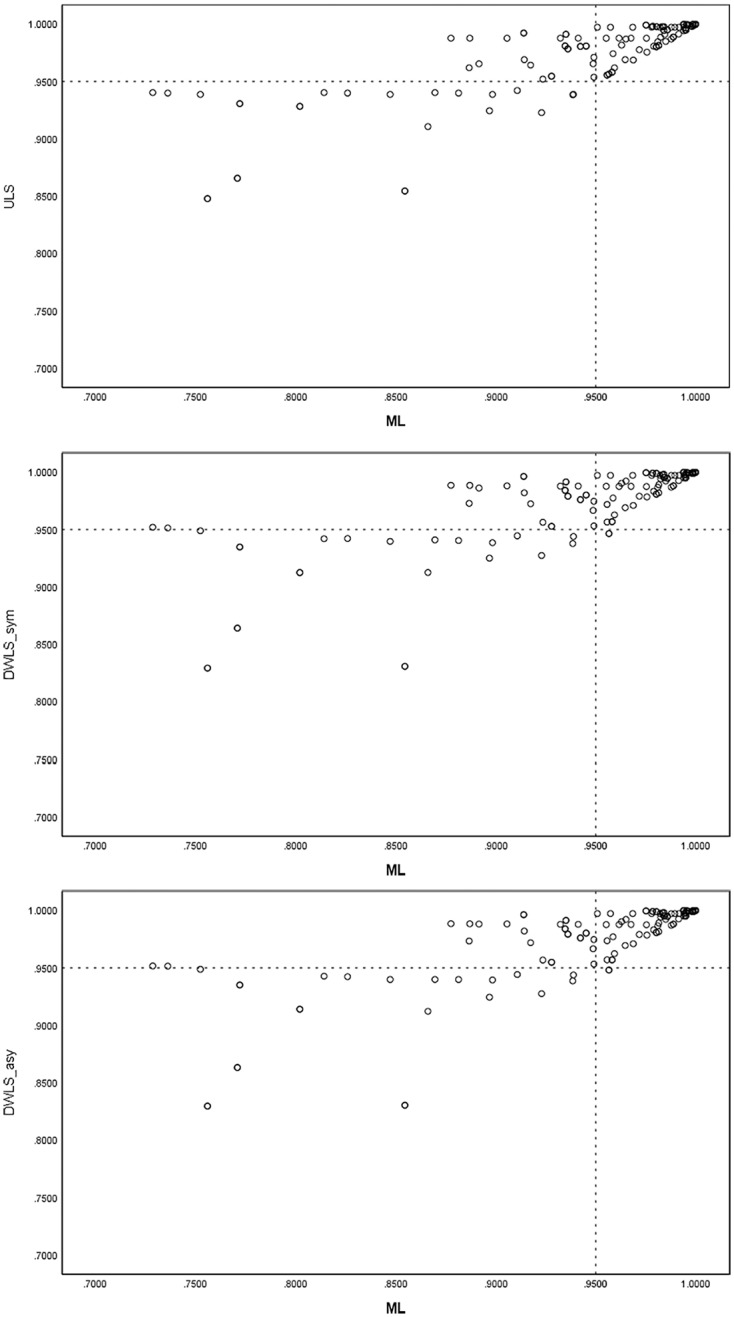
Figure 3.

The relationships between the population SRMRML, SRMRULS, and SRMRDWLS.SRMR = standardized root mean square residual; ML = maximum likelihood; DWLS = diagonally weighted least squares; ULS = unweighted least squares.
The results showed that across all simulated conditions, the population values of SRMR are generally quite robust to the choice of different estimation methods. The R2 of population SRMR between any two of the estimation methods were larger than 99%. As shown in the tables and figures, under all simulated conditions, the differences of population SRMR across estimation methods were ignorable (in the third decimal place), except when the models were severely misspecified (SRMR ≥ .10). However, in general, the difference would not impact the practical interpretation of the model fit results. For example, when fitting a one-factor model to a two-factor data with ρ = .60 (p = 10, λ = .80), the population SRMR were .115 (ML), .115 (ULS), .121 (DWLS with asymmetric thresholds), and .120 (DWLS with asymmetric thresholds), respectively; all population SRMR values suggested that the model fitted the data poorly.
Discussion and Conclusions
The current study examined the effect of estimation methods on the population SEM fit indices (i.e., RMSEA, CFI, and SRMR). Consistent with previous studies (Xia, 2016; Xia & Yang, 2018, 2019), our results showed that given the same type and level of model misspecification, the choice of estimation methods had an important impact on the population values of the RMSEA and CFI. Specifically, for the RMSEA, the population values based on ML can be either greater or smaller than those computed using least squares (i.e., ULS and DWLS). The RMSEAULS was found to be closer to RMSEADWLS than RMSEAML, but noticeable differences can still be observed between RMSEAULS and RMSEADWLS. When using DWLS, the population values of RMSEA also depend on the distribution of the thresholds; RMSEADWLS in models with asymmetric thresholds are consistently larger than RMSEADWLS with symmetric thresholds.
With regard to the CFI, across the simulated conditions considered in the current study, CFIML were generally smaller than those obtained using ULS or DWLS, suggesting that the model fit worse. The difference between CFIULS and CFIDWLS was smaller than the difference between CFIML and CFIULS (or between CFIML and CFIDWLS). Under DWLS, the impact of the distribution of thresholds on population CFI was negligible.
The findings of the current study also expand on conclusions from previous methodological research regarding the influence of estimation methods on the SRMR. The results indicated that given the same type and level of model misspecification, the population values of SRMR are very similar across different estimation methods (i.e., ML, ULS, and DWLS). Why is population SRMR robust to the choice of different estimation methods? As discussed earlier, the population SRMR is computed based on the residual covariance, which is the difference between the population covariance matrix and the model-implied covariance matrix. For any given population covariance matrix, the population SRMR depends on the model-implied covariance matrix. Given the same misspecified model, the model-implied covariance matrix, and thus, the population SRMR is solely determined by the population parameter estimates. Methodological studies have shown that for the same model, the difference in parameter estimates across estimation methods (e.g., ML, ULS, and DWLS) can be trivial, even when the model is misspecified (e.g., Yang-Wallentin, Jöreskog, & Luo, 2010). As a result, the population SRMR is quite insensitive to choices of estimators.
The results of the current research offer implications for empirical studies. Under the situations where the observed data can be treated either as continuous or ordinal (e.g., the number of response categories ≥5), researchers should be aware that the model fit based on RMSEA and CFI can change substantially when different estimation methods are employed. An additional implication of this and previous studies is that the conventional cutoffs for RMSEA and CFI (based on ML) cannot be generalized to situations where categorical estimation methods (e.g., ULS and DWLS) are used. To address this issue, researchers have advocated (a) developing different cutoff values when least squares methods are used (Beauducel & Herzberg, 2006), or (b) computing RMSEAML and CFIML after least squares estimates have been obtained so that cutoff values developed using ML may be used (Savalei, 2017). Our study suggested a third, simpler avenue to overcome this problem: to use the SRMR. We have found in this study that the population SRMR is generally robust to the choice of estimation methods. Therefore, the same population cutoff can be applied when using the SRMR to evaluate model fit, regardless of the choice of estimation method.
This study is not without limitations. First, we only considered three types of model misspecification under factor analysis models. Additional studies should explore the generalizability of the findings to other types of misspecified SEM models. Additionally, we focused on behaviors of the fit indices at the population level. In practice, researchers would only obtain and interpret the sample estimates of the fit indices. Statistical theory enables researchers to construct confidence intervals and tests of close fit for all three population parameters.5 For example, researchers may test the hypothesis , where c is the reference cutoff in the population suggesting close fit.
An alternative, but less rigorous approach, is to directly compare the values on the fit indices with a fixed cutoff value at the sample level. As a reviewer pointed out, even though the population value SRMR is almost the same between ML applied to continuous data and ULS applied to ordinal data, the sample values can be different, because categorical data yield larger sample fluctuations than continuous data. In addition, it is worth noting that for the RMSEA and CFI, when robust corrections are used (e.g., denoted as MLMV, ULSMV in Mplus; Asparouhov & Muthén, 2010; Satorra & Bentler, 1994) to adjust the chi-square test statistics, researchers should pay close attention to the selection of the formula used to compute the sample values. That is, using the current version of most SEM software (e.g., Mplus), the sample RMSEA and CFI based on ML, DWLS, and ULS estimation with robust corrections do not consistently estimate their population values, and they estimate different parameters. To produce relatively unbiased estimates, the unbiased (correct) formula should be used (Brosseau-Liard & Savalei, 2014; Brosseau-Liard, Savalei, & Li, 2012; Gao, Shi, & Maydeu-Olivares, 2019; Li & Bentler, 2006; Savalei, 2018; Xia, 2016). For the SRMR, an unbiased formula has also been developed, which yields more accurate estimates than the RMSEA (Maydeu-Olivares, 2017a; Maydeu-Olivares et al., 2018; Shi, Maydeu-Olivares, & Rosseel, 2019). Future research should investigate the effects of estimation methods on sample SEM fit indices.
Acknowledgments
We acknowledge the Research Computing Center at the University of South Carolina for providing the computing resources that contributed to the results of this article.
It is noted that full-weighted least squares (WLS) is also an available choice for estimating structural equation models for ordinal outcomes. Despite its asymptotic elegance, previous studies have shown that full WLS only perform well when the sample size is very large, and the usage of full WLS is limited in real data analysis (Bandalos, 2014; DiStefano & Morgan, 2014; Flora & Curran, 2004). Therefore, in the current study, we only focus on ULS and DWLS estimators.
When ordinal data are estimated using polychoric correlations, there are two possible sources of misspecifications (Maydeu-Olivares, 2006; Muthén, 1993): distributional and structural. The model may not fit because the assumption of categorized multivariate normality is violated (distributional misspecification) and/or because the structural model (e.g., a one-factor model) is incorrect.
In addition, the SRMR can be estimated very accurately even in small samples (Maydeu-Olivares et al., 2018; Shi, Maydeu-Olivares, et al., 2019).
Recall that the variance of each observed variable is 1.
For the RMSEA, see Browne and Cudeck (1993); for the CFI, see Lai (2019); and for the SRMR, see Maydeu-Olivares (2017a).
Footnotes
Declaration of Conflicting Interests: The author(s) declared no potential conflicts of interest with respect to the research, authorship, and/or publication of this article.
Funding: The author(s) disclosed receipt of the following financial support for the research, authorship, and/or publication of this article: This research is supported in part by the Institute of Education Sciences, U.S. Department of Education, through Grant No. R324A190066, and the National Science Foundation through Grant No. SES-1659936. The opinions expressed are those of the authors. The contents of this paper do not represent the policy of the Department of Education, and you should not assume endorsement by the Federal Government.
ORCID iD: Dexin Shi  https://orcid.org/0000-0002-4120-6756
References
- Asparouhov T., Muthén B. (2010, May). Simple second order chi-square correction scaled chi-square statistics (Technical appendix). Los Angeles, CA: Muthén & Muthén. [Google Scholar]
- Bandalos D. L. (2014). Relative performance of categorical diagonally weighted least squares and robust maximum likelihood estimation. Structural Equation Modeling: A Multidisciplinary Journal, 21, 102-116. [Google Scholar]
- Beauducel A., Herzberg P. Y. (2006). On the performance of maximum likelihood versus means and variance adjusted weighted least squares estimation in CFA. Structural Equation Modeling: A Multidisciplinary Journal, 13, 186-203. [Google Scholar]
- Bentler P. M. (1990). Comparative fit indexes in structural models. Psychological Bulletin, 107, 238-246. [DOI] [PubMed] [Google Scholar]
- Bentler P. M. (1995). EQS 5 [Computer program]. Encino, CA: Multivariate Software. [Google Scholar]
- Box G. E. P. (1979). Some problems of statistics and everyday life. Journal of the American Statistical Association, 74(365), 1-4. [Google Scholar]
- Brosseau-Liard P. E., Savalei V. (2014). Adjusting incremental fit indices for nonnormality. Multivariate Behavioral Research, 49, 460-470. [DOI] [PubMed] [Google Scholar]
- Brosseau-Liard P. E., Savalei V., Li L. (2012). An investigation of the sample performance of two nonnormality corrections for RMSEA. Multivariate Behavioral Research, 47, 904-930. [DOI] [PubMed] [Google Scholar]
- Browne M. W., Cudeck R. (1993). Alternative ways of assessing model fit. In Bollen K. A., Long J. S. (Eds.), Testing structural equation models (pp. 136-162). Newbury Park, CA: Sage. [Google Scholar]
- DiStefano C., Morgan G. B. (2014). A comparison of diagonal weighted least squares robust estimation techniques for ordinal data. Structural Equation Modeling: A Multidisciplinary Journal, 21, 425-438. [Google Scholar]
- Feinian C., Curran P. J., Bollen K. A., Kirby J., Paxton P., Chen F., . . . Paxton P. (2008). An empirical evaluation of the use of fixed cutoff points in RMSEA test statistic in structural equation models. Sociological Methods & Research, 36, 462-494. [DOI] [PMC free article] [PubMed] [Google Scholar]
- Flora D. B., Curran P. J. (2004). An empirical evaluation of alternative methods of estimation for confirmatory factor analysis with ordinal data. Psychological Methods, 9, 466-491. [DOI] [PMC free article] [PubMed] [Google Scholar]
- Forero C. G., Maydeu-Olivares A., Gallardo-Pujol D. (2009). Factor analysis with ordinal indicators: A Monte Carlo study comparing DWLS and ULS estimation. Structural Equation Modeling: A Multidisciplinary Journal, 16, 625-641. [Google Scholar]
- Gao C., Shi D., Maydeu-Olivares A. (2019). Estimating the maximum likelihood root mean square error of approximation (RMSEA) with non-normal data: A Monte-Carlo study. Structural Equation Modeling: A Multidisciplinary Journal, 27(2), 192-201. doi: 10.1080/10705511.2019.1637741 [DOI] [Google Scholar]
- Hu L., Bentler P. M. (1999). Cutoff criteria for fit indexes in covariance structure analysis: Conventional criteria versus new alternatives. Structural Equation Modeling: A Multidisciplinary Journal, 6, 1-55. [Google Scholar]
- Jöreskog K. G. (1969). A general approach to confirmatory maximum likelihood factor analysis. Psychometrika, 34, 183-202. [Google Scholar]
- Jöreskog K. G., Sörbom D. (1988). LISREL 7. A guide to the program and applications (2nd ed.). Chicago, IL: International Education Services. [Google Scholar]
- Kenny D. A., Kaniskan B., McCoach D. B. (2015). The performance of RMSEA in models with small degrees of freedom. Sociological Methods & Research, 44, 486-507. [Google Scholar]
- Lai K., (2019). A Simple Analytic Confidence Interval for CFI Given Non-normal Data. Structural Equation Modeling: A Multidisciplinary Journal, 26(5), 757-777. [Google Scholar]
- Li L., Bentler P. M. (2006). Robust statistical tests for evaluating the hypothesis of close fit of misspecified mean and covariance structural models (UCLA Statistics Preprint No. 506). Los Angeles: University of California, Los Angeles. [Google Scholar]
- MacCallum R. C. (2003). Working with imperfect models. Multivariate Behavioral Research, 38, 113-139. [DOI] [PubMed] [Google Scholar]
- MacCallum R. C., Browne M. W., Sugawara H. M. (1996). Power analysis and determination of sample size for covariance structure modeling. Psychological Methods, 1, 130-149. [Google Scholar]
- Maydeu-Olivares A. (2006). Limited information estimation and testing of discretized multivariate normal structural models. Psychometrika, 71, 57-77. [Google Scholar]
- Maydeu-Olivares A. (2017. a). Assessing the size of model misfit in structural equation models. Psychometrika, 82, 533-558. [DOI] [PubMed] [Google Scholar]
- Maydeu-Olivares A. (2017. b). Maximum likelihood estimation of structural equation models for continuous data: Standard errors and goodness of fit. Structural Equation Modeling: A Multidisciplinary Journal, 24, 383-394. [Google Scholar]
- Maydeu-Olivares A., Cai L., Hernández A. (2011). Comparing the fit of item response theory and factor analysis models. Structural Equation Modeling: A Multidisciplinary Journal, 18, 333-356. [Google Scholar]
- Maydeu-Olivares A., Shi D., Rosseel Y. (2018). Assessing fit in structural equation models: A Monte-Carlo evaluation of RMSEA versus SRMR confidence intervals and tests of close fit. Structural Equation Modeling: A Multidisciplinary Journal, 25, 389-402. [Google Scholar]
- McNeish D., An J., Hancock G. R. (2018). The thorny relation between measurement quality and fit index cutoffs in latent variable models. Journal of Personality Assessment, 100, 43-52. [DOI] [PubMed] [Google Scholar]
- Moshagen M. (2012). The model size effect in SEM: Inflated goodness-of-fit statistics are due to the size of the covariance matrix. Structural Equation Modeling: A Multidisciplinary Journal, 19, 86-98. [Google Scholar]
- Muthén B. (1993). Goodness of fit with categorical and other nonnormal variables. In Bollen K. A., Long J. S. (Eds.), Testing structural equation models (pp. 205-234). Newbury Park, CA: Sage. [Google Scholar]
- Muthén B. O., du Toit S. H. C., Spisic D. (1997, November 18). Robust inference using weighted least squares and quadratic estimating equations in latent variable modeling with categorical and continuous outcomes. Retrieved from https://www.statmodel.com/download/Article_075.pdf
- R Core Team. (2019). R: A language and environment for statistical computing. Vienna, Austria: R Foundation for Statistical Computing. [Google Scholar]
- Rhemtulla M., Brosseau-Liard P. É., Savalei V. (2012). When can categorical variables be treated as continuous? A comparison of robust continuous and categorical SEM estimation methods under suboptimal conditions. Psychological Methods, 17, 354-373. [DOI] [PubMed] [Google Scholar]
- Rosseel Y. (2012). lavaan: An R package for structural equation modeling. Journal of Statistical Software, 48(2), 1-36. [Google Scholar]
- Saris W. E., Satorra A., van der Veld W. M. (2009). Testing structural equation models or detection of misspecifications? Structural Equation Modeling: A Multidisciplinary Journal, 16, 561-582. [Google Scholar]
- Satorra A. (1990). Robustness issues in structural equation modeling: A review of recent developments. Quality and Quantity, 24, 367-386. [Google Scholar]
- Satorra A., Bentler P. M. (1994). Corrections to test statistics and standard errors in covariance structure analysis. In Von Eye A., Clogg C. C. (Eds.), Latent variable analysis. Applications for developmental research (pp. 399-419). Thousand Oaks, CA: Sage. [Google Scholar]
- Savalei V. (2012). The relationship between root mean square error of approximation and model misspecification in confirmatory factor analysis models. Educational and Psychological Measurement, 72, 910-932. [Google Scholar]
- Savalei V. (2017). Reconstructing fit indices in SEM with categorical data: Borrowing insights from nonnormal data. Paper presented at the Annual Meeting of the Society of Multivariate Experimental Psychology, Minneapolis, MN. [Google Scholar]
- Savalei V. (2018). On the computation of the RMSEA and CFI from the mean-and-variance corrected test statistic with nonnormal data in SEM. Multivariate Behavioral Research, 53, 419-429. [DOI] [PubMed] [Google Scholar]
- Savalei V., Rhemtulla M. (2013). The performance of robust test statistics with categorical data. British Journal of Mathematical and Statistical Psychology, 66, 201-223. [DOI] [PubMed] [Google Scholar]
- Shi D., DiStefano C., McDaniel H. L., Jiang Z. (2018). Examining chi-square test statistics under conditions of large model size and ordinal data. Structural Equation Modeling: A Multidisciplinary Journal, 25, 924-945. [Google Scholar]
- Shi D., Lee T., Maydeu-Olivares A. (2019). Understanding the model size effect on SEM fit indices. Educational and Psychological Measurement, 79, 310-334. [DOI] [PMC free article] [PubMed] [Google Scholar]
- Shi D., Lee T., Terry R. A. (2015). Abstract: Revisiting the model size effect in structural equation modeling (SEM). Multivariate Behavioral Research, 50, 142-142. [DOI] [PubMed] [Google Scholar]
- Shi D., Lee T., Terry R. A. (2018). Revisiting the model size effect in structural equation modeling. Structural Equation Modeling: A Multidisciplinary Journal, 25, 21-40. [Google Scholar]
- Shi D., Maydeu-Olivares A., DiStefano C. (2018). The relationship between the standardized root mean square residual and model misspecification in factor analysis models. Multivariate Behavioral Research, 53, 676-694. [DOI] [PubMed] [Google Scholar]
- Shi D., Maydeu-Olivares A., Rosseel Y. (2019). Assessing fit in ordinal factor analysis models: SRMR vs. RMSEA. Structural Equation Modeling: A Multidisciplinary Journal, 27(1), 1-15. doi: 10.1080/10705511.2019.1611434 [DOI] [Google Scholar]
- Steiger J. H. (1989). EzPATH: A supplementary module for SYSTAT and SYGRAPH. Evanston, IL: Systat. [Google Scholar]
- Steiger J. H. (1990). Structural model evaluation and modification: An interval estimation approach. Multivariate Behavioral Research, 25, 173-180. [DOI] [PubMed] [Google Scholar]
- Steiger J., Lind J. C. (1980). Statistically based tests for the number of common factors. Paper presented at the annual Spring Meeting of the Psychometric Society, Iowa City. [Google Scholar]
- Xia Y. (2016). Investigating the chi-square-based model-fit indexes for WLSMV and ULSMV estimators (Unpublished doctoral dissertation). Florida State University, Tallahassee, FL. [Google Scholar]
- Xia Y., Yang Y. (2018). The influence of number of categories and threshold values on fit indices in structural equation modeling with ordered categorical data. Multivariate Behavioral Research, 53, 731-755. [DOI] [PubMed] [Google Scholar]
- Xia Y., Yang Y. (2019). RMSEA, CFI, and TLI in structural equation modeling with ordered categorical data: The story they tell depends on the estimation methods. Behavior Research Methods, 51, 409-428. [DOI] [PubMed] [Google Scholar]
- Yang-Wallentin F., Jöreskog K. G., Luo H. (2010). Confirmatory factor analysis of ordinal variables with misspecified models. Structural Equation Modeling, 17, 392-423. [Google Scholar]