The ONIOM/PMM Model for Effective Yet Accurate Simulation of Optical and Chiroptical Spectra in Solution: Camphorquinone in Methanol as a Case Study

Abstract

This paper deals with the development and first validation of a composite approach for the simulation of chiroptical spectra in solution aimed to strongly reduce the number of full QM computations without any significant accuracy loss. The approach starts from the quantum mechanical computation of reference spectra including vibrational averaging effects and taking average solvent effects into account by means of the polarizable continuum model. Next, the snapshots of classical molecular dynamics computations are clusterized and one reference configuration from each cluster is used to compute a reference spectrum. Local fluctuation effects within each cluster are then taken into account by means of the perturbed matrix model. The performance of the proposed approach is tested on the challenging case of the optical and chiroptical spectra of camphorquinone in methanol solution. Although further validations are surely needed, the results of this first study are quite promising also taking into account that agreement with experimental data is reached by just a couple of full quantum mechanical geometry optimizations and frequency computations.

1. Introduction

Characterization of chiral compounds is a central issue in several fields, such as catalysis, materials, and life science.¹⁻³ Chiroptical spectroscopies represent the techniques of choice to investigate in a noninvasive way the physical–chemical properties of chiral systems, especially in condensed phases. Among these spectroscopies, electronic circular dichroism (ECD), that is the differential absorption of left- and right-handed circularly polarized light, has played a prominent role for the study of the absolute stereochemistry and conformation of chiral molecules.⁴ While absorption spectra are capable of characterizing ground electronic states and their environment, emission spectra and their chiral counterpart (circularly polarized luminescence, CPL) allow investigation of the properties of the excited electronic state from which the emission occurs. Therefore, combination of several spectroscopic techniques is essential to achieve a comprehensive and unbiased characterization of the molecular systems. However, experimental spectra can seldom be interpreted by means of classical or phenomenological models.⁵ Thanks to the continuous advances of hardware and software, the accuracy of computational simulations for medium-size semirigid systems in the gas phase rivals that of the corresponding experimental results thus providing an invaluable aid for assignment and interpretation of spectroscopic outcomes increasingly used also by nonspecialists.^6,7

Nevertheless, the study of large flexible systems faces a number of difficulties (even within the Born–Oppenheimer approximation) ranging from the very unfavorable scaling of those methods with the number of active electrons to the proper description of flat potential energy surfaces (PESs) with not well-defined stationary points. In condensed phases, the number of degrees of freedom to be taken into account increases dramatically, so that not-trivial aspects of statistical mechanics come into play, the situation being particularly tricky for noninnocent solvents, where solute–solvent and solvent–solvent interactions are of comparable strength.⁸ Despite the advances of the so-called ab initio molecular dynamics pioneered by Car and Parrinello,⁹ classical molecular mechanics (MM) remains the computational tool of choice for this purpose, with Monte Carlo (MC) and Molecular Dynamics (MD) simulations being the two main sampling techniques employed.¹⁰ Unfortunately, the range of applicability of conventional classical methods is quite limited in the context of molecular spectroscopy because they cannot address all the processes and phenomena explicitly related to the electronic degrees of freedom. At least for localized phenomena, the most viable strategy is thus offered by the multiscale or multiresolution methods pioneered by Karplus, Levitt, and Warshel¹¹ (awarded the Nobel Prize in 2013), which rely on the integration of a number of computational protocols and algorithms.^12,13 In multiresolution methods the focus is kept on the target system (treated at the QM level), while the environment can be progressively blurred from an atomistic MM treatment up to a mean field description.⁸ Over the last few decades, these methods have met remarkable success also thanks to remarkable improvements in hardware and software.¹⁴⁻¹⁷ However, a number of developments are still needed to extend the range of application for computational and spectroscopic simulations. In this connection, chiroptical spectrocopies play an increasing role, but involve also significant technical problems related to the coupling of small intensity with high sensitivity to environmental effects.¹⁸⁻²⁸

Along these lines, the aim of the present contribution is to propose and validate a reliable yet effective computational strategy for the modeling of vibrationally resolved absorption and emission spectra of chiral molecules in solution by combining different theoretical–computational procedures. The final spectra stem from successive refinements, that is from an additive multistep procedure achieved by adding the outcomes of methods of decreasing accuracy when moving from the chromophore to its cybotactic region, to bulk solvent. In detail, accurate theoretical/computational models were employed to evaluate the quantum properties of the chromophore in solution for some relevant solute–solvent configurations including vibrational modulation effects produced by small-amplitude motions, but then an approximated yet robust scheme was applied to model the effects of the thermal fluctuations of the embedding environment on the quantum properties. In particular, we applied the recently developed integrated variational/perturbative approach (ONIOM/EE-PMM)²⁹ to model both absorption and emission spectra of Camphorquinone (CQ) dye in methanol.

Our ONIOM/EE-PMM procedure falls into the category of Quantum Mechanics/Molecular Mechanics (QM/MM) approaches, for which a suitable part of the system is described at the QM level, while the remainder is described classically. The starting point of the procedure is the classical simulation of the complete system (through Molecular Dynamics, MD, or Monte Carlo, MC, simulations). The effectiveness of the method relies in the application of a variational approach (i.e., ONIOM calculation with the Electronic Embedding scheme, EE^12,30,31) only for “reference” snapshots of the simulation that might be representative of each subtrajectory found through a cluster analysis of the complete classical sampling. Next, an effective perturbative approach (i.e., Perturbed Matrix Method, PMM³²⁻³⁴) is applied to treat the local fluctuations within each cluster. When compared with the standard procedures, from one side, the approach allows us to cut down the computational costs due to the extensive trajectory subsampling utilized for successive QM computations; from the other, it allows us to prevent inaccuracies due to application of a perturbative approach for configurations strongly different from the reference one. Although combination of classical MD with clustering and QM computations has been extensively employed^35,36 also in connection with chiroptical spectroscopies,³⁷ the result of the trajectory partitioning depends not only on the computational procedure utilized (e.g., the clustering procedures) but also on the observable determining the partitioning of the system. A sensible choice might be based on the conformational fluctuations of the solute (QM) layer of the system. For instance, for a similar application, we recently³⁸ applied a density-based spatial clustering method to the bidimensional subspace spanned by the first two principal components of the solute atomic fluctuations. Likewise, when a rigid or semirigid solute is taken into account, the complete trajectory can be thought as a single extensive conformational basin thus applying the procedure by means of a single QM calculation. Nevertheless, even for such a simple case, the selection of the reference structure on which the QM calculation is performed represents an issue of major relevance. This choice, in fact, affects (even if not dramatically) the final results. In the present contribution we studied a semirigid solute (CQ, vide supra) that allowed us to exploit the very cheap model based on a “single-reference” structure, whose selection is thoroughly addressed in the paper with the aim of providing a general and robust solution to the problem.

For the present study, we applied the aforementioned procedure to reproduce the one photon absorption (OPA) and emission (OPE) spectra of the chromophore in solution including ECD and CPL spectra, thus reporting for the first time (to the best of our knowledge) an application of the PMM to chiroptical spectra. Noticeably, the task is of remarkable complexity given the tiny values and sensitivity of the observables characterizing the inherent phenomena. Here, vibrational contributions are often critical and need to be properly accounted for to modulate the shape and improve the overall agreement with experimental results.^6,39 CQ was chosen because it is a small organic diketone widely investigated for its spectroscopic properties.⁴⁰⁻⁴³ In particular, CQ shows a well isolated first absorption band and emits by both fluorescence and phosphorescence (assessment of the latter is beyond the scope of the present contribution) depending on the environmental conditions,^40,41 with both kinds of spectra being clearly modulated by vibrational contributions. These characteristics make CQ an appealing model system to develop and test new computational protocols.^6,44 We pushed the modelization beyond the characterization of the pure electronic spectra by combining the ONIOM/EE-PMM results with the outcomes of fully quantum mechanical procedures for simulating vibronic effects for both optical and chiroptical spectra.

In summary, we propose and validate an effective procedure for the simulation of optical and chiroptical spectra in solution, developed to optimize the accuracy of the description while limiting the computational effort. To this end, we applied a multiscale procedure based on tuning the level of theory employed to investigate each property involved in the spectroscopic processes according to its estimated impact on the final results. The proposed procedure can be summarized as follows:

• 1.Equilibrium geometries of both the ground and first excited states of the chromophore were generated by means of QM approaches rooted into the density functional theory (DFT) and its time-dependent extension (TD-DFT).
• 2.Force-field (FF) parameters (at least solute atomic charges) were derived for the successive classical simulations possibly including average solvent effects by the polarizable continuum model (PCM).
• 3.Starting from the solvated equilibrium geometries of the chromophore (for each relevant electronic state), classical simulations were performed to provide the statistical ensembles accounting for the solute–solvent interactions.
• 4.Trajectory partitioning and analysis were applied to identify the solute–solvent configurations most representative of the solvent effects.
• 5.Quantum mechanical calculations taking into account the effects of the embedding environment by means of variational approaches (i.e., ONIOM/EE procedure) were performed for the representative snapshots.
• 6.For all the remaining snapshots of the simulation the perturbative approach (i.e., PMM) was applied to model the effects on the chromophore quantum properties of the fluctuations of the embedding environment with respect to the representative snapshots.
• 7.The absorption/emission electronic spectra and their chiroptical counterparts were computed by means of the properties obtained from points 5 and 6.
• 8.Finally, vibronic effects in the electronic spectra were added by using QM models based on the Franck–Condon principle.

The same procedure is also sketched in Figure 1 where each of the theoretical/computational frameworks applied is ranked according to a (qualitative) scale of accuracy. For the present case, the structural rigidity of the chromophore allowed us to introduce approximations that simplified the application of the overall procedure. Namely, (i) we performed the classical simulations of the system by constraining the solute in its equilibrium geometry (point 2 of the list above) and (ii) we considered the vibrational modulation of the electronic spectra as a constant term to be simply added to the electronic spectra (point 8 of the list above). In particular the latter approximation will become too rough whenever semiclassical internal coordinates of the chromophore were to be taken into account. Although general and effective procedures have been developed to deal with those more complex situations,²⁹ in the present contribution we will be concerned only with rigid solutes.

Figure 1.

Outline of our computational strategy: graphical representation of the main theoretical frameworks employed (upper panel) and workflow of the procedure (lower panel).

2. Methods

2.1. Molecular Dynamics Simulation and Analysis

The simulations of both the ground and first excited electronic state of CQ in methanol were carried out with the Gromacs software package.⁴⁵ During each production run the chromophore was constrained in the minimum energy structure of the relevant electronic state, which is quite rigid due to the presence of the intramolecular methylene bridge and the two carbonyl groups. The CQ structure can be seen in Figure 2, Panel A, where a sphere extracted from a representative frame of the CQ in methanol ground state simulation is reported. The solute atomic charges were computed in vacuum at the equilibrium structure of either the ground or first excited electronic state by means of the RESP model.⁴⁶ The nonbonded parameters were obtained from the GROMOS96 54a7 force field.⁴⁷ The vacuum optimization and the atomic charges calculations were performed by using density functional theory (DFT)⁴⁸ with the hybrid B3LYP functional^49,50 in conjunction with cc-pVDZ⁵¹ basis set using the Gaussian16 package⁵² as already done in similar investigations.⁵⁵ For the CQ ground state we computed also the equilibrium structure and atomic charges by mimicking solvent effects by means of the polarizable continuum model (PCM).^54,55 Negligible differences were found when comparing the results of the two computations, well within the expected accuracy of the level of theory employed (see Figure S2 in SI). Therefore, we utilized the vacuum geometries and charges to maximize the transferability of the topology. However, despite the rigidity of the molecule, we preferred to utilize the PCM equilibrium geometries for the ONIOM-EE calculations employed for the final spectra as a further refinement. Indeed, the RMSD among the vacuum and PCM energy minimum for the ground state is 0.009 Å, while the corresponding value for the first electronic excited state is 0.006 Å. The AMBER model was utilized for the methanol topology.⁵⁶ The simulations were carried out in the isothermal–isochoric ensemble (NVT) with periodic boundary conditions, using an integration step of 2 fs. The temperature was kept constant (300 K) by the velocity-rescaling⁵⁷ temperature coupling. The bonds were constrained using the LINCS algorith.⁵⁸ The particle mesh Ewald method⁵⁹ was used to compute long-range interactions with grid search and cutoff radii of 1.1 nm. A cubic simulation box was utilized, calibrating the density to obtain in the NVT MD simulations a pressure identical, within the noise, to the one provided by a corresponding reference MD simulation of the pure solvent. Such reference simulation of pure methanol was carried out in the NVT ensemble setting T = 300 K and imposing a box density equal to the experimental density of the corresponding pure methanol at the standard p,T conditions (24.58 mol per L⁶⁰). Both the production runs were of 10 ns.

Figure 2.

(Panel A) Sphere extracted from a representative frame of the CQ in methanol (ground state) MD simulation where the chromophore engages in HB with two methanol molecules through the outward VSs (the molecules involved in the interaction are highlighted). (Panels B and C) Radial and angular distribution functions for each VS (refer to panels D and A for the VS’s code color). (Panel D) F function for each VS.

The ground state of the system was also simulated by modeling the charge separation on the oxygen atoms (that is, the lone pairs) by means of virtual interaction sites. Virtual sites (VS) were located at the position corresponding to the centroids of localized molecular orbitals for the sp2 oxygen atom using the Boys localization procedure, as reported in ref (61). Each VS-oxygen distance was constrained during the simulation. A partial charge was assigned to each VS in order to reproduce the classical dipole of the molecule. From the ground state calculation of the atomic charges, we obtained almost identical values for the two oxygen atoms, that we averaged to −0.390. To ensure the same degree of symmetry, we imposed the charges of the inward and outward VSs to have the same values (−0.105 and −0.285, respectively) for both oxygen atoms. Inclusion of VSs was meant to account for the directionality of hydrogen bonding (HB). In fact, we analyzed the probability of HB between the two carbonyl groups of CQ and the hydroxyl group of methanol using a function (known as F function)^29,62 which exploits the fulfillment of geometrical criteria to compute the probability of HB per atom for each MD time frame. The function is equal to 1 if the deviations from reference values of both the HB donor–acceptor distance and the angle they form with the oxygen in methanol are smaller than a threshold value, while it decreases exponentially for increasing deviations. It is interesting to note that from the calculation of the first excited state atomic charges we obtained an average value of −0.385 for the two oxygen atoms. For comparison, the corresponding values obtained by means of the CM5⁶³ model are −0.26 and −0.25 for the ground and excited state, respectively (vide infra). More detailed comparisons of different atomic charge models can be found in the SI.

2.2. Electronic Spectra Calculations

2.2.1. ONIOM Calculations

We applied the ONIOM/EE procedure to compute OPA and ECD spectra. We considered the solute as the model system (that is, the system subpart to be treated at the QM level according to the ONIOM paradigm) while the methanol atoms were treated as embedding charges within the electronic embedding (EE) scheme. Since the procedure has been extensively reviewed,^12,31,64,65 we only summarize some basic aspects. The interaction with the embedding charges is included into the QM Hamiltonian as

1

where Ĥ^QM represents the QM Hamiltonian in the absence of the environment and the N, J, and i indexes refer to the environment atoms, the atoms of the model system, and the electrons, respectively. q are the embedded charges, Z are the nuclear charges of the atoms of the model system, and r is the distance between each of the environment atoms and the atoms or electrons in the QM region (s is a scaling factor used to avoid overpolarization of the wave function due to large charges close to the QM region; it is zero for charges less than three bonds away from the QM region and one for the remaining charges). The procedure was applied by extracting sequentially 200 snapshots from the ground state CQ in the methanol trajectory to be utilized for the time dependent (TD) DFT⁶⁶ computations at the B3LYP/6-311G(d)⁶⁷ level. The resulting excitation energies and oscillator strengths of the ground to first excited state transition were extracted from each calculation. For the pure electronic OPA spectrum, the half-width at half-maximum (HWHM) of the Gaussian function used to convolute the transitions was set to 900 cm^–1. For the pure electronic absorption spectrum, we utilized the CQ geometry optimized in vacuum, whereas we employed the CQ energy minimum in PCM to compute the final vibronic spectra (see subsections below).

2.2.2. Hybrid ONIOM/EE-PMM Calculations

Theoretical Framework. We applied the ONIOM/EE-PMM procedure that we proposed in our recent paper.²⁹ In detail, for the representative frame of the simulation a variational procedure (ONIOM/EE) is employed to solve the QM Hamiltonian incorporating the partial charges of the embedding environment³¹(Ĥ^EE). For all the remaining frames of the simulation, the perturbing effects exerted by the environment are provided by diagonalizing the perturbed Hamiltonian matrix H̃ built in the basis set of the eigenstates obtained from the previous calculation (Ψ_l^EE). Accordingly, a perturbation operator is defined to model the fluctuations of the electrostatic potential exerted by the atomistic environment for each MD frame with respect to the one accounted for by the ONIOM/EE calculation, namely

2

where

3

and

4

For each frame of the simulation, the operator ΔV̂ models the variation between the perturbing effects exerted by the environment in that frame and the reference. For the present application, the latest development of the PMM procedure is by expanding the perturbing electrostatic potential within the atomic region around each atomic center (atom-based expansion).⁶⁸ Interested readers can find details of the procedure in refs (29, 30, 68) while details of the computations are reported in the following subsections.

Choice of the Reference Structure. For the present contribution we developed a general and unbiased procedure to select the reference frame to be employed for the (ONIOM/EE) QM calculation from each preidentified cluster within the simulation. Its basic rationale consists in employing an average configuration of the molecular environment. This is achieved by extracting a number N of snapshots from the trajectory, assembling them into a collective configuration, and assigning to each environmental atom 1/N of the actual atomic charge. The N snapshots are extracted sequentially from the trajectory, setting the step for the extraction according to N and the total length of the trajectory. A snapshot can be employed only if none of its atoms overlap any atom of the collective snapshot; otherwise, it is discarded and the following one is evaluated. From each of the selected snapshots, before creating the collective frame, we extracted a sphere centered around the solute in order to limit the number of atoms employed for the electronic embedding calculation. We selected the size of the sphere by computing the electric field acting on the solute center of mass as due to the atomic embedding environment for a snapshot extracted randomly from the trajectory. In fact, we noticed that beyond 30 Å from the solute center of mass, the electric field does not significantly change its intensity (data not shown). Hence we utilized a 30 Å radius sphere, in line with the typical size employed, for instance, when MD with nonperiodic boundary conditions are performed or for similar QM/MM applications.^69,70 The next point to be analyzed was the number of snapshots to be collected together. We decided to utilize 30 snapshots as resulting from balancing the total number of atoms employed for the embedding calculation, the occurrence of atomic clashes (the greater the number of snapshots is, the more likely the atoms will overlap), and the convergence of the results. To derive the final setup we performed a number of calculations on different collective snapshots. The results of the test are summarized in Table 1 where the transition energies and transition electric dipole moments referring to the ground to first excited state transition are reported. In the same table we also report, for the sake of comparison, the corresponding results obtained by (i) collecting 20 configurations sequentially extracted from the trajectory when the complete box is utilized instead of the cut sphere (full box configuration) and (ii) following the procedure we previously employed (that is, extracting the frame characterized by the electric field components closest to the average values, mean electric field configuration).

Table 1. Outcomes of the Electronic Embedding Calculations for the Reference Configuration Selection.

No. of configurations	Transition Energy	Transition Dipole Strength	No. of atoms
30 Å sphere
1	2.4800 eV (499.94 nm)	0.0025	1679
5	2.4716 eV (501.64 nm)	0.0027	8320
10	2.4784 eV (500.25 nm)	0.0028	16618
15	2.4780 eV (500.34 nm)	0.0028	24911
20	2.4778 eV (500.39 nm)	0.0028	33226
25	2.4766 eV (500.61 nm)	0.0029	41398
30	2.4773 eV (500.48 nm)	0.0029	49843
35	2.4833 eV (499.27 nm)	0.0029	58065
40	2.4794 eV (500.06 nm)	0.0029	66249
45	2.4771 eV (500.52 nm)	0.0026	74546
50	2.4812 eV (499.70 nm)	0.0029	82896
55	2.4768 eV (500.57 nm)	0.0029	91228
60	2.4770 eV (500.54 nm)	0.0029	99591
65	2.4757 eV (500.79 nm)	0.0028	107783
70	2.4795 eV (500.04 nm)	0.0029	115966
40 Å sphere
1	2.4805 eV (499.83 nm)	0.0025	3933
5	2.4717 eV (501.62 nm)	0.0027	19599
10	2.4785 eV (500.23 nm)	0.0028	39204
15	2.4780 eV (500.34 nm)	0.0028	58749
20	2.4816 eV (499.62 nm)	0.0030	78227
25	2.4766 eV (500.62 nm)	0.0029	97836
30	2.4774 eV (500.47 nm)	0.0029	117470
35	2.4833 eV (499.28 nm)	0.0029	137038
Full box configuration
20	2.4799 eV (499.96 nm)	0.0029	137180
Mean electric field configuration
1	2.4850 eV (498.94 nm)	0.0029	6859

Spectra calculations. In order to apply the perturbative approach, the first 11 electronic states and the complete matrix of the corresponding dipole moments for the reference configuration were computed using TD DFT theory exploiting the ONIOM/EE model. For each electronic state, the corresponding atomic charges were also computed according to the RESP methodology by employing the same level of theory. In the Results section the pure electronic spectra (as resulting from the ground to first perturbed excited state transition) obtained from different reference configurations are first reported. These configurations differ in the solvent molecular arrangement while the solute geometry is the same, corresponding to the energy minimum in vacuum. We utilized an HWHM of 900 cm^–1 for the Gaussian function used to convolute the transitions. The same TD-DFT calculations mentioned above were carried out on the collective configuration for the PCM equilibrium geometry of CQ to get a refined set of results to be used in conjunction with the vibronic results (vide infra). The computations were carried out with the Gaussian16 package.⁵²

2.3. Vibronic Contributions

PCM Vibronic Calculations. Vibrational modulation (vibronic) effects in electronic spectra were accounted for using models based on the Franck–Condon principle. For a more detailed description of the framework, interested readers are addressed to refs (39, 71, and 72). In this work we relied on the so-called time-independent (TI) approach, in which the band-shape can be obtained as a sum of the individual transitions between the vibrational states of the initial and final electronic states. A general formulation to compute spectrum intensity can be expressed as

5

where * represents the conjugate of d_if^B and δ is the Dirac function.³⁹

From eq 5 the intensity for a specific spectroscopy can be obtained by replacing the α, β, γ, d_if^A, and d_if with the proper values reported in Table 2.

Table 2. Equivalence Table to Compute the Spectrum Intensity for the Spectroscopies of Interest from Eq 5.

Observable	α	β	γ	difA	difB
OPA	10NAπ/3ε0 ln(10)ℏc	1	m	μmn	μmn
OPE	2NA/3ε0c3	4	n	μmn	μmn
ECD	40NAπ/3ε0 ln(10)ℏc2	1	m	μmn	mmn
CPL	8NA/3ε0c4	4	n	μmn	mmn

The computation of transition integrals requires the vibrational frequencies and the normal modes of each electronic state involved, which are connected by means of the Duschinsky transformation,⁷³ an approximation that has been shown to be reliable for semirigid systems.^39,71,72 One critical aspect is that the electronic excitation process can lead to geometry variations resulting in differences of two PESs and shifts of the two minima. Two different strategies can be adopted to account for these effects: either to compute each PES at its own energy minimum in order to optimize the overall description (adiabatic models) or to compute the PES about the vertical transition to better reproduce the most prominent transitions (vertical models). For both descriptions, force constants can be evaluated for each electronic state improving the accuracy (adiabatic Hessian, AH, and vertical Hessian, VH) or the computational cost can be reduced employing identical curvatures for both electronic states, so that only the less demanding Hessian, namely that of the ground state, is explicitly computed (adiabatic shift, AS, and vertical gradient, VG).

Finally, the dependence of the transition moments on the nuclear position is accounted for through expansion of the transition moments as Taylor series around one equilibrium geometry taken as a reference. The zeroth-order and first-order terms represent respectively the Franck–Condon (FC) and Herzberg–Teller (HT) contributions. In this paper, the FCHT acronym will be used to indicate the inclusion of both terms in the calculations.

We simulated vibronic spectra starting from the structure and force constants computed taking into account solvent effects by PCM. Absorption spectra have been computed employing VG|FC, AH|FC, and AH|FCHT models, whereas only adiabatic models (AH|FC and AH|FCHT) have been employed in the case of emission spectra. The default Gaussian parameters of the class-based integral prescreening scheme have been employed (C₁^max = 20, C₂= 13, N_I^max = 10⁹), achieving progression above 90% in every calculation. Gaussian distribution functions with HWHM of 450 cm^–1 have been used as broadening functions.

Ensemble Vibronic Calculations. The vibrationally resolved spectra accounting for the solvent effects as provided by the MD trajectory were computed starting from the corresponding vibronic spectra obtained from single calculations performed by means of PCM. A value of 400 cm^–1 was used as HWHM of the Gaussian distribution functions employed for broadening. We utilized a smaller value than the one employed in conjunction with the PCM since, for this case, either the ONIOM/EE or ONIOM/EE-PMM procedures fully provided the effects due to environment fluctuations. At the FC level, the final spectra were obtained by scaling the vibronic contribution (as obtained from the PCM calculation) by the corresponding perturbed transition energy and oscillator/rotatory strength for each MD snapshot (the last, corresponding to either the trajectory subsampling or the complete MD trajectory according to employing the ONIOM/EE or ONION/EE-PMM procedure, respectively). Specifically, each vibronic spectrum was shifted by the energy difference between the transition energy in PCM and the perturbed one, while the normalized PCM intensity was multiplied in the perturbed energy and corresponding property. When applying the ONIOM/EE-PMM procedure for chiroptical spectroscopy, a further approximation was introduced. In fact, we considered the embedding environment as perturbing only the electric properties of CQ. That is, we employed our procedure to obtain a “trajectory” of perturbed electric transition dipole moments while we considered the magnetic dipole moment as unaffected by the environment fluctuation effects. Thus, for each MD snapshot we computed the rotatory strength by means of the corresponding perturbed electric transition dipole moment and the magnetic transition dipole computed on the reference configuration. At variance, the ONIOM/EE procedure provides for each QM calculation both the electric and magnetic transition dipole moments to get the corresponding rotatory strength. Therefore, comparing the distributions of the angles between the transition dipole moments and the values of rotatory strength obtained with both the ONIOM/EE and the ONIOM/EE-PMM procedures, we were able to evaluate and support the validity of our approximation in the system under investigation (see section 3 in the SI).

In order to go beyond the FC level, the derivatives of the transition dipole moments are needed, which would require, in turn, computation of the derivatives of the perturbed transition dipole moments for each MD snapshot. Since this model would become too computationally demanding, further approximations are needed. To this end we assumed that the difference between the full FCHT spectrum and its FC counterpart for the reference configuration is modulated by solvent fluctuations by a constant amount proportional to that explicitly computed for the FC part as described above. Since reasonable choices of the scaling factor led to comparable results, we decided to use the same value of 1/2 for all kinds of spectra.

3. Results

3.1. Ground and First Excited State Molecular Dynamics

As mentioned above, the ground state simulation of CQ was performed both by locating point charges on the solute atomic positions and by employing VSs to account for the presence of the lone pairs on the solute oxygen atoms. For each HB acceptor in CQ (i.e., either the oxygen atoms or the VSs, according to the trajectory analyzed), for each MD frame, the HB probability was computed on the basis of the HB acceptor–methanol hydrogen distance and the angle the two form with the oxygen atoms of methanol. In fact, if the two values are smaller than a threshold, an HB probability equal to 1 is assigned to the MD configuration, while the probability decreases exponentially for increasing deviations. To define the threshold and to model the exponential decreasing, we utilized the distribution functions of the HB donor–acceptor distance and the relevant angle computed in a pure methanol simulation. Accordingly, the positions of the peak in the two (distance/angle) distributions were utilized as the threshold values while the HWHM provided the weight for the exponential decreasing. The pure methanol radial and angular distributions were characterized by a peak located at 1.8 Å and 6.5° and a hwhm of 0.2 Å and 6.5°, respectively. By employing these parameters we computed the HB probability reported in Figure 2, panel D. The same figure also reports the corresponding radial distribution function and angular distribution function issuing from the simulation of CQ in methanol (panels B and C). It is noteworthy that, while the parameters that define the radial distribution do not relevantly differ from those evaluated for the pure methanol (as mentioned above), for the angular distribution function, the maximum peak is located at higher angular values, thus suggesting a geometrical hindrance that prevents effective HB interactions. Finally, panel A of Figure 2 shows a sphere extracted from a (very infrequent) representative MD frame where CQ is engaged in HB with two methanol molecules.

It is worth noticing that the overall scenario does not significantly change when the VSs are omitted from the modelization (data not shown). Therefore, when moving to the first electronic state simulation, we employed the parametrization without VSs, given the lack of any relevant HB in the ground state trajectory. Moreover, since during the simulations we constrained the solute in the structure corresponding to each electronic state energy minimum, no thorough FF (re)parametrization was needed. In fact, for each electronic state sampling we only changed the solute geometry and atomic point charges (see Figure 3 and refer to the Methods section for the details). The root mean square deviation between the two structures is 0.045 Å.

Figure 3.

(Panel A) The structure corresponding to the ground (colored structure) and first electronic state (black) energy minimum obtained by simulating environmental effects by means of the PCM. (Panel B) Correlation among the point atomic charges computed in vacuum for the ground and first excited electronic state.

The ground and first electronic state simulations of CQ in methanol were utilized for the following QM calculations. For the sake of consistency, we utilized for both simulations the MD trajectories obtained without the VSs representation as the statistical ensembles on which to compute the relevant absorption/emission spectra.

3.2. Spectrocopic Results

3.2.1. First Step: Pure Electronic Spectra and (PCM) Vibronic Calculations

The low energy band in the CQ absorption spectrum is associated with the n → π* transition (S1) located on the carbonyl groups, and it is very similar in different solvents.⁴⁰ The experimental ε value reported for the S1 transition of CQ in ethanol⁷⁴ is 28 M^–1 cm^–1, and the experimentally reported λ_max values for CQ are 470 nm in chloroform⁷⁵ and ethanol,^43,74 472 nm in toluene,⁷⁶ 478 nm in cyclohexane, and 466 nm in acetonitrile.⁴²

Accurate simulation of transition energies represents a mandatory prerequisite to achieve a reliable reproduction of experimental spectra. In our work we relied on TD-DFT in conjunction with the B3LYP functional for the description of the excited states. Albeit this model delivers reasonable performances in the description of the PES at reduced computational costs,⁵³ it usually underestimates transition energies. From a modular perspective, the transition energy computed in vacuum can be replaced by its counterpart issuing from more refined QM models. In Table 3 the transition energies obtained in vacuum by the widely used B3LYP and CAM-B3LYP hybrid functionals are compared to the ones issuing from the double-hybrid B2PLYP⁷⁷ functional. As already observed,⁴⁴ for this low-energy transition relatively small triple-ζ basis sets provide nearly converged results. Double-hybrids are known to outperform all the other functionals in the description of ground state properties. In particular, B2PLYP is widely employed in hybrid schemes to achieve reliable geometries, energies, and force constants for those systems whose investigation is unfeasible at higher levels of theory.^78,79 Even though extensive benchmarks are still required, B2PLYP has also been shown to be significantly more reliable than hybrid functionals in the characterization of excited electronic states⁸⁰⁻⁸² and it has been employed also for chiroptical spectra.⁸⁰ Indeed, the results reported in Table 3 show that the B2PLYP functional sensibly improves the agreement with the experimental value. Therefore, these values were used as reference values to correct the transition energies, avoiding the use of empirical shifts.

Table 3. Excitation Energies at Different Levels of Theory in Gas Phase.

Level of Theorya	Transition Energy
TD/B3LYP/jun-cc-pVDZ83	2.4696 eV (502.04 nm)
TD/B3LYP/jul-cc-pVDZ	2.4619 eV (503.62 nm)
TD/B3LYP/6-311G(d)	2.4871 eV (498.51 nm)
TD/B3LYP/jun-cc-pVTZ	2.4821 eV (499.52 nm)
TD/B3LYP/jul-cc-pVTZ	2.4837 eV (499.19 nm)
TD/CAM-B3LYP/jun-cc-pVDZ	2.6724 eV (463.95 nm)
TD/CAM-B3LYP/jul-cc-pVDZ	2.6632 eV (465.55 nm)
TD/CAM-B3LYP/jun-cc-pVTZ	2.6843 eV (461.89 nm)
TD/CAM-B3LYP/jul-cc-pVTZ	2.6858 eV (461.63 nm)
Cis(d)/B2PLYP/jun-cc-pVDZ	2.6102 eV (475.00 nm)
Cis(d)/B2PLYP/jul-cc-pVDZ	2.5911 eV (478.50 nm)
Cis(d)/B2PLYP/jun-cc-pVTZ	2.6074 eV (475.52 nm)
Cis(d)/B2PLYP/jul-cc-pVTZ	2.6075 eV (475.49 nm)
Experimental	2.59 eV (478 nm)

^aIn all calculations empirical dispersion (D3BJ)⁸⁴ has been employed.

The rigidity of CQ and the lack of significant solute–solvent hydrogen bonds led us to treat the whole trajectory as a single cluster experiencing at most local fluctuations well described by a perturbative model. As outlined in the Introduction and recalled in the Methods section, the choice of the reference configuration is a significant issue even in such a simple case. In Figure 4 the electronic absorption spectra of CQ in methanol as resulting from different calculations are shown. In detail, we report the spectrum obtained by the standard ONIOM/EE precedure, that is by computing a (huge) number of QM data (see Methods), while the remainders were obtained through the hybrid variational/perturbative approach and differ only in the choice of the reference frame. For the comparisons we utilized (i) the frame characterized by the electric field components closest to the average values (mean electric field configuration, see Methods section), (ii) the frame characterized by the electric potential on the two oxygens of CQ closest to the average values (mean electric potential configuration), (iii) the CQ in vacuum (which corresponds to the standard PMM, refer to refs (32 and 68)), and (iv) the collective frame (see Methods section). The spectrum obtained from the ONIOM/EE calculations was taken as a reference for comparison, in view of its inherent higher accuracy. Although all the computations provided similar results, small differences can be observed. In fact, inspection of the reported spectra clearly shows that the hybrid ONIOM/EE-PMM procedure performed at its best when the collective frame was employed. Indeed, in this case, both the position and height of the absorption maximum are accurately reproduced. Henceforth, we refer as ONIOM/EE-PMM results to the ones produced by using the collective frame for the QM calculations. Finally, it is worth noting that the choice of the atomic charge model utilized to apply the PMM does not alter the final results. In fact, once provided the reference configuration for the QM calculations, use of CM5 charges⁶⁵ to calculate the perturbing environment effects was also tested. Irrespective of the atomic charge model utilized, we obtained almost indistinguishable absorption spectra (see Figure S3 in SI), thus confirming the robustness of the overall procedure.

Figure 4.

Electronic absorption spectra of CQ in methanol issuing from different computational procedures: full ONIOM/EE calculation (black line), hybrid ONIOM/EE-PMM calculation by employing the collective frame (red line), hybrid ONIOM/EE-PMM calculation by employing the mean electric field configuration (blue line), hybrid ONIOM/EE-PMM calculation by employing the mean electric potential configuration (orange line) and standard PMM (i.e., vacuum reference, green line).

The last ingredient entering our general approach is the vibrational contribution to the spectra, and it is obtained through vibronic calculation on the equilibrium geometry taken as a reference. Here, solvent effects in geometry optimization and force constants calculations are accounted for by the PCM. In Figure 5 different vibronic models for the OPA spectra of CQ are reported. Comparison of VG|FC and AH|FC models (black vs green line) points out how the description of the PES around the S1 minimum leads to an intensity gain, which improves the agreement with experiment with respect to vertical models. Although electronic excitation to the S1 state causes only small changes in the molecular structure,⁶ a significant mode-mixing is present and it plays a primary role in the final band shape (see Duschisky matrix reported in Figure S4 in the SI). Finally, the HT contributions have been taken into account since we are dealing with formally forbidden n → π*-type transitions. Figure 5 shows that non-negligible differences between FC and FCHT models are present (green line vs red line); in particular, a substantial overall decrease of intensity is observed. This effect is expected to be even larger in the case of chiral spectroscopies (vide infra), where FCHT can give rise to an alternation of positive and negative signs, which is impossible at the FC level.

Figure 5.

Vibronic absorption spectra of CQ in methanol as obtained through VG|FC (black line), AH|FC (red line), and AH|FCHT (green line) computational procedures in conjunction with the PCM model to treat the environment effect.

3.2.2. Last Step: Vibrationally Resolved OPA, ECD, OPE, and CPL Spectra

The aforementioned results were merged in order to get the final spectra. Application of either the hybrid ONIOM/EE-PMM or the full ONIOM/EE method allowed us to evaluate the embedding environment effects on the electronic properties of the chromophore as provided by classical MD simulations. Namely, for each MD snapshot (pertaining to the full trajectory or to the relevant subsampling, according to the method employed) we computed the ground to first excited state transition energy and the corresponding transition dipole moment accounting for the relevant instantaneous solvation interaction. From this perspective, if one considers the electrostatic effects exerted by the environment on the chromophore as affecting only the transition energy and dipole moment, a constant vibronic contribution can be added to each electronic result. That is, it can be assumed that the embedding environment acts on the position of either ground or excited state PES without affecting the vibrational progression associated with the electronic transition. Even if not formally correct, this assumption allows us to fully reproduce vibrationally resolved absorption/emission spectra within a reasonable computational cost. In fact, it is apparent that proper calculation of the vibrational modulation effects for each MD snapshot would be highly computationally demanding. As a further refinement, once the complete spectrum is computed, the corresponding (absorption/emission) maximum position is shifted according to the correction determined with higher level calculations (B2PLYP). In Figure 6 the UV–vis absorption spectra of CQ in methanol as obtained by combining the outcomes of both the ONIOM/EE-PMM and ONIOM/EE procedures with the different vibronic simulations are compared among themselves and with the corresponding experimental results. Three panels are reported in the figure, corresponding to the different model employed for the vibrational contributions. The figure points out a remarkable agreement between computed and experimental spectra irrespective of the specific model employed to take vibronic effects into account. It is noteworthy that the ONIOM/EE-PMM and ONIOM/EE results are, once more, nearly indistinguishable.

Figure 6.

UV–vis absorption spectra of CQ in methanol as obtained by combining the outcomes of the ONIOM/EE-PMM (blue lines) and ONIOM (red line) procedures with the vibronic simulations. Left, middle, and right panels refer to VG|FC, AH|FC, and AH|FCHT models, respectively. For the sake of comparison, in each panel the corresponding experimental spectrum is also reported (black line).

Interestingly, when comparing the pure electronic spectra (Figure 4) with the results in Figure 6 it is evident that the inclusion of the vibronic coupling is of primary relevance for proper reproduction of the experimental results. In fact, the experimental absorption spectrum despite not being characterized by a well resolved vibrational structure, appears rather asymmetrical. Such a deviation from a normal distribution is reproduced by the computational results only when vibronic effects are included. We quantified this skewness by fitting the curves with a function (f) combining Gaussian and exponential contributions,⁸⁵ namely

6

where, while x₀ and σ² are the mean and variance of a Gaussian function, respectively, α represents the deviation from the normal distribution (that is, a measure of the asymmetry). We obtained α = 1200 cm^–1 from fitting the experimental data. Given the close similarity between the full ONIOM/EE and ONIOM/EE-PMM results, we fitted only the latter for the purpose. For the pure electronic spectrum α = 0 cm^–1 (that is, the curve coincides with a Gaussian distribution). When we added the vibronic effects, we obtained α = 1000 cm^–1, 850 and 1250 cm^–1 according to the VC|FC, AH|FC, and AH|FCHT models, respectively. A nearly quantitative agreement between the most refined AH|FCHT model and experiment is thus obtained.

Furthermore, we computed the ECD spectra of CQ in methanol, as reported in Figure 7. Once again, the agreement between ONIOM/EE-PMM versus ONIOM/EE results from one side and between computational versus experimental results from the other is remarkable. As reported in the Methods section 2.2 the perturbative approach is applied by considering the electric field exerted by the embedding environment as affecting only the electric properties of the chromophore. That is, we utilized the reference magnetic dipole moment and the instantaneous perturbed electric dipole moment to compute the rotatory strength for each MD snapshot. The obtained results clearly show that the approximation does not affect the overall (high) quality of the computational results. It is worth noting here the effect of HT terms on the overall spectra. In fact, even though the AH|FC model improves the final band shapes, it leads to a sensible overestimation of the intensity. This latter effect is indeed compensated by the HT contribution, which brings back the intensity to values comparable to the experimental ones, while retaining the improved band shape.

Figure 7.

ECD spectra of CQ in methanol as obtained by combining the outcomes of the ONIOM/EE-PMM (blue lines) and ONIOM (red line) procedures with the vibronic simulations. Left, middle, and right panels refer to VG|FC, AH|FC, and AH|FCHT models, respectively. For the sake of comparison, in each panel the corresponding experimental spectrum is also reported (black line).

As final applications of our computational machinery, we reproduced the OPE and CPL spectra of CQ in methanol. Since the ONIOM/EE-PMM procedure provided accurate results at a low computational cost for the absorption spectra, only this procedure was applied to obtain the electronic properties contributing to the complete emission spectra. The results are reported in Figure 8 where the corresponding experimental spectra are also shown. On the ground of the results obtained for the absorption spectra, we decided to account for the vibronic contributions to their emission counterparts only through the AH model within both the FC and FCHT approximations.

Figure 8.

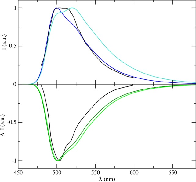
(Upper panel) Emission spectra of CQ in methanol as obtained by combining the ONIOM/EE-PMM procedure outcome with AH|FC (blue line) and AH|FCHT (cyan line) models to simulate the vibronic coupling; the corresponding experimental spectrum is also reported (black line). (Lower panel) CPL spectra of CQ in methanol as obtained by combining the ONIOM/EE-PMM procedure outcome with AH|FC (dark green line) and AH|FCHT (light green line) models to simulate the vibronic coupling, the corresponding experimental spectrum is also reported (black line).

Emission and CPL spectra show remarkable differences in their band shapes that are well reproduced in our simulations. Looking closer to the results, the experimental OPE (fluorescence) spectrum is characterized by two peaks with almost the same intensity. As already reported,⁸⁶ the two most intense peaks in the spectrum arise from different vibronic contributions. Bearing this in mind, the choice of the vibronic model is expected to have a high impact on the final spectra. In fact, it can be seen that while the AH|FC spectrum reduced to a shoulder the low-energy band, the inclusion of the HT term in the AH|FCHT spectrum overestimates its intensity. This behavior is present in the pure vibronic spectrum (see Figure S7 in SI) and has also been observed in the phosphorescence case.⁵³ As reported in Figure 8, a proper account of the solvent effects by the mean of the overall ONIOM/EE-PMM procedure modulates the HT contributions and, in turn, improves the overall agreement with the experimental spectrum reducing the second band prominence. The results of the CPL simulation are remarkable, and once again, they support our choice of perturbing only the electric transition dipole moment. The role of HT contributions in the CPL spectrum is less evident than in its OPE counterpart, although HT terms increase the intensity of the shoulder at 560 nm, which is clearly present in the experimental spectrum. In general, the remarkable matching between our computational data and the experimental results confirms the reliability and accuracy of our procedure also for the emission spectra.

4. Conclusion

With the present contribution we aimed to introduce and validate a cheap yet accurate multistep procedure to achieve an unbiased description of different spectroscopic phenomena occurring in condensed phases. By adding the outcomes of different computational methods, we were able to model vibrationally resolved absorption and emission spectra. As a test case, we choose a system characterized by chiroptical properties (namely, the camphorquinone dye in methanol solution) thus allowing us to test our procedure also in connection with the challenging reproduction of dichroic spectra. The starting point was the collection of “simple” results that, when properly combined, allowed us to get the refined final results. Namely, we started from (i) the collection of transition energies and dipole moments accounting for the effects of the interactions between the chromophore and the embedding environment as provided by MD simulations and (ii) the description of the vibrational modulation effects on the electronic transition involved, obtained by averaging the solvation effects through a continuum model. For the latter, we made use of a general computational tool implemented by one of the present authors in the Gaussian package, which is based on the Franck–Condon principle and provides different approximations for the vibronic contributions. For computing the effects of the chromophore–environment interactions we employed the recently proposed ONIOM/EE-PMM hybrid procedure²⁹ that combines the variational approach of the Electronic Embedding scheme within the ONIOM framework, with the perturbative approach formalized by the Perturbed Matrix Method. This procedure allows us to strongly reduce the need for a statistically significant number of solute–solvent configurations for the QM level calculations without any significant accuracy loss. In fact, for this rigid system we needed only one QM calculation to apply the procedure. This means that with a total number of two QM calculations (i.e., the one needed for the ONIOM/EE-PMM procedure plus the vibronic contribution calculation) we were able to fully model all the spectra issuing from absorption and emission possibly employing circularly polarized light. Moreover, the good agreement between all the computational results and their experimental counterparts, gives confidence about the robustness and reliability of the overall procedure. The performance of the new model for more challenging systems, especially flexible chromophores, will be investigated in forthcoming papers.

Supporting Information Available

The Supporting Information is available free of charge at https://pubs.acs.org/doi/10.1021/acs.jctc.0c00124.

• RESP and CM5 atomic charges; PCM vibronic spectra, shift vectors, and Duschinsky matrix representations; optimized CQ structures in XYZ format (PDF)

Author Contributions

^‡ S.D.G. and M.F. contributed equally to this work.

The authors declare no competing financial interest.

References

- Berova N.; Polavarapu P. L.; Nakanishi K.; Woody R. W.. Comprehensive chiroptical spectroscopy: applications in stereochemical analysis of synthetic compounds, natural products, and biomolecules; John Wiley & Sons, 2012; Vol. 2. [Google Scholar]
- McConnell O.; Bach A. II; Balibar C.; Byrne N.; Cai Y.; Carter G.; Chlenov M.; Di L.; Fan K.; Goljer I.; He Y.; Herold D.; Kagan M.; Kerns E.; Koehn F.; Kraml C.; Marathias V.; Marquez B.; McDonald L.; Nogle L.; Petucci C.; Schlingmann G.; Tawa G.; Tischler M.; Williamson R. T.; Sutherland A.; Watts W.; Young M.; Zhang M.-Y.; Zhang Y.; Zhou D.; Ho D. Enantiomeric separation and determination of absolute stereochemistry of asymmetric molecules in drug discovery—Building chiral technology toolboxes. Chirality 2007, 19, 658–682. 10.1002/chir.20399. [DOI] [PubMed] [Google Scholar]
- Gladiali S.; Alberico E. Asymmetric transfer hydrogenation: chiral ligands and applications. Chem. Soc. Rev. 2006, 35, 226–236. 10.1039/B513396C. [DOI] [PubMed] [Google Scholar]
- Berova N.; Nakanishi K.; Woody R. W.. Circular dichroism: principles and applications; John Wiley & Sons, 2000. [Google Scholar]
- Puzzarini C.; Bloino J.; Tasinato N.; Barone V. Accuracy and Interpretability: The Devil and the Holy Grail. New Routes Across Old Boundaries in Computational Spectroscopy. Chem. Rev. 2019, 119, 8131–8191. 10.1021/acs.chemrev.9b00007. [DOI] [PubMed] [Google Scholar]
- Barone V.; Baiardi A.; Bloino J. New Developments of a Multifrequency Virtual Spectrometer: Stereo-Electronic, Dynamical, and Environmental Effects on Chiroptical Spectra. Chirality 2014, 26, 588–600. 10.1002/chir.22325. [DOI] [PMC free article] [PubMed] [Google Scholar]
- Barone V. The virtual multifrequency spectrometer: a new paradigm for spectroscopy. WIREs Comput. Mol. Sci. 2016, 6, 86–110. 10.1002/wcms.1238. [DOI] [PMC free article] [PubMed] [Google Scholar]
- Morzan U. N.; Alonso de Armiño D. J.; Foglia N. O.; Ramñrez F.; González Lebrero M. C.; Scherlis D. A.; Estrin D. A. Spectroscopy in Complex Environments from QM–MM Simulations. Chem. Rev. 2018, 118, 4071–4113. 10.1021/acs.chemrev.8b00026. [DOI] [PubMed] [Google Scholar]
- Car R.; Parrinello M. Unified Approach for Molecular Dynamics and Density-Functional Theory. Phys. Rev. Lett. 1985, 55, 2471–2474. 10.1103/PhysRevLett.55.2471. [DOI] [PubMed] [Google Scholar]
- Frenkel D.; Smit B.. Understanding molecular simulation: from algorithms to applications; Elsevier, 2001; Vol. 1. [Google Scholar]
- a Levitt M. Birth and Future of Multiscale Modeling for Macromolecular Systems (Nobel Lecture). Angew. Chem., Int. Ed. 2014, 53, 10006–10018. 10.1002/anie.201403691. [DOI] [PubMed] [Google Scholar]; b Karplus M. Development of Multiscale Models for Complex Chemical Systems: From H+H2 to Biomolecules (Nobel Lecture). Angew. Chem., Int. Ed. 2014, 53, 9992–10005. 10.1002/anie.201403924. [DOI] [PubMed] [Google Scholar]; c Warshel A. Multiscale Modeling of Biological Functions: From Enzymes to Molecular Machines (Nobel Lecture). Angew. Chem., Int. Ed. 2014, 53, 10020–10031. 10.1002/anie.201403689. [DOI] [PMC free article] [PubMed] [Google Scholar]
- Chung L. W.; Sameera W. M. C.; Ramozzi R.; Page A. J.; Hatanaka M.; Petrova G. P.; Harris T. V.; Li X.; Ke Z.; Liu F.; Li H.; Ding L.; Morokuma K. The ONIOM Method and Its Applications. Chem. Rev. 2015, 115, 5678–5796. 10.1021/cr5004419. [DOI] [PubMed] [Google Scholar]
- Cisneros G. A.; Karttunen M.; Ren P.; Sagui C. Classical Electrostatics for Biomolecular Simulations. Chem. Rev. 2014, 114, 779–814. 10.1021/cr300461d. [DOI] [PMC free article] [PubMed] [Google Scholar]
- Lin H.; Truhlar D. G. QM/MM: what have we learned, where are we, and where do we go from here?. Theor. Chem. Acc. 2007, 117, 185. 10.1007/s00214-006-0143-z. [DOI] [Google Scholar]
- Senn H. M.; Thiel W. QM/MM Methods for Biomolecular Systems. Angew. Chem., Int. Ed. 2009, 48, 1198–1229. 10.1002/anie.200802019. [DOI] [PubMed] [Google Scholar]
- Rosa M.; Micciarelli M.; Laio A.; Baroni S. Sampling Molecular Conformers in Solution with Quantum Mechanical Accuracy at a Nearly Molecular-Mechanics Cost. J. Chem. Theory Comput. 2016, 12, 4385–4389. 10.1021/acs.jctc.6b00470. [DOI] [PubMed] [Google Scholar]
- Zuehlsdorff T. J.; Isborn C. M. Combining the ensemble and Franck-Condon approaches for calculating spectral shapes of molecules in solution. J. Chem. Phys. 2018, 148, 024110. 10.1063/1.5006043. [DOI] [PubMed] [Google Scholar]
- Stephens P. J.; Devlin F. J.; Cheeseman J. R.. VCD spectroscopy for organic chemists; CRC Press, 2012. [Google Scholar]
- Stephens P. J.; Devlin F. J.; Chabalowski C. F.; Frisch M. J. Ab Initio Calculation of Vibrational Absorption and Circular Dichroism Spectra Using Density Functional Force Fields. J. Phys. Chem. 1994, 98, 11623–11627. 10.1021/j100096a001. [DOI] [Google Scholar]
- Autschbach J. Computing chiroptical properties with first-principles theoretical methods: Background and illustrative examples. Chirality 2009, 21, E116–E152. 10.1002/chir.20789. [DOI] [PubMed] [Google Scholar]
- Pecul M.; Ruud K. In Continuum Solvation Models in Chemical Physics:Physics: From Theory to Applications; Mennucci B., Cammi R., Eds.; John Wiley & Sons, Ltd, 2007; Chapter 2, pp 206–219. [Google Scholar]
- Pecul M. In Comprehensive Chiroptical Spectroscopy; Berova N., Polavarapu P. L., Nakanishi K., Woody R. W., Eds.; John Wiley & Sons, Ltd, 2012; Chapter 25, pp 729–745. [Google Scholar]
- Berova N.; Polavarapu P. L.; Nakanishi K.; Woody R. W.. Comprehensive Chiroptical Spectroscopy: Instrumentation, Methodologies, and Theoretical Simulations; John Wiley & Sons, 2011; Vol. 1. [Google Scholar]
- Crawford T. D.; Stephens P. J. Comparison of Time-Dependent Density-Functional Theory and Coupled Cluster Theory for the Calculation of the Optical Rotations of Chiral Molecules. J. Phys. Chem. A 2008, 112, 1339–1345. 10.1021/jp0774488. [DOI] [PubMed] [Google Scholar]
- Srebro M.; Govind N.; de Jong W. A.; Autschbach J. Optical Rotation Calculated with Time-Dependent Density Functional Theory: The OR45 Benchmark. J. Phys. Chem. A 2011, 115, 10930–10949. 10.1021/jp2055409. [DOI] [PubMed] [Google Scholar]
- Wiberg K. B.; Caricato M.; Wang Y.-G.; Vaccaro P. H. Towards the Accurate and Efficient Calculation of Optical Rotatory Dispersion Using Augmented Minimal Basis Sets. Chirality 2013, 25, 606–616. 10.1002/chir.22184. [DOI] [PubMed] [Google Scholar]
- McAlexander H. R.; Mach T. J.; Crawford T. D. Localized optimized orbitals, coupled cluster theory, and chiroptical response properties. Phys. Chem. Chem. Phys. 2012, 14, 7830–7836. 10.1039/c2cp23797k. [DOI] [PubMed] [Google Scholar]
- McAlexander H. R.; Crawford T. D. A Comparison of Three Approaches to the Reduced-Scaling Coupled Cluster Treatment of Non-Resonant Molecular Response Properties. J. Chem. Theory Comput. 2016, 12, 209–222. 10.1021/acs.jctc.5b00898. [DOI] [PubMed] [Google Scholar]
- Del Galdo S.; Chandramouli B.; Mancini G.; Barone V. Assessment of Multi-Scale Approaches for Computing UV–Vis Spectra in Condensed Phases: Toward an Effective yet Reliable Integration of Variational and Perturbative QM/MM Approaches. J. Chem. Theory Comput. 2019, 15, 3170–3184. 10.1021/acs.jctc.9b00120. [DOI] [PubMed] [Google Scholar]
- Dapprich S.; Komáromi I.; Byun K.; Morokuma K.; Frisch M. J. A new ONIOM implementation in Gaussian98. Part I. The calculation of energies, gradients, vibrational frequencies and electric field derivatives. J. Mol. Struct.: THEOCHEM 1999, 461–462, 1–21. 10.1016/S0166-1280(98)00475-8. [DOI] [Google Scholar]
- Vreven T.; Byun K. S.; Komàromi I.; Dapprich S.; Montgomery J. A. Jr.; Morokuma K.; Frisch M. J. Combining Quantum Mechanics Methods with Molecular Mechanics Methods in ONIOM. J. Chem. Theory Comput. 2006, 2, 815–826. 10.1021/ct050289g. [DOI] [PubMed] [Google Scholar]
- Aschi M.; Spezia R.; Nola A. D.; Amadei A. A first-principles method to model perturbed electronic wavefunctions: the effect of an external homogeneous electric field. Chem. Phys. Lett. 2001, 344, 374–380. 10.1016/S0009-2614(01)00638-8. [DOI] [Google Scholar]
- Spezia R.; Aschi M.; Di Nola A.; Amadei A. Extension of the perturbed matrix method: application to a water molecule. Chem. Phys. Lett. 2002, 365, 450–456. [Google Scholar]
- Carrillo-Parramon O.; Del Galdo S.; Aschi M.; Mancini G.; Amadei A.; Barone V. Flexible and Comprehensive Implementation of MD-PMM Approach in a General and Robust Code. J. Chem. Theory Comput. 2017, 13, 5506–5514. 10.1021/acs.jctc.7b00341. [DOI] [PubMed] [Google Scholar]
- Shao J.; Tanner S. W.; Thompson N.; Cheatham T. E. Clustering Molecular Dynamics Trajectories: 1. Characterizing the Performance of Different Clustering Algorithms. J. Chem. Theory Comput. 2007, 3, 2312–2334. 10.1021/ct700119m. [DOI] [PubMed] [Google Scholar]
- Kessler J.; Dračínskỳ M.; Bouř P. Parallel variable selection of molecular dynamics clusters as a tool for calculation of spectroscopic properties. J. Comput. Chem. 2013, 34, 366–371. 10.1002/jcc.23143. [DOI] [PubMed] [Google Scholar]
- Daura X.; Bakowies D.; Seebach D.; Fleischhauer J.; Van Gunsteren W. F.; Krüger P. Circular dichroism spectra of β-peptides: sensitivity to molecular structure and effects of motional averaging. Eur. Biophys. J. 2003, 32, 661–670. 10.1007/s00249-003-0303-1. [DOI] [PubMed] [Google Scholar]
- Del Galdo S.; Mancini G.; Daidone I.; Zanetti Polzi L.; Amadei A.; Barone V. Tyrosine absorption spectroscopy: Backbone protonation effects on the side chain electronic properties. J. Comput. Chem. 2018, 39, 1747–1756. 10.1002/jcc.25351. [DOI] [PubMed] [Google Scholar]
- Bloino J.; Biczysko M.; Santoro F.; Barone V. General Approach to Compute Vibrationally Resolved One-Photon Electronic Spectra. J. Chem. Theory Comput. 2010, 6, 1256–1274. 10.1021/ct9006772. [DOI] [PubMed] [Google Scholar]
- Luk C. K.; Richardson F. S. Circularly polarized luminescence spectrum of camphorquinone. J. Am. Chem. Soc. 1974, 96, 2006–2009. 10.1021/ja00814a004. [DOI] [Google Scholar]
- Steinberg N.; Gafni A.; Steinberg I. Z. Measurement of the optical activity of triplet-singlet transitions. The circular polarization of phosphorescence of camphorquinone and benzophenone. J. Am. Chem. Soc. 1981, 103, 1636–1640. 10.1021/ja00397a006. [DOI] [Google Scholar]
- Romani A.; Favaro G.; Masetti F. Luminescence properties of camphorquinone at room temperature. J. Lumin. 1995, 63, 183–188. 10.1016/0022-2313(94)00066-L. [DOI] [Google Scholar]
- Longhi G.; Castiglioni E.; Abbate S.; Lebon F.; Lightner D. A. Experimental and Calculated CPL Spectra and Related Spectroscopic Data of Camphor and Other Simple Chiral Bicyclic Ketones. Chirality 2013, 25, 589–599. 10.1002/chir.22176. [DOI] [PubMed] [Google Scholar]
- Pritchard B.; Autschbach J. Calculation of the Vibrationally Resolved, Circularly Polarized Luminescence of d-Camphorquinone and (S,S)-trans-β-Hydrindanone. ChemPhysChem 2010, 11, 2409–2415. 10.1002/cphc.201000054. [DOI] [PubMed] [Google Scholar]
- Berendsen H.J.C.; van der Spoel D.; van Drunen R. GROMACS: A message-passing parallel molecular dynamics implementation. Comput. Phys. Commun. 1995, 91, 43–56. [Google Scholar]
- Bayly C. I.; Cieplak P.; Cornell W. D.; Kollman P. A. A Well-Behaved Electrostatic Potential Based Method Using Charge Restraints for Deriving Atomic Charges: The RESP Model. J. Phys. Chem. 1993, 97, 10269–10280. 10.1021/j100142a004. [DOI] [Google Scholar]
- Schmid N.; Eichenberger A. P.; Choutko A.; Riniker S.; Winger M.; Mark A. E.; van Gunsteren W. F. Definition and testing of the GROMOS force-field versions 54A7 and 54B7. Eur. Biophys. J. 2011, 40, 843. 10.1007/s00249-011-0700-9. [DOI] [PubMed] [Google Scholar]
- Lee C.; Yang W.; Parr R. G. Development of the Colle-Salvetti correlation-energy formula into a functional of the electron density. Phys. Rev. B: Condens. Matter Mater. Phys. 1988, 37, 785–789. 10.1103/PhysRevB.37.785. [DOI] [PubMed] [Google Scholar]
- Becke A. D. Density-functional exchange-energy approximation with correct asymptotic behavior. Phys. Rev. A: At., Mol., Opt. Phys. 1988, 38, 3098–3100. 10.1103/PhysRevA.38.3098. [DOI] [PubMed] [Google Scholar]
- Lee C.; Yang W.; Parr R. G. Development of the Colle-Salvetti Correlation-Energy Formula into a Functional of the Electron Density. Phys. Rev. B: Condens. Matter Mater. Phys. 1988, 37, 785–789. 10.1103/PhysRevB.37.785. [DOI] [PubMed] [Google Scholar]
- Dunning T. H. Gaussian basis sets for use in correlated molecular calculations. I. The atoms boron through neon and hydrogen. J. Chem. Phys. 1989, 90, 1007–1023. 10.1063/1.456153. [DOI] [Google Scholar]
- Frisch M. J.; Trucks G. W.; Schlegel H. B.; Scuseria G. E.; Robb M. A.; Cheeseman J. R.; Scalmani G.; Barone V.; Petersson G. A.; Nakatsuji H.; Li X.; Caricato M.; Marenich A. V.; Bloino J.; Janesko B. G.; Gomperts R.; Mennucci B.; Hratchian H. P.; Ortiz J. V.; Izmaylov A. F.; Sonnenberg J. L.; Williams-Young D.; Ding F.; Lipparini F.; Egidi F.; Goings J.; Peng B.; Petrone A.; Henderson T.; Ranasinghe D.; Zakrzewski V. G.; Gao J.; Rega N.; Zheng G.; Liang W.; Hada M.; Ehara M.; Toyota K.; Fukuda R.; Hasegawa J.; Ishida M.; Nakajima T.; Honda Y.; Kitao O.; Nakai H.; Vreven T.; Throssell K.; Montgomery J. A. Jr.; Peralta J. E.; Ogliaro F.; Bearpark M. J.; Heyd J. J.; Brothers E. N.; Kudin K. N.; Staroverov V. N.; Keith T. A.; Kobayashi R.; Normand J.; Raghavachari K.; Rendell A. P.; Burant J. C.; Iyengar S. S.; Tomasi J.; Cossi M.; Millam J. M.; Klene M.; Adamo C.; Cammi R.; Ochterski J. W.; Martin R. L.; Morokuma K.; Farkas O.; Foresman J. B.; Fox D. J.. Gaussian 16, Revision B.01; Gaussian Inc.: Wallingford, CT, 2016.
- Egidi F.; Fusè M.; Baiardi A.; Bloino J.; Li X.; Barone V. Computational simulation of vibrationally resolved spectra for spin-forbidden transitions. Chirality 2018, 30, 850–865. 10.1002/chir.22864. [DOI] [PMC free article] [PubMed] [Google Scholar]
- Mennucci B. Polarizable Continuum Model. WIREs Comput. Mol. Sci. 2012, 2, 386–404. 10.1002/wcms.1086. [DOI] [Google Scholar]
- Cappelli C.; Bloino J.; Lipparini F.; Barone V. Toward Ab Initio Anharmonic Vibrational Circular Dichroism Spectra in the Condensed Phase. J. Phys. Chem. Lett. 2012, 3, 1766–1773. 10.1021/jz3006139. [DOI] [PubMed] [Google Scholar]
- Jorgensen W. L.; Maxwell D. S.; Tirado-Rives J. Development and Testing of the OPLS All-Atom Force Field on Conformational Energetics and Properties of Organic Liquids. J. Am. Chem. Soc. 1996, 118, 11225–11236. 10.1021/ja9621760. [DOI] [Google Scholar]
- Bussi G.; Donadio D.; Parrinello M.. Canonical sampling through velocity rescaling. J. Chem. Phys. 2007, 126.014101. 10.1063/1.2408420 [DOI] [PubMed] [Google Scholar]
- Hess B.; Bekker H.; Berendsen H. J. C.; Fraaije J. G. E. M. LINCS: A linear constraint solver for molecular simulations. J. Comput. Chem. 1997, 18, 1463–1472. . [DOI] [Google Scholar]
- Darden T.; York D.; Pedersen L. Particle mesh Ewald: An N-log(N) method for Ewald sums in large systems. J. Chem. Phys. 1993, 98, 10089. 10.1063/1.464397. [DOI] [Google Scholar]
- Goodwin R. D. Methanol Thermodynamic Properties From 176 to 673 K at Pressures to 700 bar. J. Phys. Chem. Ref. Data 1987, 16, 799–892. 10.1063/1.555786. [DOI] [Google Scholar]
- Macchiagodena M.; Mancini G.; Pagliai M.; Barone V. Accurate prediction of bulk properties in hydrogen bonded liquids: amides as case studies. Phys. Chem. Chem. Phys. 2016, 18, 25342–25354. 10.1039/C6CP04666E. [DOI] [PubMed] [Google Scholar]
- Pagliai M.; Raugei S.; Cardini G.; Schettino V. Hydrogen bond dynamics in liquid methanol. J. Chem. Phys. 2003, 119, 6655. 10.1063/1.1605093. [DOI] [Google Scholar]
- Marenich A. V.; Jerome S. V.; Cramer C. J.; Truhlar D. G. Charge Model 5: An extension of Hirshfeld Population Analysis for the accurate description of molecular interactions in gaseous and condensed phases. J. Chem. Theory Comput. 2012, 8, 527–541. 10.1021/ct200866d. [DOI] [PubMed] [Google Scholar]
- Brunk E.; Rothlisberger U. Mixed Quantum Mechanical/Molecular Mechanical Molecular Dynamics Simulations of Biological Systems in Ground and Electronically Excited States. Chem. Rev. 2015, 115, 6217–6263. 10.1021/cr500628b. [DOI] [PubMed] [Google Scholar]
- Gross E.; Dobson J.; Petersilka M. Density functional theory of time-dependent phenomena. Top. Curr. Chem. 1996, 181, 81. 10.1007/BFb0016643. [DOI] [Google Scholar]
- Krishnan R.; Binkley J. S.; Seeger R.; Pople J. A.. Self-consistent molecular orbital methods. XX. A basis set for correlated wave functions. J. Chem. Phys. 1980, 72.650. 10.1063/1.438955 [DOI] [Google Scholar]
- Zanetti-Polzi L.; Del Galdo S.; Daidone I.; D’Abramo M.; Barone V.; Aschi M.; Amadei A. Extending the perturbed matrix method beyond the dipolar approximation: comparison of different levels of theory. Phys. Chem. Chem. Phys. 2018, 20, 24369–24378. 10.1039/C8CP04190C. [DOI] [PubMed] [Google Scholar]
- Mancini G.; Brancato G.; Chandramouli B.; Barone V. Organic solvent simulations under non-periodic boundary conditions: A library of effective potentials for the GLOB model. Chem. Phys. Lett. 2015, 625, 186–192. 10.1016/j.cplett.2015.03.001. [DOI] [Google Scholar]
- Kongsted J.; Mennucci B.; Coutinho K.; Canuto S. Solvent effects on the electronic absorption spectrum of camphor using continuum, discrete or explicit approaches. Chem. Phys. Lett. 2010, 484, 185–191. 10.1016/j.cplett.2009.11.026. [DOI] [Google Scholar]
- Barone V.; Bloino J.; Biczysko M.; Santoro F. Fully Integrated Approach to Compute Vibrationally Resolved Optical Spectra: From Small Molecules to Macrosystems. J. Chem. Theory Comput. 2009, 5, 540–554. 10.1021/ct8004744. [DOI] [PubMed] [Google Scholar]
- Bloino J.; Baiardi A.; Biczysko M. Aiming at an accurate prediction of vibrational and electronic spectra for medium-to-large molecules: An overview. Int. J. Quantum Chem. 2016, 116, 1543–1574. 10.1002/qua.25188. [DOI] [Google Scholar]
- Duschinsky F. The importance of the electron spectrum in multi atomic molecules. Concerning the Franck-Condon principle. Acta Physicochim. URSS 1937, 7, 551–566. [Google Scholar]
- de Oliveira D. C. R. S.; Rocha M. G.; Gatti A.; Correr A. B.; Ferracane J. L.; Sinhoret M. A. C. Effect of different photoinitiators and reducing agents on cure efficiency and color stability of resin-based composites using different LED wavelengths. J. Dent. 2015, 43, 1565–1572. 10.1016/j.jdent.2015.08.015. [DOI] [PubMed] [Google Scholar]
- Okulus Z.; Buchwald T.; Szybowicz M.; Voelkel A. Study of a new resin-based composites containing hydroxyapatite filler using Raman and infrared spectroscopy. Mater. Chem. Phys. 2014, 145, 304–312. 10.1016/j.matchemphys.2014.02.012. [DOI] [Google Scholar]
- Ikemura K.; Endo T.. A review of the development of radical photopolymerization initiators used for designing light-curing dental adhesives and resin composites. Dent. Mater. J. 2010, advpub, 29, 481–501. 10.4012/dmj.2009-137 [DOI] [PubMed] [Google Scholar]
- Goerigk L.; Grimme S. Efficient and Accurate Double-Hybrid-Meta-GGA Density Functionals–Evaluation with the Extended GMTKN30 Database for General Main Group Thermochemistry, Kinetics, and Noncovalent Interactions. J. Chem. Theory Comput. 2011, 7, 291–309. 10.1021/ct100466k. [DOI] [PubMed] [Google Scholar]
- Biczysko M.; Panek P.; Scalmani G.; Bloino J.; Barone V. Harmonic and Anharmonic Vibrational Frequency Calculations with the Double-Hybrid B2PLYP Method: Analytic Second Derivatives and Benchmark Studies. J. Chem. Theory Comput. 2010, 6, 2115–2125. 10.1021/ct100212p. [DOI] [PubMed] [Google Scholar]
- Fusè M.; Mazzeo G.; Longhi G.; Abbate S.; Masi M.; Evidente A.; Puzzarini C.; Barone V. Unbiased Determination of Absolute Configurations by vis-à-vis Comparison of Experimental and Simulated Spectra: The Challenging Case of Diplopyrone. J. Phys. Chem. B 2019, 123, 9230–9237. 10.1021/acs.jpcb.9b08375. [DOI] [PubMed] [Google Scholar]
- Grimme S.; Neese F. Double-hybrid density functional theory for excited electronic states of molecules. J. Chem. Phys. 2007, 127, 154116. 10.1063/1.2772854. [DOI] [PubMed] [Google Scholar]
- Jacquemin D.; Wathelet V.; Perpète E. A.; Adamo C. Extensive TD-DFT Benchmark: Singlet-Excited States of Organic Molecules. J. Chem. Theory Comput. 2009, 5, 2420–2435. 10.1021/ct900298e. [DOI] [PubMed] [Google Scholar]
- Laurent A. D.; Jacquemin D. TD-DFT benchmarks: A review. Int. J. Quantum Chem. 2013, 113, 2019–2039. 10.1002/qua.24438. [DOI] [Google Scholar]
- Papajak E.; Zheng J.; Xu X.; Leverentz H. R.; Truhlar D. G. Perspectives on Basis Sets Beautiful: Seasonal Plantings of Diffuse Basis Functions. J. Chem. Theory Comput. 2011, 7, 3027–3034. 10.1021/ct200106a. [DOI] [PubMed] [Google Scholar]
- Grimme S.; Ehrlich S.; Goerigk L. Effect of the Damping Function in Dispersion Corrected Density Functional Theory. J. Comput. Chem. 2011, 32, 1456–1465. 10.1002/jcc.21759. [DOI] [PubMed] [Google Scholar]
- Benassi E.; Cappelli C.; Carlotti B.; Barone V. An integrated computational tool to model the broadening of the absorption bands of flexible dyes in solution: cationic chromophores as test cases. Phys. Chem. Chem. Phys. 2014, 16, 26963–26973. 10.1039/C4CP03419H. [DOI] [PubMed] [Google Scholar]
Associated Data
This section collects any data citations, data availability statements, or supplementary materials included in this article.