Ultrastructural details of mammalian chromosome architecture

SUMMARY

Over the past decade, 3C-related methods have provided remarkable insights into chromosome folding in vivo. To overcome the limited resolution of prior studies, we extend a recently-developed Hi-C variant, Micro-C, to map chromosome architecture at nucleosome resolution in human ESCs and fibroblasts. Micro-C robustly captures known features of chromosome folding including compartment organization, topologically associating domains, and interactions between CTCF binding sites. In addition, Micro-C provides a detailed map of nucleosome positions, and localizes contact domain boundaries with nucleosomal precision. Compared to Hi-C, Micro-C exhibits an order of magnitude greater dynamic range, allowing the ~20,000 additional loops in each cell type. Many newly-identified peaks are localized along extrusion stripes and form transitive grids, consistent with their anchors being pause sites impeding cohesin-dependent loop extrusion. Our analyses comprise the highest resolution maps of chromosome folding in human cells to date, providing a valuable resource for studies of chromosome organization.

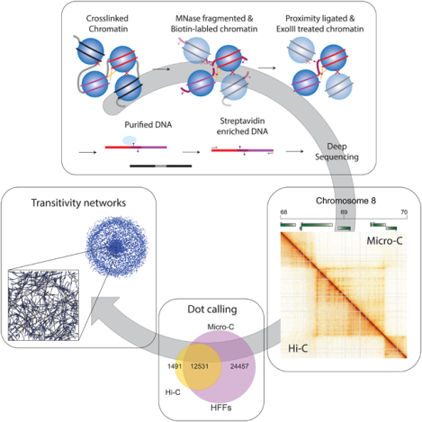
Graphical Abstract

eTOC:

Krietenstein et al. extend analyses of chromosome folding to nucleosome resolution in human cells. These ultra-deep Micro-C maps capture known features of chromosomes with improved signal-to-noise, identifying tens of thousands of new looping interactions. Newly-identified loops reveal weak pause sites along cohesin extrusion tracks, providing insight into TAD structural heterogeneity.

INTRODUCTION

The organization of the genome within the nucleus has wide-ranging effects on DNA-templated processes ranging from transcription to DNA repair. In eukaryotes, the one-dimensional packaging of chromatin into nucleosomes is understood in great detail, with genome-wide maps of nucleosome positions and composition available for a wide variety of organisms, often in many different growth conditions or for a variety of distinct cell types (Friedman and Rando, 2015; Lai and Pugh, 2017). Although our understanding of three-dimensional folding of the genome somewhat lags the 1D picture, over the past decade a wide variety of technical approaches have provided impressively concordant views of chromosome architecture in vivo, as for example chromosome compartments and TAD organization are readily captured using various chromosome conformation capture (3C) methods (Dixon et al., 2012; Lieberman-Aiden et al., 2009; Nora et al., 2012), microscopy-based methods (Boettiger et al., 2016; Finn et al., 2019), and orthogonal methods such as genome architecture mapping (Beagrie et al., 2017).

A number of organizing principles emerge from this burgeoning body of literature, which reveals that the folding of chromosomes in three-dimensional space is driven by at least four major processes: 1) At the scale of the nucleus, chromosomes occupy distinct territories, and are oriented by inter-chromosomal interactions between key genomic loci (eg telomere-telomere and centromere-centromere interactions in the Rabl configuration) as well as interactions between chromosomal loci and various subnuclear landmarks including the nucleolus, the nuclear lamina, and paraspeckles (Cremer and Cremer, 2010; Quinodoz et al., 2018; van Steensel and Belmont, 2017). 2) Chromosomes are next organized into megabase-scale regions that segregate into compartments, in which active genes associate with other active genes while repressed genes cluster together (Lieberman-Aiden et al., 2009). Compartment organization is thought to be at least partially driven by the process of phase separation, which is increasingly understood to be responsible for self-organization of subcellular organelles such as P granules or nucleoli (Falk et al., 2019; Larson et al., 2017; Shin and Brangwynne, 2017; Strom et al., 2017) – the heterochromatin protein HP1 for example exhibits phase separation properties both in vivo and in vitro. 3) At length scales on the order of 1–5 genes – ~100 kb to 1 Mb in mammals – chromosomes are organized into structural domains known as topologically associating domains (TADs) in most organisms, although seemingly analogous structures in bacteria and yeast have been termed chromosomally-interacting domains (CIDs) (Dixon et al., 2012; Hsieh et al., 2015; Le et al., 2013; Nora et al., 2012; Sexton et al., 2012). Organization of chromosomes into TADs is thought to be largely driven by ATP-dependent loop extrusion, in which the SMC-family ATPase cohesin is loaded onto DNA and pumps DNA on either side inwards until encountering a barrier, most often comprised of the sequence-specific DNA-binding protein CTCF (Fudenberg et al., 2017; Fudenberg et al., 2016; Nora et al., 2017; Rao et al., 2014; Rao et al., 2017). Signatures of the loop extrusion process in ensemble measurements include enriched interactions between two extrusion barriers (forming an off-diagonal dot in Hi-C contact maps), as well as “flares” emanating from individual barriers (resulting from an extruder encountering one barrier first while continuing to pump DNA into the other side of the loop). Within TADs, additional looping interactions occur, such as those between distal regulatory elements (enhancers) and gene promoters, although these loops are inconsistently observed even in extremely high-resolution Hi-C maps. 4) Finally, chromosome organization at the scale of 1–10 nucleosomes – the scale that would roughly correspond to secondary structure in protein folding – is dominated by the intrinsic affinity of nucleosomes for one another. In vitro and electron microscopy studies increasingly support the idea that nucleosomes form short stretches organized in a “zig-zag” orientation, with nucleosome N interacting preferentially with nucleosome N+2 (Dorigo et al., 2004; Grigoryev et al., 2009; Ou et al., 2017; Song et al., 2014; Yao et al., 1993). Although, at times, this zig-zag signal has been interpreted as supporting the idea of an extended secondary structural element known as the 30 nm fiber, a variety of recent studies strongly suggest that while a short tri- or tetranucleosome zig-zag motif may be prevalent in vivo (Grigoryev et al., 2009; Hsieh et al., 2015; Ohno et al., 2019; Ou et al., 2017; Ricci et al., 2015; Risca et al., 2017), this appears to be limited to short “clutches” of nucleosomes, with very little evidence supporting the idea of extended stretches of regular secondary structure in vivo.

The majority of genome-wide studies of chromosome folding utilize 3C-based proximity ligation methods (Dekker et al., 2002), in which genomic loci in physical proximity are covalently crosslinked to one another, chromatin is fragmented using restriction enzymes, and interacting genomic loci are then identified following ligation and paired-end deep sequencing. The fundamental resolution of chromosome conformation capture is largely defined by the size and uniformity of chromatin fragmentation prior to proximity ligation. To approach the maximum practical resolution to 3C methods, which is set by the ubiquitous packaging of the genome into repeating nucleosomal units (Van Holde, 1989), we recently developed Micro-C, a Hi-C protocol in which chromatin is fragmented to mononucleosomes using micrococcal nuclease (MNase), thereby increasing both fragment density as well as uniformity of spacing (Hsieh et al., 2015; Hsieh et al., 2016). Although a substantially updated version of this protocol with an additional crosslinking step and improved signal-to-noise was originally named Micro-C XL (Hsieh et al., 2016), given that this protocol completely supersedes the original one we will simply refer to the updated protocol as Micro-C throughout. The Micro-C protocols were developed in budding and fission yeast, and provide insight into chromosome folding at scales ranging from single nucleosomes to the entire genome.

Here, we sought to enhance the resolution of mammalian chromosome folding studies by applying Micro-C to two human cell types – pluripotent H1 embryonic stem cells, and human foreskin fibroblasts (HFFs). Micro-C maps readily captured known features of both 1D and 3D chromosome folding, with nucleosome positioning maps, A/B compartments, TAD locations, and loops between convergently oriented CTCF-binding sites all concordant with previous studies. Moreover, Micro-C maps exhibited significantly improved signal-to-noise relative to Hi-C maps of the same cell lines, enabling the identification of previously unappreciated features of mammalian chromosome architecture. Most dramatically, we identified ~3–5 times more looping interactions in our Micro-C maps than in comparable Hi-C maps, with many of the newly-identified loops bridging regulatory elements. Our data support the utility of MicroC for analysis of chromosome folding at unprecedented resolution, and provide novel insights into multiple aspects of chromosome organization in mammals.

RESULTS

Generation of matched Micro-C and Hi-C maps in two human cell lines

To extend our Micro-C analysis of chromosome folding from the relatively simple yeast genome to the more complex chromosomal organization seen in mammals, we generated deeply-sequenced Micro-C datasets (~2.6–4.5 billion uniquely mapped reads per sample, ~150X coverage per nucleosome – Table S1) for two well-studied human cell types: pluripotent human embryonic stem cells (H1-ESC) and differentiated human foreskin fibroblasts (HFFc6). Supplementary Figure S1A shows typical examples of MNase digestion to ~90% mononucleosomes prior to ligation, along with the subsequent production of dinucleosome-sized ligation products between crosslinked nucleosomes. To benchmark our approach, we also generated Hi-C datasets for these two cell types in parallel, following the in situ Hi-C protocol with a 4 bp cutter (DpnII) (Belaghzal et al., 2017).

To visually compare Hi-C and Micro-C views of human cells, we plotted contact heatmaps for ESCs and HFFs in Figures 1A–B at four scales arranged from chromosome-scale (left) to single-gene resolution (right). Overall, Micro-C and Hi-C maps reveal the same major classes of patterns that illuminate various features of chromosome folding: at lower resolutions (e.g, ~25 kb bins) the coarse checkerboard pattern reflects the compartmentalization of active and inactive chromatin, while zooming to higher resolutions (e.g. <10 kb bins) reveals finer compartmental segmentation, TADs, and off-diagonal interaction peaks thought to result from a high frequency of CTCF-anchored long-range looping interactions.

Figure 1. Micro-C of human pluripotent and differentiated cell types recovers coarse features of chromosome folding.

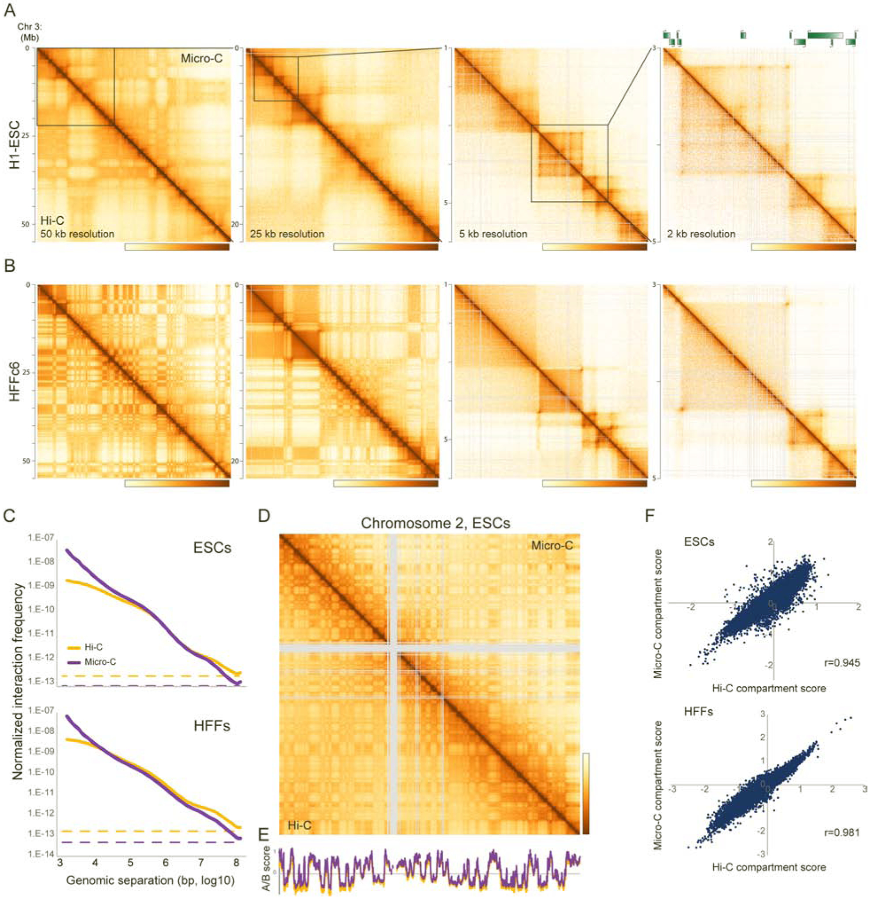
(A-B) Chromosome contact maps for four successive zoom-ins across human chromosome 3, for H1 ESCs (A) and HFFs (B). Each panel shows Micro-C data above the diagonal, with Hi-C data for the same cell line below the diagonal. All four datasets represent two biological replicates, with technical replicate numbers provided in Table S1. Here, and for all other contact maps throughout the manuscript, color scale is set to saturate at no detectable interactions (yellow) to the 99^th percentile of interaction values (brown) in the selected region.

(C) Interaction frequency is plotted for Micro-C and Hi-C on the y axis as a function of genomic distance between interacting fragments (x axis), for ESCs and HFFs. Both axes are in log₁₀ scale. In both cases, dotted lines show the genome-wide average interaction frequency between loci located on different chromosomes, an estimate of nonspecific dataset noise. See also Supplementary Figures S1B–D.

(D) Micro-C robustly captures A/B compartment organization. Heatmap shows Hi-C and Micro-C interaction maps (binned at 100 kb resolution) for Chromosome 2 in ESCs, illustrating the nearly identical A/B “checkerboard” pattern captured by both methods. See also Supplementary Figure S2.

(E) Eigenvector scores for chromosome 2 in ESCs compared for the Hi-C dataset (orange) vs. the Micro-C dataset (purple).

(F) Eigenvector scores are globally correlated between Hi-C and Micro-C maps. Scatterplots show A/B scores for 100 kb genomic tiles in Hi-C (x axis) vs. Micro-C (y axis) maps of ESCs and HFFs.

Micro-C exhibits improved signal-to-noise relative to Hi-C

To broadly survey the performance of Micro-C relative to Hi-C methods, we examined the scaling of contact frequency P(s) as a function of the distance between two genomic loci. Comparing Hi-C and Micro-C, we find a similar decay in interactions with increasing distance for length scales from ~20,000 bp to 1 Mb (Figure 1C, Supplementary Figure S1B). However, Micro-C exhibits an increased dynamic range of contact frequency, with improvements at both small and large genomic separations. At large separations (>10 Mb), where contacts are expected to be very rare, P(s) curves flatten to approximately the levels of interchromosomal contact frequency (Figure 1C), which is 2 to 3-fold lower in Micro-C than in Hi-C. This was not a result of differences in sequencing depth, as we observed the same phenomenon in datasets downsampled to yield equivalent numbers of cis-interacting read pairs (Supplementary Figure S1C). Moreover, the relative dearth of long-range interactions in Micro-C was not entirely a result of the increased frequency of short-range interactions, as renormalizing the dataset following removal of interactions below 10 kb did not eliminate the difference between Hi-C and Micro-C for long-range interactions (Supplementary Figure S1D). Instead, we believe the average reduction in both interchromosomal and extremely long-range intrachromosomal contact frequencies observed in Micro-C is likely due in part to lowering of the “noise floor” of artifactual contacts (random ligations between unlinked nucleosomes) (Hsieh et al., 2016).

At shorter scales, Micro-C consistently recovers a higher fraction of close-range near-diagonal contacts, providing greater coverage of short-range chromosome folding behaviors at the 1–100 nucleosome scale (Figure 1C, Supplementary Figure S1E). This length scale includes the 1–5 nucleosome scale (Supplementary Figures S1F–G) that is inaccessible to traditional Hi-C due to the longer average fragment size (~400 bp on average for DpnII digestion, with actual fragment sizes closer to ~1 kb in practice due to partial digestion) and the heterogeneity of fragment lengths resulting from uneven spacing of restriction sites (Supplementary Figure S1H). Importantly, this length scale, along with the fact that the protocol explicitly captures interactions between mononucleosomes, has the potential to provide information about the arrangement and interactions of nucleosomal arrays and about chromatin fiber structure (Risca et al., 2017).

At low and intermediate resolution, Micro-C data recapitulates the chromosome organization seen in Hi-C maps. For example, A/B compartment calls are strongly correlated (r=0.945 and 0.981 for ESCs and HFFs, respectively, at 100 kb resolution) between Micro-C and Hi-C maps (Figure 1D–F). Although many compartments encompass relatively large (~1 Mb) genomic intervals, consistent with prior reports (Rowley et al., 2017) we also find many examples of extremely fine single-gene scale compartments (exhibiting the “plaid” pattern typical of compartments and thus distinct from TADs) in both cell types (Supplementary Figure S2A). Intriguingly, we find a dramatic increase in compartment strength in fibroblasts in both datasets (Supplementary Figure S2B), presumably reflecting both the unusually short G1 phase of the ES cell cycle, as well as increased regulatory specialization observed as cells differentiate. In addition to this global change in the overall strength of genomic compartmentalization, we find predictable changes in compartment organization of individual genes as they are differentially induced or repressed in the two cell types – genes upregulated in HFFs generally switch from repressive to active compartments, and vice versa (Supplementary Figures S2C–D).

While Micro-C and Hi-C maps therefore provide highly concordant views at the coarsest level of genomic organization, they are clearly distinct at higher resolution, as for example a number of interaction peaks (“dots”) are apparent in the Micro-C dataset that are absent in Hi-C, as described in detail below.

Nucleosome positioning and short-range internucleosomal interactions

One unique feature of the Micro-C protocol, compared to restriction enzyme-based 3C methods, is that all interacting chromatin fragments are mononucleosomes. As a result, ignoring read pairs and treating the dataset as a single-end MNase-Seq dataset provides a genome-wide map of nucleosomes for a given cell type “for free” (with the possible caveat that it will miss nucleosomes that are crosslinking- or ligation-resistant). To illustrate this feature and to explore the 1-dimensional landscape of ESC and HFF chromatin, we extracted single-end sequencing data from our Micro-C datasets. Consistent with genome-wide analyses of nucleosome positioning across a wide range of species (Hughes and Rando, 2014), aligning the Micro-C nucleosome mapping dataset at promoters confirms the expected nucleosome depletion at active promoters, with nucleosome depletion scaling with transcription rate (Figure 2A). Similarly, we confirm the role for CTCF in establishing local nucleosome patterning (Carone et al., 2014; Fu et al., 2008; Phillips and Corces, 2009) (Figure 2B–C), again validating the utility of the unpaired single-end dataset as a high-quality nucleosome mapping dataset and providing a valuable ultra-high depth resource for future studies investigating nucleosome positioning in these widely used cell types.

Figure 2. Nucleosome-resolution views of chromatin organization.

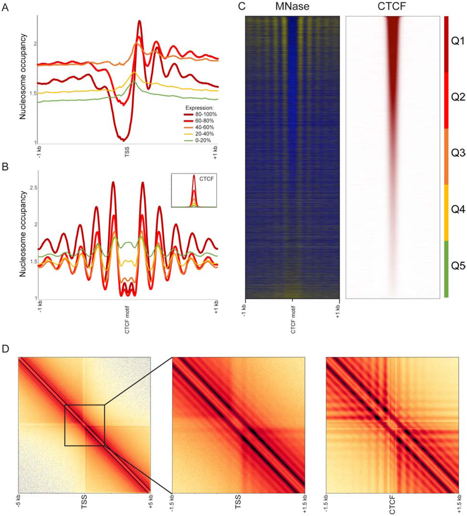
(A-C) Micro-C recovers nucleosome-resolution chromatin organization. In these panels, read pairing information was discarded, and single-end Micro-C reads (representing nucleosome ends) were shifted 73 bp to the nucleosome dyad axis. (A-B) show nucleosome occupancy profiles aligned according to TSSs (A) or CTCF binding sites (B) and averaged according to quintiles of transcription rate (using Pol2 occupancy as a proxy) or CTCF occupancy. Panel (C) shows nucleosome occupancy and CTCF ChIP enrichment (Davis et al., 2018) at CTCF binding sites sorted from high (top) to low (bottom) CTCF occupancy.

(D) Nucleosome resolution contact maps surrounding TSSs (left two panels) or CTCF binding sites (right panel). Promoters and CTCF sites act as boundaries between contact domains, as seen in the clearing of contacts in the upper right and lower left quadrants. Also apparent at this resolution is the nucleosome phasing surrounding these regulatory elements, manifest as a grid-like structure superimposed on the contact maps. See also Supplementary Figure S3A.

Including the information contained in the proximity ligations between nucleosomes allows us to use Micro-C to its full potential and capture local features of the chromatin fiber that are beyond the typical resolution of Hi-C. Given the key roles for CTCF and promoters in organizing local 1D chromatin, we started by exploring the local nucleosome-nucleosome interactions around TSSs and CTCF binding sites. Averaged read-level interaction maps centered at these elements (Figure 2D, Supplementary Figure S3A) produce a characteristic pattern of accumulation (“inverted egg-carton”), with two distinct banding patterns: (i) a series of horizontal/vertical bands decaying from the center, reflecting the coherent positioning of individual nucleosomes in the vicinity of a DNA-bound factor and (ii) a series of bands parallel to and decaying away from the main diagonal, reflecting a coherence in the interactions among neighboring nucleosomes throughout the fiber. Importantly, this diagonal banding is consistently observed at varying distances from regulatory elements (compare diagonal banding immediately downstream of TSSs vs. 5 kb away), providing a locus-resolved view of the genome-averaged oscillations seen in global interaction decay curves (Supplementary Figures S1E–G). This finding indicates that nucleosomes are generally organized into regularly spaced arrays genome-wide, regardless of how coherent the positioning of such arrays may be from cell to cell at any given locus. In other words, although, say, the +6 nucleosome in a coding region may exhibit “fuzzy” positioning in ensemble measurements, occupying different positions in different cells in a population, the adjacent nucleosomes are consistently well-positioned relative to this nucleosome.

To further explore local chromatin fiber behavior in our Micro-C maps, we focused on the behavior of interaction decay curves at short (1–10 nucleosome) distances (Supplementary Figure S1F–G). The behavior of the contact frequency decay at short distances allows us to discount a solenoid-like organization as we find no enrichment of N/N+5 or N/N+6 ligation products. In contrast, we find a subtle signature for a given nucleosome to interact with similar efficiency with adjacent pairs of distal nucleosomes (eg N+2 and N+3, or N+4 and N+5 – see Supplementary Figure S1G). Thus, our data support the emerging model that small (~3–10) “clutches” of nucleosomes are organized in a 2-start or zig-zag orientation to form short tri- or tetranucleosome zig-zag motif (Dorigo et al., 2004; Grigoryev et al., 2009; Hsieh et al., 2015; Ohno et al., 2019; Ou et al., 2017; Ricci et al., 2015; Risca et al., 2017; Song et al., 2014; Yao et al., 1993). Although the precise underlying structure of the chromatin fiber cannot be directly extrapolated from our data, the interaction decay curves provide strong experimental constraints to test theoretical models.

High resolution analysis of domain boundaries in Micro-C

Next, we turn to the organization of domains and boundaries in human cells. TADs are chromatin domains thought to emerge as the result of continuous ATP-dependent extrusion of chromatin loops by cohesin. Simulations have shown that the stopping of cohesin, e.g. by DNA-bound CTCF molecules, can create TAD boundaries, as well as other patterns of contact enrichment observed in Hi-C maps (Fudenberg et al., 2016; Sanborn et al., 2015). These signatures include 1) a square or box on the diagonal, with elevated contact frequencies within a square delimited by sharp boundaries (Dixon et al., 2012; Nora et al., 2012), 2) stripes along the box edges (Fudenberg et al., 2016), and 3) dots at their far corners (Rao et al., 2014). Stripes and dots are attributed to the stalling of extruded loops at one or two inward-oriented CTCF binding sites, respectively.

To leverage the enhanced resolution afforded by Micro-C to precisely identify genomic correlates of boundary activity (Figure 3A), we defined chromatin interaction boundaries by scanning the genome for local minima in the number of crossing interactions (normalized relative to the local interaction frequency at the same distance (Crane et al., 2015)), i.e. insulation strength. Boundary calls were robust to three different parameter choices (Supplementary Figure S3B). To identify genomic features associated with boundary activity, we sorted boundaries by their insulation strength and searched for previously-mapped factors (Davis et al., 2018) that were correlated with boundary activity (Figures 3B–D). Consistent with prior Hi-C analyses of domain folding (Dixon et al., 2012; Rao et al., 2014), we find architectural factors including RAD21, CTCF, YY1, and ZNF143 enriched at strong boundaries. More generally, boundaries are highly enriched for promoter marks and are localized precisely to nucleosome-depleted regulatory elements, consistent with the prior identification of TSSs as boundary elements in budding and fission yeast (Hsieh et al., 2015; Hsieh et al., 2016) and mouse cell lines (Bonev et al., 2017). Moreover, boundary behavior was correlated with promoter strength in both HFFs and ESCs (Supplementary Figures S3A,C), and this correlation was dynamic – promoters activated in HFFs exhibit stronger boundary activity in this cell type, and vice-versa (Supplementary Figure S3D).

Figure 3. High resolution identification of interaction boundaries.

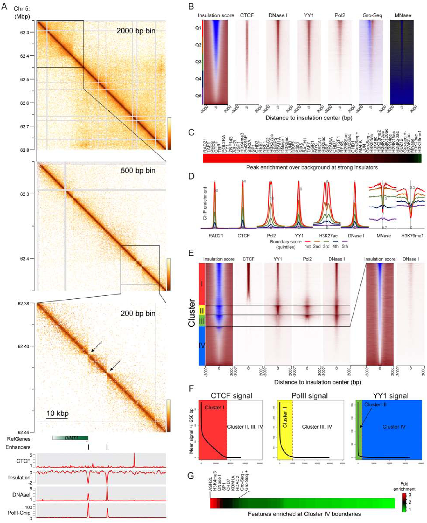
(A) Successive zooms into the ESC Micro-C dataset show a boundary between selfassociating domains, located at a promoter. Bottom panel shows genomic tracks for CTCF, insulation score, DNaseI signal, and Pol2 ChIP.

(B) Gross features of boundary elements in ESCs (all systematic comparisons are performed in ESCs given the abundant ChIP-Seq data available in this cell type). Boundaries were identified as described in Methods, and the strongest 100,000 boundaries are sorted according to insulation score (left panel). See also Supplementary Figure S3B. Right panels show ChIP-Seq enrichment for key boundary factors, DNase- and MNase-Seq data, and GRO-Seq as a readout of active transcription.

(C) Survey of factors enriched at strong boundaries. For the indicated ChIP-Seq (and DNase- and MNase- Seq) datasets, the peak to trough (ChIP signal at the central 500 bp vs. the baseline, 2 kb distant) ratio was calculated, and factors are ordered by enrichment score.

(D) Examples of boundary-enriched (CTCF, etc.) and -depleted (H3K79me2) factors.

(E-G) Independence of key boundary elements. Boundaries were successively sorted by CTCF, YY1, and Pol2 to group boundaries into four classes – CTCF-associated, CTCF-negative/Pol2-positive, CTCF/Pol2-depleted/YY1-positive, and weak CTCF/YY1/Pol2-depleted boundaries. Panel (E) shows heatmaps of relevant signals at the four boundary types, along with a zoom-in of insulation score and DNase I signal at Cluster IV boundaries. See Supplementary Figure S3F for more Cluster IV-associated features. Panel (F) shows the distribution of signal for CTCF, Pol2, and YY1 at all boundaries (left panel), CTCF-depleted boundaries (middle panel), and CTCF- and Pol2-depleted boundaries (right panel). For each distribution, the threshold for calling factor depletion is indicated as a dotted vertical line. (G) shows enrichment of a various proteins or other features at Cluster IV boundaries – full set of labels is provided in Supplementary Figure S3E.

Boundary activity at CTCF binding sites and at promoters is also readily apparent as clearing of interactions in the upper-right/lower-left corners of the CTCF- and TSSaligned heatmaps in Figure 2D. Importantly, although binding of CTCF and YY1 are both strongly positively-correlated with boundary scores (Figure 3B), these factors did not always co-occur at every boundary – Figures 3E–G show successive classification of boundaries into CTCF-associated boundaries, CTCF-negative YY1-enriched boundaries, CTCF- and YY1-depleted promoter boundaries, and a fourth class of weak boundaries largely depleted of all three features (Figure 3E, Supplementary Figures S3E–F). Overall, although multiple factors are associated with boundaries that separate contact domains from one another, the common feature of boundaries identified here was some le vel of nucleosome depletion, as exemplified by DNase I sensitivity.

Together, these data precisely localize chromatin domain boundaries in human cells, emphasizing the tight association between nucleosome depletion/dynamics (and/or the diverse set of proteins that occupy various nucleosome-depleted regions) as key players in insulating adjacent chromatin interaction domains from one another.

Identification of thousands of novel looping interactions in Micro-C maps

Among other TAD-associated structural features, we noted that the most apparent difference between Hi-C and Micro-C maps is a profusion of dots in Micro-C that are indistinct or absent in Hi-C maps (Figure 4A, Supplementary Figures S4A–B). This intuition is confirmed computationally, as systematic identification of looping interaction peaks (Methods) reveals a massive increase in the number of dots and dot anchor loci in Micro-C maps relative to Hi-C (Figure 4B). In general, the majority of dots detected in Hi-C libraries were also detected with Micro-C (86.6% in ESC, 89.4% in HFF), although even for these Hi-C/Micro-C common dots the Micro-C dataset exhibited increased signal over local background (Figure 4C, Supplementary Figure S4C). Conversely, averaging interaction maps for Micro-C-specific dots revealed a low level of signal enrichment at these locations in the Hi-C dataset (Figure 4C, Supplementary Figure S4C), indicating that evidence for these interaction peaks is present in both datasets but that Micro-C resolves more dots as a consequence of the improved signal-to-noise of this protocol.

Figure 4. TADs are composed of a heterogeneous network of internal looping interactions.

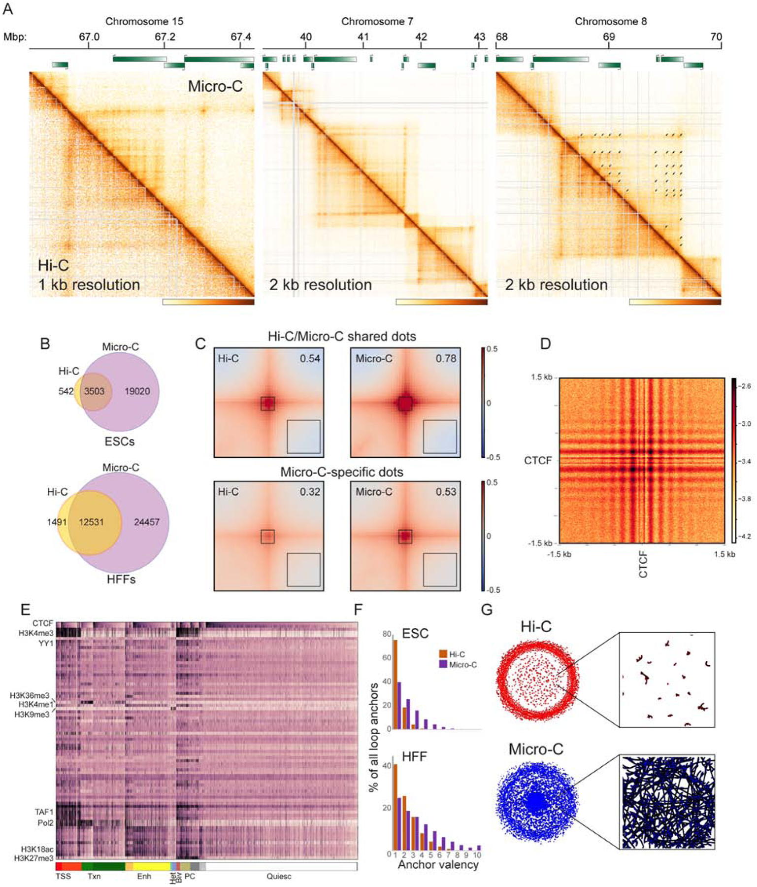
(A) Examples of Micro-C-specific peaks of looping interactions in HFFs. In each case Micro-C contact map is shown above the diagonal, along with corresponding Hi-C heatmap below the diagonal (see also Supplementary Figures S4A–B for ESC examples). Arrows in the right panel show “dots” called in the Micro-C dataset.

(B) Venn diagrams show presumed looping interaction peaks (dots) identified by MicroC and Hi-C in ESCs and HFFs, as indicated.

(C) Heatmaps showing average contact frequency in ESCs for dots called in both Hi-C and Micro-C (top), or in Micro-C only. Heatmaps show data for 200 kb (100 kb upstream and 100 kb downstream) surrounding loop anchors. Number in the upper right hand corner represents the signal strength at the loop base (heatmap center) over the nearby background (black box, lower right corner). See also Supplementary Figure S4C for HFF dataset.

(D) Heatmap showing average contact frequency, at nucleotide resolution, for all pairs of CTCF ChIP-Seq peaks associated with convergently-oriented CTCF motifs at separations between 100 kb and 1 Mb. See also Supplementary Figure S5.

(E) Global view of dot anchor sites. For all anchor sites, enrichment for various chromatin proteins or histone modifications (Davis et al., 2018) was computed. Anchor sites are first sorted according to chromatin state (broad chromatin types indicated at bottom, from left: Transcription Start Sites, Transcribed chromatin, Enhancers, Heterochromatin, Bivalent, Polycomb, and “Quiescent” chromatin depleted of characteristic proteins/modifications), then sorted according to CTCF enrichment within each subcluster. See also Supplementary Figures S6–7.

(F)Micro-C identifies genomic loci with multiple looping interaction peaks. Histograms show the number of looping interaction peaks for any given genomic locus, revealing a clear shift towards multiple peaks in Micro-C compared to Hi-C datasets.

(G)Grid completeness. Left panels show networks constructed from Hi-C (top) and Micro-C (bottom) looping interaction peaks, while right panels show a zoom in from the center of the network. Here, nodes represent genomic loci (anchors), while edges represent interaction peaks between anchor sites (dots).

Where are Micro-C-specific dots located? We noted that many examples of Micro-C dots were found along the extrusion-associated stripes at TAD borders (Figure 4A), suggesting the presence of multiple, relatively weak, pause sites that temporarily arrest SMC extrusion complexes before these complexes reach the “hard stop” boundaries previously observed at inwardly-oriented CTCF sites (Nora et al., 2017; Rao et al., 2014). Moreover, we often observed Micro-C-specific dots populating the interior of TAD boxes, located at intersections of the newly-identified weak pause sites found along TAD-bordering stripes. What is the nature of the newly-identified genomic dot anchors? Consistent with the central role for CTCF in blocking or pausing loop extrusion (Nora et al., 2017; Rao et al., 2014), we find that the majority of new dot anchors coincide with ChIP-Seq peaks of CTCF enrichment, with ~77% of all dot anchors linked to CTCF binding sites (Supplementary Figure S5A). To explore ultrastructural features of CTCF-anchored looping interactions, we produced read-level pileup contact maps averaging off-diagonal pairs of CTCF binding sites for both convergently-oriented binding sites (Figure 4D) as well as binding sites in tandem or divergent orientations (Supplementary Figures S5B–E). Two salient features of these heatmaps are worth noting. First, at high resolution, the beading of the central interactions reveals interactions between the well-positioned nucleosomes flanking CTCF binding sites. Second, the horizontal and vertical lines on these heatmaps are consistent with the stripes that characterize the loop extrusion process in Hi-C contact maps. Importantly, the extension of these stripes beyond (above or to the right of) the anchor points is consistent with many of these CTCF-mediated dots occurring in the middle of a loop extrusion track, generalizing our observation that many Micro-C-specific dots are identified along these extrusion stripes (see, e.g, Figures 1A and 4A).

To explore the molecular features of these enriched looping interactions, we calculated the enrichment of a variety of structural proteins and histone modifications at dot anchors, then clustered dot anchors according to these features (Figure 4E, Supplementary Figure S6A). We find that multiple classes of genomic loci are involved in looping interaction peaks, including: 1) Promoters (enrichment for H3K4me3, Pol2); 2) Enhancers (H3K4me1); 3) Coding regions (H3K36me3, Pol2); 4) Polycomb chromatin (H3K27me3, SUZ12); 5) “Quiescent” chromatin (depleted of distinguishing histone marks). Beyond the expected enrichment of CTCF at dot anchors, we identify a number of CTCF-depleted dot anchors (see examples in Supplementary Figures S4A–B), although interestingly these anchors were generally found at the same types of genomic element as the CTCF-enriched anchors (Supplementary Figures S6B–C). Given that systematic identification of dot anchors is somewhat inefficient – for instance, Micro-C-specific dots clearly exhibit modest signal in Hi-C but are not called – we further explored CTCF-independent dots by averaging interactions between various pairs of CTCF-depleted genomic loci (Supplementary Figure S7). These heatmaps reveal strong Micro-C signal enrichment for enhancer-promoter interactions (Supplementary Figures S4A–B, S7A), as well as dots occurring between paired binding sites for a wide array of transcriptional and chromatin regulatory proteins (Supplementary Figure S7B).

Finally, we noted that most of the new dots identified by Micro-C were relatively weak interaction peaks occurring either at the intersection points of new anchor sites in the interior of TADs, or along stripes associated with strong CTCF dots at TAD corners. This suggests that a given genomic locus can participate in multiple distinct, presumably transient, loops across a cell population. To more systematically evaluate these qualitative observations, we first plotted the number of dot interactions for each genomic location involved in at least one dot. Consistent with visual examination, we find a significant increase in the fraction of dot anchors that participate in more than one interaction in Micro-C, relative to Hi-C (Figure 4F). The implication of this finding is that Micro-C reveals a more extensively interconnected network among genomic loci. Indeed, visualization of connectivity networks derived from Hi-C and Micro-C data (Figure 4G) revealed a more densely connected structure for the Micro-C dataset. In graph theory terms, this can be quantitated as node transitivity (Harary and Kommel, 2010), with the Micro-C network exhibiting significantly greater transitivity than the Hi-C network (0.46 vs. 0.29 for ESCs, 0.57 vs 0.48 for HFFs), confirming that Micro-C dot interactions form a more complete grid than do Hi-C dots.

DISCUSSION

Continuing development of 3C-related methods will provide increasingly detailed insights into the 3-dimensional organization of the genome in a wide variety of biological contexts. Here, we show that Micro-C provides the highest resolution and signal-tonoise of any whole genome Hi-C protocol to date, illuminating several features of chromosomal organization with remarkable clarity. In effect, Micro-C reveals internal structures that are “blurred out” by noise and the coarser capture radius of restriction enzyme Hi-C.

Most notably, our data provide a dramatically expanded list of genomic loci involved in presumed looping interactions, identifying ~3–5-fold more looping interactions than observed with in-situ Hi-C maps. Overall, newly-identified loops share similar features to previously-identified genomic looping interactions – they are located at regulatory elements and strongly but not exclusively associated with CTCF binding – but many of these newly-identified loop anchors fall along loop extrusion tracks. These newly-identified looping interactions therefore imply the presence of multiple weak pause sites that slow or stall SMC movement. This finding suggests an updated view of TADs as heterogeneous populations made up of multiple transient loops formed as SMC extrusion complexes slow down as they pass these weak pause sites, before they are more stably arrested at previously-described strong loop anchors. At present, it is unclear what distinguishes CTCF-associated weak pauses from the stronger pause sites previously identified – although some of these CTCF-binding motifs are oriented “away” from the direction of loop extrusion, this cannot account for the multitude of weak pause sites often seen on the same extrusion flare (see for example the right panel of Figure 4A). It seems likely that CTCF binding is more dynamic or spans a shorter fraction of the cell cycle at weak pause sites than at hard stop sites, or that CTCF-associated proteins present only at a subset of CTCF binding sites play important roles in arresting cohesin.

Several other features of the chromatin landscape are appreciable with the improved resolution of the Micro-C protocol. For instance, we localize boundaries between contact domains precisely to nucleosome-depleted regions, consistent with the location of contact domain boundaries in yeast (Hsieh et al., 2015; Hsieh et al., 2016) and mouse (Bonev et al., 2017), and suggesting that multiple distinct factors can interfere with interactions between adjacent chromatin domains. In other words, not only do well-studied factors such as CTCF insulate chromatin domains from one another, but other molecular machines that are associated with nucleosome depletion at regulatory elements also drive chromatin domain insulation (either by virtue of their association, or as a result of nucleosome depletion itself). Finally, and most uniquely, Micro-C maps include a one-dimensional nucleosome occupancy/positioning map “for free” thanks to the use of MNase to fragment the genome. As nucleosome depletion is one of the defining characteristics of active regulatory elements, Micro-C comparisons of different cell states (different cell types, control vs. knockdown, etc.) therefore provides simultaneous insights into both chromosome folding as well as the overall regulatory landscape across the genome.

Taken together, our data provide a rich resource for further investigation of the 3-dimensional chromosome organization of two distinct human cell types. Our data also emphasize the improved signal-to-noise, as well as superior genomic resolution, of Micro-C relative to Hi-C. Micro-C can be readily adapted to a wide variety of biological contexts, where the improved resolution and concomitant nucleosome mapping dataset should provide novel insights into chromosome organization.

STAR METHODS

LEAD CONTACT AND MATERIALS AVAILABILITY

Further information and requests for resources and reagents should be directed to and will be fulfilled by the Lead Contact, Oliver Rando (oliver.rando@umassmed.edu). This study did not generate new unique reagents.

EXPERIMENTAL MODEL AND SUBJECT DETAILS

Cell lines and culture conditions

Human Embryonic stem cells (H1 – WiCell, WA01, lot # WB35186, male) were cultured in mTeSR1 media (StemCell Technologies, 85850) under feeder-free conditions on Matrigel hESC-qualified matrix (Corning, 354277, lot # 6011002) coated plates at 37°C and 5% CO₂. H1 cells were daily fed with fresh mTeSR1 media and passaged every 4–5 days using ReLeSR (StemCell Technologies, 05872) reagent. For collection, cells were dissociated in to single cells with TrypLE Express (Thermo Fischer Scientific, 12604013), washed once with 1X PBS, and then roughly 20 mio cells were resuspended in 1x PBS (1 mL per 1 mio cells) for crosslinking with 1% Formaldehyde for 10 min RT. Formaldehyde crosslinking was quenched with glycine (final concentration 125 mM) for 5 min at RT. After washing with 1x PBS, resuspended cells were further crosslinked with 3 mM DSG (Thermo Fischer Scientific, 20593) in PBS at 4 mio cells/ml for 40 min with rotation at RT. Crosslinking was quenched with 0.4 M glycine (final concentration) for 5 min at RT, washed with 1x PBS, and cells were flash frozen in aliquots of 5 mio cells.

For HFFs, HFFc6 cells (male) were cultured according to 4DN Standard Operating Procedures. Cells were grown at 37 °C under 5% CO₂ in 75cm2 flasks containing Dulbeco’s Modified Eagle Medium (DMEM), supplemented with 20% heat inactivated Fetal Bovine Serum (FBS). For sub-culture, cells were rinsed with 1x DPBS and detached using 0.05% trypsin at 37 °C for 2–3 minutes. Cells were typically split ever y 2–3 days at a 1:4 ratio and harvested while sub-confluent, ensuring they would not overgrow. HFFc6 were harvested at 70–80% confluency. Plates were washed 2x with Hank’s Buffered Salt Solution (HBSS), and cells were crosslinked on plate with 1% FA diluted in HBSS for 10 min at RT. Crosslinking was then quenched with 128 mM glycine at RT 5min, then on ice 15 min. Cells were scraped into 50 ml tubes and washed 2x with DPBS. Second round crosslinking was then performed with DSG at 3 mM final concentration at RT for 40min, quenched with 0.4 M glycine, washed 2X with 0.5% BSA in DPBS, and flash frozen in aliquots of 5 mio cells.

METHOD DETAILS

Generation of in-situ Hi-C libraries

Deep Hi-C libraries were prepared following the Hi-C 2.0 protocol as previously described (Belaghzal et al., 2017). Briefly, for each deep library, 4× 5 million cells were crosslinked with 1% formaldehyde for 10 minutes at room temperature. Cells were lysed and chromatin was digested overnight at 37°C with DpnII (NEB), In sit u ligation of was performed for 4 hours at 16°C with T4 DNA ligase (Invitrogen) on ends that were blunted in the presence of biotin-14dATP (Invitrogen). DNA was isolated after reverse crosslinking at 65°C with proteinase K (Sigma). Then, biotin was removed from unligated ends at 20°C for 4 h using T4 DNA polymerase (NEB) in the absence of dTTP and dCTP. DNA was fragmented to 200–300bp by Covaris sonication followed by a double size selection with SPRI beads (AMpure XP, Beckman Coulter) to select for DNA of 250–350bp. After end repair, biotin labeled DNA was pulled down by streptavidin coated MyOne C1 beads (Invitrogen) on a magnetic stand. Illumina paired-end sequencing adaptors were ligated to both ends at room temperature for 2 hours (T4 DNA ligase, Invitrogen) and PCR was performed using Pfu Ultra fusion DNA polymerase (Stratagene) to generate the final Hi-C library. Primers were removed with SPRI beads and 4 tubes were pooled prior to sequencing. Typically, deep libraries were generated from a minimum of 8 lanes of sequencing using our in-house Illumina Hi-seq 4000.

MicroC-XL

The Micro-C XL protocol was adapted from (Hsieh et al., 2016). Frozen cells were resuspended in 200 μl cold 1x PBS (10 mM Na2HPO4/KH2PO4, pH 7.4, 137 mM NaCl, 2.7 mM KCl,) per 1 mio cells and split into 1 mio cells aliquots. Note, 1x BSA (NEB, #B9000S) was added to PBS prior resuspension and wash to reduce stickiness of HFFc6 cells to the tub walls. After 20 min incubation on ice, cells were collected by centrifugation (5000x g, 5 min), washed with 500 μl buffer MB#1 (10 mM Tris-HCl, pH 7.5, 50 mM NaCl, 5 mM MgCl2, 1 mM CaCl2, 0.2% NP-40, 1x Roche cOmplete EDTA-free (Roche diagnostics, 04693132001)), collected by centrifugation (5000 g, 5 min), and resuspended in 200 μl MB#1. Chromatin was fragmented with MNase for 10 min at 37°C. MNase concentrations were chosen to yield mostly mono-nucleosomal fragments, as tested in prior digestion tests, typically 5–20 U MNase (Wortington Biochem, LS004798). The digestion was stopped by addition of 0.5 M EGTA (Bioworld, #405200081) to a 1.5 mM final concentration and incubation at 65°C f or 10 min.

Chromatin aliquots were pooled for further processing. Here, the equivalent of 2.5 mio cells input yielded the best results, more than 5 mio cell-equivalent per aliquot is not recommended. The chromatin was collected by centrifugation (5000x g, 5 min), washed with 500 μl 1x NEBuffer 2.1 (NEB, #B7202S), collected by centrifugation (5000x g, 5 min), and resuspended in 45 μl NEBuffer 2.1. DNA ends were dephosphorylated by addition of 5 μl rSAP (NEB, #M0203) and incubation at 37°C for 45 min. The reaction was stopped by incubation at 65°C for 5 min. 5’ overhangs were generated by 3’ r esection. Here, 40 μl pre-mix (5 μl 10x NEBuffer 2.1, 2 μl 100 mM ATP (Thermo Fisher, #R0441), 3 μl 100 mM DTT, 30 μl H2O) and 8 μl Large Klenow Fragment (NEB, #M0210L) and 2 μl T4 PNK (NEB, #M0201L) were added to the sample in respective order. The reaction was incubated at 37°C for 15 min. The DNA overhangs were filled with biotinylated nucleotides by addition of 100 μl pre-mix (25 μl 0.4 mM Biotin-dATP (Invitrogen, #19524016), 25 μl 0.4 mM Biotin-dCTP (Invitrogen, #19518018), 2 μl 10 mM dGTP and 10 mM dTTP (stock solutions: NEB, #N0446), 10 μl 10x T4 DNA Ligase Reaction Buffer (NEB #B0202S), 0.5 μl 200x BSA (NEB, #B9000S), 38.5 μl H2O) and incubation at 25°C for 45 min. The reaction was sto pped by addition of 12 μl 0.5 M EDTA (Invitrogen, #15575038) and incubation at 65°C for 20 min.

The chromatin was collected by centrifugation (10000x g), washed in 500 μl 1x Ligase Reaction Buffer, and collected by centrifugation (10000x g). The chromatin pellet was resuspended in 2500 μl ligation reaction buffer (1x NEB Ligase buffer, 1x NEB BSA, 12500 U NEB T4 Ligase (NEB, #M0202L)) and incubated rotating at RT for 2.5–3 h. After proximity ligation, the chromatin was collected, resuspended in 200 μl 1x NEBuffer 1 (NEB, #B7001S) and 200 U NEB Exonuclease III (NEB, #M0206S), and incubated for 5 min at 37°C to remove biotin from unligated ends. For deproteination and reverse crosslinking, 25 μl ProteinaseK (25mg/ml in TE with 50% glycerol) and 25 μl 10% SDS (Invitrogen, #15553–035) were added and the sample was incubated at 65°C o/n.

The DNA was first phenol/chloroform purified and second purified with DNA Clean & Concentrator Kit (Zymo, #D4013). The 300 bp sized MicroC library was purified via 1.5% agarose gel electrophoresis and extracted with Zymoclean Gel DNA Recovery Kit (Zymo Research, #D4002) with a final elution volume of 50 μl.

5 μl DynabeadsTM MyOneTM Streptavidin C1 beads (Invitrogen, #65001) were washed twice with 300 μl 1x TBW (5 mM Tris-HCl, pH 7.5, 0.5 mM EDTA, 1 M NaCl) and suspended in 150 μl 2x TBW (10 mM Tris-HCl, pH 7.5, 1 mM EDTA, 2 M NaCl). 100 μl H2O and 150 μl washed Streptavidin beads in 2x TBW were added to the sample and incubated rotation at RT for 20 min. The beads were washed twice with 300 μl 1x TBW and resuspended in 50 μl TE buffer. Sequencing libraries were prepared with NEBNext® Ultra™ II DNA Library Prep Kit for Illumina® (NEB, #E7645) according to protocol, except for the DNA purification and size selection prior PCR. Here, adaptor-ligated DNA was pulled-down via still attached Streptavidin beads and washed twice with 300 μl 1x TBW and once with 0.1x TE. Finally, the beads were resuspended in 20 μl 0.1x TE. PCR amplification, sample indexing, and DNA purification after PCR was performed with according to (NEB, #E7645) using NEBNext® Multiplex Oligos for Illumina®. The samples were sequenced on an Illumina HiSeq 4000 on 50 base pair paired end mode.

QUANTIFICATION AND STATISTICAL ANALYSIS

Chromosome Conformation Capture data processing

Hi-C and Micro-C datasets were processed with the distiller pipeline (https://github.com/mirnylab/distiller-nf). Briefly, reads were mapped to the human reference assembly hg38 using bwa mem with flags -SP. Alignments were parsed and pairs were classified using the pairtools package (https://github.com/mirnylab/pairtools) to generate 4DNcompliant pairs files. Pairs having matching alignment strands and coordinates with a possible 1 bp offset were considered PCR and/or optical duplicates and thus removed.

Pairs classified as uniquely mapped or rescued chimeras with high mapping quality scores on both sides (MAPQ > 30) were aggregated into contact matrices in the cooler format using the cooler package (https://www.biorxiv.org/content/10.1101/557660v1) at 500bp and into multiresolution cooler files (500bp, 1kb, 2kb, 5kb, 10kb, 50kb, 100kb, 250kb, 500kb, 1Mb). All contact matrices were normalized using the iterative correction procedure (Imakaev et al., 2012) after bin-level filtering. Low-coverage bins were excluded using the MADmax (maximum allowed median absolute deviation) filter on genomic coverage, described in (Schwarzer et al., 2017), using a threshold of 5.0 MADs. To remove short-range ligation artifacts at a given resolution— such as unligated and self-ligated molecules—we removed pairs mapping to the same or adjacent genomic bins.

Contact heatmaps

The dense matrix data was extracted from balanced cooler files with cooltools package in python and plotted with gridGraphics package in R. The maximum color intensity was set to the percentile that allowed the best assessment of matrix specific features, such as TADs or dots. For heatmaps that display MicroC and HiC within one heatmap, the value-to-color conversion was applied to the individual data sets for equal percentiles.

Eigenvectors

Compartmentalization was assessed using an eigenvector decomposition procedure based on (Imakaev et al., 2012), as implemented in the cooltools package (https://github.com/mirnylab/cooltools). Eigenvector decomposition was performed on observedover-expected cis contact maps at 100-kb resolution, separately for each chromosomal arm, after subtracting 1. The first three eigenvectors and eigenvalues were calculated, and the eigenvector associated with the largest absolute eigenvalue was chosen. We used an identically binned track of gene frequency to orient the eigenvectors such that the positive and negative values of the eigenvector correlate with high and low gene density, respectively.

Interaction decay

Scaling curves of contact frequency as a function of genomic separation were generated by aggregating normalized contact frequency over valid pixels along diagonals of 1kb-resolution cis contact maps, with diagonals grouped into geometrically increasing spans of genomic separation. Scaling curves were also generated for unbinned data (uniquely mapped paired-end reads) using a similar methodology, independently for reads having each of four possible strand orientations. Average contact frequency P(s) curves are displayed using log-log axes.

Scaling curves of contact frequency as a function of genomic separation for short distances were generated from valid pairs files. Here, the distance between the read starts of uniquely mapped, cis reads were extracted and normalized for a distance of 1 to 100 kb to 1. For read shifted interaction decay curves, the read starts were shifted by 73 bp with respect to read orientations.

When controlling for number of reads (Supplementary Figure S1C), the data was subsampled using binomial subsampling of data binned at 1kb such that the total number of cis reads were the same between Hi-C and Micro-C following which, the interaction decay curves were generated.

Normalization at large distances (Supplementary Figure S1D) was done using iterative correction (Imakaev et al., 2012) that ignored reads at distances less than 10kb. This allowed us to normalize reads at large distances without explicitly removing short distance reads.

Insulation score

Diamond insulation scores (Crane et al., 2015) were calculated on 1-kb resolution maps using the cooltools package. A local minima detection procedure based on peak prominence, described in (Nora et al., 2017) and implemented in cooltools, was used to call insulating loci.

The diamond insulation (Crane et al., 2015) was computed for 100 and 200 bp resolutions. Here, 100 bp and 200 bp binned, balanced multi-cooler files were generated form valid pairs files with reads shifted by 73 bp to the theoretical nucleosome dyad. The insulation score was computed with the cooltools insulation tool at 100 bp resolution with 1,000 and 10,000 bp diamonds and for a 200 bp resolution with a 2,000 bp diamond. The positions for the strongest 100,000 boundaries was extracted as alignment point for 1D analyses.

1D analysis

Genomic alignment points: The positions for the strongest 100,000 boundaries, transcription start site, or CTCF peak positions, were used as alignment points for 1D analysis.

Signal tracks: For nucleosome occupancy data, the first read of the Micro-C read pairs was mapped with Bowtie2 (2.3.2) and Samtools (1.4.1) against the human genome (hg38) using the following parameters (bowtie2 -p 16 --local -x {hg38 bowtie2 genome} -U {fastq.file} | samtools view -bS -o {output.bam} -) 2>&1 | tee {report.file}). To compute the nucleosome dyad density, the resulting read starts were shifted by 73 bp (strand sensitive) to obtain the theoretical nucleosome dyad. ChIP-seq signal data tracts were downloaded from ENCODE (see Table S2). Raw Gro-Seq data was downloaded from and processed as described in (Sigova et al., 2013).

Sorting of 1D heatmaps and computation of quintiles: The mean PolII ChIP-seq signal in a window form –150 to 250 bp around TSSs was computed with respect to the direction of transcription, was used as a proxy for transcription rate. For CTCF binding strength, the mean CTCF ChIP-seq signal around CTCF peaks (ENCFF368LWM) was computed in a window of – 100 to 100 bp. Similarly, the mean insulation score within a window of –100 to 100 bp at boundary sites was used to sort alignments at boundaries. Alignment sites with NA scores within a window of −100 to 100 bp around the alignment point were removed from analysis, as they represent unmappable regions within the genome. Quintiles were computed by extracting 5 equally sized lists of alignment points from sorted data.

Plotting of 1D heatmaps and average signal plots: The signal around alignment points for given samples were extracted within a −2000 to 2000 bp window. Windows with low signal in MNase single-end read datasets or NA values in insulation scores were removed as they represent unmappable regions. The extracted data was mean-binned for 25 bp bins and visualized with gridGraphics package in R. For average signal plots, the data was prepared as for heatmaps, but the mean signal for 25 bp bins was computed for given quantiles and plotted.

Contact frequency pileup maps

We used cooltools to calculate aggregate contact frequency maps (pileup maps) centered at specific genomic loci. For lists of single or paired genomic landmarks, pileup maps consist of aggregated contact map “snippets” encompassing fixed-length genomic windows along each axis, centered at the midpoints of the respective features. These snippets are extracted from either iteratively-corrected or observed-over-expected contact matrices or from unbinned contacts. For unbinned data, the coordinates of the 5’ ends of the alignments from each uniquely mapped molecule were shifted 73 bp along the alignment reference strand (i.e. to the approximate locations of the nucleosome dyad axes) before aggregating.

Due to the localization uncertainty associated with dot calls, which were performed on 5- and 10-kb contact maps, the pileup maps for those features were generated using 5-kb contact maps. For more precise genomic landmarks, pileup maps were generated using 500bp resolution contact maps. The pileup maps generated from unbinned data (paired-end reads) were centered on motifs associated with CTCF binding sites. This list of sites was created by intersecting CTCF ChIP-seq peaks from ENCODE (ENCFF368LWM) with a list of CTCF motifs (JASPAR motif ID #MA0139.1) using bedtools (Quinlan and Hall, 2010). The TSS pileup maps generated from unbinned data (paired-end reads), were centered around CAGE-seq peaks taken from ENCODE (ENCFF038OTF). CAGE-seq peaks were selected that were more than 5kb from CTCF ChIP-seq peaks to prevent contamination of nucleosome positioning due to CTCF close to genes.

Differential Expression Analysis

RNA-seq for HFFc6 was generated as part of the 4DN Consortium and RNA-seq from h1-ESC was obtained from ENCODE (ENCSR000COU). Both sets of fastq files were mapped using Bowtie2 (Langmead and Salzberg, 2012) and counts associated with genes were generated using RSEM (Li and Dewey, 2011) using default parameters. Finally, the edgeR package (Robinson et al., 2010) was used to do differential expression analysis. The resulting volcano plot was colored by changes in associated eigenvector value to generate Supplementary Figure S2C.

The average insulation score for promotors was computed as the average of 5× 100 bp bins from the 100 bp insulation vector with the last bin containing the TSS (sensitive to gene directionality). For Supplementary Figure S3C, genes were grouped by transcription rate into quintiles and the average insulation score at promoters was plotted. For Supplementary Figure S3D, genes with a 2-fold change of transcription rate between HFF and ESC cells were selected and the insulation score for ESC over HFF was plotted. Genes that were at least 2-fold down regulated in HFF compared to ESC were colored blue, genes that were at least 2-fold up regulated were colored red.

Dot detection

We reimplemented the HiCCUPS algorithm (Rao et al., 2014) in the form of the call-dots command line tool as a part of the cooltools package of tools for Hi-C data analysis (https://github.com/mirnylab/cooltools). This tool was used to identify locally enriched interactions, i.e. “dots”, both for Hi-C and Micro-C binned data. Dots were called at 5kb and 10kb resolutions using only high quality mapped pairs (MAPQ > 30) and the resulting lists were merged using the same criteria as in (Rao et al., 2014):

• matching dot calls were identified between 5kb and 10kb lists, assuming dots with Euclidian distance between them lower than 10kb as matching

• all unique dots called at 10kb were retained in the merged list

• only higher resolution, 5kb, dot-calls were retained, for the matching 5kb and 10kb calls - unique dot-calls at 5kb were retained only in case they were small (<100kb) in size, or particularly strong (>=100 raw interactions per 5kb pixel)

A detailed description of the dot calling procedure for a given resolution is provided in (Rao et al., 2014); here we briefly highlight some of the major steps and the deviations from the original procedure (Rao et al., 2014) that we assumed here:

• detecting locally enriched interactions, i.e. dot-calling, starts with defining locally-adjusted expected level of interactions for pixels on a heatmap

• in this case, we limit ourselves to survey only pixels that are separated by less than 10Mb, i.e. 10Mb-wide band near the diagonal on the heatmap was surveyed.

• for a given pixel, its locally-adjusted expected defined as the average distance decay corrected by the enrichment of the area surrounding the pixel of interest, i.e. P(s)*donut_observed/donut_expected

• like in HiCCUPS, we employ 4 independent filter-shapes: “donut”, low-left, vertical, and horizontal

• our calculation of local enrichment factor deviates from the original HiCCUPS - we do not adjust the footprint of the filters neither for pixels near the diagonal nor for pixels in sparse areas of the heatmap, instead we convolve a fixed size filters/kernels with the observed/expected heatmaps to calculate local enrichment factors

• surveyed pixels are grouped into so-called lambda-chunks according to their level of locally-adjusted expected and BH-FDR is performed for each of lambda-chunks independently, as described in (Rao et al., 2014).

• pixels identified as significant in each lambda-chunk constitute the filtered list of peak calls that gets post-processed the same way as in the original HiCCUPS procedure

• clustering is done using Birch initialization procedure and additional enrichment thresholding is performed along with the special treatment of the non-clustered singletons.

Dot anchor analysis

Dot calls between Hi-C and Micro-C were compared using the following methodology. First, for each individual list of dot calls (Hi-C and Micro-C), every call was assigned a unique protocol-specific dot-call ID. Then, the left (5’-most) anchor intervals from the two call lists were intersected using bedtools intersect, such that every resulting intersection was associated with a pair of dot-call IDs (one from each protocol). The same procedure was applied to intersect the right (3’-most) anchor intervals from the two call lists. Common dots were identified from matching pairs of dot-call IDs found in the two intersection sets. The remaining dot calls were identified as unique to their respective protocol of origin. To account for uncertainty in dot localization, we increased the genomic extent of each dot anchor interval by 10kb in each direction before performing the intersections.

Distinct anchor regions from dot calls were assessed using a similar methodology. First, for each protocol, overlapping anchor intervals across all dot calls were grouped using bedtools cluster with -d 20000 and those groups were merged to produce a list of non-overlapping consensus intervals. The consensus anchor interval lists from Hi-C and Micro-C were then combined and the intervals grouped using the same command. The groups were then merged to produce a final consolidated list of non-overlapping anchor intervals. Those final anchor intervals derived from only one of the two protocols were identified as being unique to that protocol, while the remaining consolidated intervals were identified as being common to both protocols.

Dot anchor graph analysis

Networks were constructed using lists of dots, where dot anchors represent nodes while dot calls represent edges between nodes. Such a representation allows us to leverage the properties of networks for the comparison of the lists obtained from the two protocols. Specifically, we look at the degree distribution and clustering coefficient of the network.

The degree distribution of the network represents the distribution anchor valencies. The network is constructed, and the degree of each node is extracted. A histogram of the degrees can be generated for each network and compared.

The clustering coefficient is a frequently used property of networks that measures the average interconnected-ness of the local neighborhood of around nodes. The clustering coefficient is calculated as the 3 times the ratio of closed triangles to open paths of length 2 found in the network. A fully connected graph would have a coefficient of 1. For the network of dots calls, distance dependence of dots ensures that its network will never be fully connected. To account for this, we adjust the transitivity by dividing it by the transitivity of a network that is fully connected up to 2 Mb generated from all the anchors associated with the dots.

CTCF occupancy of dot anchors

Dot anchors were intersected with CTCF ChIP-seq peaks using bedtools intersect. Since the genomic regions associated with dot anchors were extended during the clustering and accumulation process, no additional margins were introduced when intersecting with CTCF peaks.

For both classes of dot anchors (with a CTCF peak and without a CTCF peak), the mean fold change of CTCF ChIP-seq over the anchor region was also calculated and recorded and histograms were constructed.

Epigenetic characterization of ESC dot anchors

Each distinct dot anchor interval identified in H1 hESCs was classified by its modal ChromHMM state assignment from the Epigenomics Roadmap 18-state model (trained on six core histone marks, 200bp bins) (Roadmap Epigenomics et al., 2015). Anchor intervals were further characterized by calculating the mean ChIP-seq signal in 10 kb windows around their midpoint for 79 histone and transcription factor experiments on H1 cells obtained from the ENCODE data portal (Table S3). These feature vectors were concatenated into a heatmap, where each row corresponds to a dot anchor. Columns of the heatmap were sorted based on Ward agglomerative clustering (n=6) and rows were grouped by ChromHMM state. Clustering the rows using K-means or agglomerative clustering produced similar epigenetic classifications of the dot anchors.

Loop analysis at E-P and CTCF-depleted loci

Enhancer locations for hg19 were downloaded from (http://zlab-annotations.umassmed.edu/enhancers/) and converted to hg38 with UCSC lift over tool (https://genome.ucsc.edu/cgi-bin/hgLiftOver). Intersections were computed with bedtools window –w 100000 function and intersections with distances smaller than 5 kb were removed.

Processed ChIP-seq peaks for chromatin binding factors were extracted from ENCODE (Table S4). ChIP-seq peaks that are within 10 kb of a CTCF peak were removed with bedtools window –w 10000 –v function. Intersections of ChIP seq peaks within a ChIP seq data set were generated with bedtools window –w 100000 function. Sites where the two intersection resulting anchors were closer than 5 kb were removed.

As above, aggregate contacts were extracted with cooltools snippets function observedover-expected contact matrices.

DATA AND CODE AVAILABILITY

Raw and processed files are available in the 4DN data portal (https://data.4dnucleome.org/ under the accession numbers 4DNESWST3UBH, 4DNES21D8SP8, 4DNES2R6PUEK, 4DNESRJ8KV4Q).

Supplementary Material

3

Table S1. Dataset overview, related to Figures 1–4.

Read count sheet shows read numbers for Hi-C and Micro-C libraries for ESCs and HFFs, as indicated. Rows indicate total read counts, mappable reads, and read pairs present on the same chromosome (cis) and those bridging chromosomes (trans). Replicate_IDs sheet shows biological and technical replicate numbers, along with 4DN (https://data.4dnucleome.org/) identification data.

4

Table S2. Public ChIP-Seq signal datasets used for comparisons to Micro-C 1D heatmaps and composite plots, related to Figure 3 and Supplementary Figure S3.

Publicly-available datasets used for analyses in Figure 3 and Supplementary Figure S3.

5

Table S3. Public ChIP-Seq datasets used for epigenetic characterization of ESC dot anchors, related to Figure 4 and Supplementary Figure S6.

As in Table S2, with datasets used for analyses in Figure 4 and Supplementary Figure S6.

6

Table S4. Public ChIP-Seq peak position datasets used for looping interaction pile-ups at CTCF-depleted loci, related to Figure 4 and Supplementary Figure S7.

As in Tables S2–3, with datasets used for analyses in Figure 4 and Supplementary Figure S7.

KEY RESOURCES TABLE

REAGENT or RESOURCE	SOURCE	IDENTIFIER
Chemicals, Peptides, and Recombinant Proteins
mTeSR1 media	StemCell Technologies	85850
Matrigel hESC-qualified matrix	Corning	354277
ReLeSR	StemCell Technologies	05872
TrypLE Express	Thermo Fischer Scientific	12604013
DSG	Thermo Fischer Scientific	20593
Dulbeco’s Modified Eagle Medium	Thermo Fisher Scientific DMEM-GlutaMax	10569010
Fetal Bovine Serum	VWR	97068–091
Hank’s Buffered Salt Solution	Thermo Fisher Scientific	14025092
T4 DNA ligase	Invitrogen	15224017
DpnII	NEB	R0543S
T4 DNA polymerase	NEB	M0203S
PfuUltra II Fusion High-fidelity DNA Polymerase	Agilent	600674
T4 DNA ligase	NEB	M0202S
proteinase K	Sigma	P2308–100MG
AMpure XP	Beckman Coulter	A63881
MyOne C1	Invitrogen	#65001
Q5 polymerase	NEB	M0491S
BSA	NEB	#B9000S
cOmplete EDTA-free	Roche diagnostics	04693132001
MNase	Wortington Biochem	LS004798
EGTA	Bioworld	#405200081
NEBuffer 2.1	NEB	#B7202S
rSAP	NEB	#M0203
ATP	Thermo Fisher	#R0441
Large Klenow Fragment	NEB	#M0210L
T4 PNK	NEB	#M0201L
Biotin-dATP	Invitrogen	#19524016
Biotin-dCTP	Invitrogen	#19518018
dNTP stock solutions	NEB	#N0446
T4 DNA Ligase Reaction Buffer	NEB	#B0202S
BSA	NEB	#B9000S
EDTA	Invitrogen	#15575038
T4 Ligase	NEB	#M0202L
NEBuffer 1	NEB	#B7001S
Exonuclease III	NEB	#M0206S
SDS	Invitrogen	#15553–035
Critical Commercial Assays
DNA Clean & Concentrator Kit	Zymo	#D4013
NEBNext® Ultra™ II DNA Library Prep Kit for Illumina®	NEB	#E7645
NEBNext® Multiplex Oligos for Illumina®	NEB	E7335S
Deposited Data
DpnII HiC - H1-ESC	This Study	https://data.4dnucleome.org/ (4DNESRJ8KV4Q)
Micro-C - HFFc6	This Study	https://data.4dnucleome.org/ (4DNESWST3UBH)
Micro-C - H1-ESC	This Study	https://data.4dnucleome.org/ (4DNES21D8SP8)
DpnII HiC - HFFc6	This Study	https://data.4dnucleome.org/ (4DNES2R6PUEK)
CAGE-seq peaks	ENCODE	ENCFF038OTF
HFFc6	4DN data portal	4DNESFH3EHTU
h1-ESC RNA-seq	ENCODE	ENCSR000COU
Gro-Seq	Sigova et al., 2013	N/A
for published genome-wide datasets see Tables S2–S4	N/A	N/A
Experimental Models: Cell Lines
HFFc6 (Tier 1)	4DN (https://www.4dnucleome.org/)	4DNSRC6ZVYVP
H1-hESC (Tier 1)	4DN (https://www.4dnucleome.org/)	4DNSRV3SKQ8M
Software and Algorithms
distiller	https://github.com/mirnylab/distiller-nf	v0.3.1
pairtools	https://github.com/mirnylab/pairtools	v0.2.1
cooler	https://www.biorxiv.org/content/10.1101/557660v1	v0.8.11
cooltools	https://github.com/mirnylab/cooltools	v0.1.0
Bowtie2	http://bowtie-bio.sourceforge.net/bowtie2/index.shtml	v2.3.2
Samtools	http://www.htslib.org/	v1.4.1
bedtools	https://bedtools.readthedocs.io/en/latest/	v2.27.1
RSEM	https://deweylab.github.io/RSEM/	v1.3.2
R	https://www.r-project.org/	v3.6.2
RColorBrewer	R package	v1.1–2
data.table	R package	v1.12.8
gridGraphics	R package	v0.4–1
zoo	R package	v1.8–7
HiGlass	https://higlass.io	v1.8
higlass-python	Python package	v0.1–0.4
pybbi	Python package	v0.2
numpy	Python package	v1.16–1.18
scipy	Python package	v1.2–1.4
matplotlib	Python package	v3.0–3.1
pandas	Python package	v0.24–1.0
scikit-learn	Python package	v0.20–0.22
h5py	Python package	v2.9–2.10
pyarrow	Python Package	v0.12–0.16
jupyter-notebook	Python package	v5.7–6.0
networkx	Python package	v2.2
edgeR	R package	N/A
nextflow	https://www.nextflow.io/docs/latest/index.html	v19.01.0
Singularity	https://www.nextflow.io/docs/latest/singularity.html	v3.0.3
Snakemake	https://snakemake.readthedocs.io/en/stable/	v5.2.2

Highlights.

1. Micro-C provides nucleosome resolution maps of chromosome folding

2. The resolution and signal to noise are significantly improved relative to Hi-C

3. Thousands of new loops are identified suggesting weak pauses to loop extrusion

4. New loops suggest TADs represent heterogeneous collections of transient loops

REFERENCES

- Beagrie RA, Scialdone A, Schueler M, Kraemer DC, Chotalia M, Xie SQ, Barbieri M, de Santiago I, Lavitas LM, Branco MR, et al. (2017). Complex multi-enhancer contacts captured by genome architecture mapping. Nature 543, 519–524. [DOI] [PMC free article] [PubMed] [Google Scholar]
- Belaghzal H, Dekker J, and Gibcus JH (2017). Hi-C 2.0: An optimized Hi-C procedure for high-resolution genome-wide mapping of chromosome conformation. Methods 123, 56–65. [DOI] [PMC free article] [PubMed] [Google Scholar]
- Boettiger AN, Bintu B, Moffitt JR, Wang S, Beliveau BJ, Fudenberg G, Imakaev M, Mirny LA, Wu CT, and Zhuang X (2016). Super-resolution imaging reveals distinct chromatin folding for different epigenetic states. Nature 529, 418–422. [DOI] [PMC free article] [PubMed] [Google Scholar]
- Bonev B, Mendelson Cohen N, Szabo Q, Fritsch L, Papadopoulos GL, Lubling Y, Xu X, Lv X, Hugnot JP, Tanay A, et al. (2017). Multiscale 3D Genome Rewiring during Mouse Neural Development. Cell 171, 557–572 e524. [DOI] [PMC free article] [PubMed] [Google Scholar]
- Carone BR, Hung JH, Hainer SJ, Chou MT, Carone DM, Weng Z, Fazzio TG, and Rando OJ (2014). High-resolution mapping of chromatin packaging in mouse embryonic stem cells and sperm. Developmental cell 30, 11–22. [DOI] [PMC free article] [PubMed] [Google Scholar]
- Crane E, Bian Q, McCord RP, Lajoie BR, Wheeler BS, Ralston EJ, Uzawa S, Dekker J, and Meyer BJ (2015). Condensin-driven remodelling of X chromosome topology during dosage compensation. Nature 523, 240–244. [DOI] [PMC free article] [PubMed] [Google Scholar]
- Cremer T, and Cremer M (2010). Chromosome territories. Cold Spring Harbor perspectives in biology 2, a003889. [DOI] [PMC free article] [PubMed] [Google Scholar]
- Davis CA, Hitz BC, Sloan CA, Chan ET, Davidson JM, Gabdank I, Hilton JA, Jain K, Baymuradov UK, Narayanan AK, et al. (2018). The Encyclopedia of DNA elements (ENCODE): data portal update. Nucleic acids research 46, D794–D801. [DOI] [PMC free article] [PubMed] [Google Scholar]
- Dekker J, Rippe K, Dekker M, and Kleckner N (2002). Capturing chromosome conformation. Science (New York, N.Y 295, 1306–1311. [DOI] [PubMed] [Google Scholar]
- Dixon JR, Selvaraj S, Yue F, Kim A, Li Y, Shen Y, Hu M, Liu JS, and Ren B (2012). Topological domains in mammalian genomes identified by analysis of chromatin interactions. Nature 485, 376–380. [DOI] [PMC free article] [PubMed] [Google Scholar]
- Dorigo B, Schalch T, Kulangara A, Duda S, Schroeder RR, and Richmond TJ (2004). Nucleosome arrays reveal the two-start organization of the chromatin fiber. Science (New York, N.Y 306, 1571–1573. [DOI] [PubMed] [Google Scholar]
- Falk M, Feodorova Y, Naumova N, Imakaev M, Lajoie BR, Leonhardt H, Joffe B, Dekker J, Fudenberg G, Solovei I, et al. (2019). Heterochromatin drives compartmentalization of inverted and conventional nuclei. Nature 570, 395–399. [DOI] [PMC free article] [PubMed] [Google Scholar]
- Finn EH, Pegoraro G, Brandao HB, Valton AL, Oomen ME, Dekker J, Mirny L, and Misteli T (2019). Extensive Heterogeneity and Intrinsic Variation in Spatial Genome Organization. Cell 176, 15021515 e1510. [DOI] [PMC free article] [PubMed] [Google Scholar]
- Friedman N, and Rando OJ (2015). Epigenomics and the structure of the living genome. Genome research 25, 1482–1490. [DOI] [PMC free article] [PubMed] [Google Scholar]
- Fu Y, Sinha M, Peterson CL, and Weng Z (2008). The insulator binding protein CTCF positions 20 nucleosomes around its binding sites across the human genome. PLoS genetics 4, e1000138. [DOI] [PMC free article] [PubMed] [Google Scholar]
- Fudenberg G, Abdennur N, Imakaev M, Goloborodko A, and Mirny LA (2017). Emerging Evidence of Chromosome Folding by Loop Extrusion. Cold Spring Harb Symp Quant Biol 82, 45–55. [DOI] [PMC free article] [PubMed] [Google Scholar]
- Fudenberg G, Imakaev M, Lu C, Goloborodko A, Abdennur N, and Mirny LA (2016). Formation of Chromosomal Domains by Loop Extrusion. Cell reports 15, 2038–2049. [DOI] [PMC free article] [PubMed] [Google Scholar]
- Grigoryev SA, Arya G, Correll S, Woodcock CL, and Schlick T (2009). Evidence for heteromorphic chromatin fibers from analysis of nucleosome interactions. Proceedings of the National Academy of Sciences of the United States of America 106, 13317–13322. [DOI] [PMC free article] [PubMed] [Google Scholar]
- Harary F, and Kommel HJ (2010). Matrix measures for transitivity and balance. The Journal of Mathematical Sociology 6, 199–210. [Google Scholar]
- Hsieh TH, Weiner A, Lajoie B, Dekker J, Friedman N, and Rando OJ (2015). Mapping Nucleosome Resolution Chromosome Folding in Yeast by Micro-C. Cell 162, 108–119. [DOI] [PMC free article] [PubMed] [Google Scholar]
- Hsieh TS, Fudenberg G, Goloborodko A, and Rando OJ (2016). Micro-C XL: assaying chromosome conformation from the nucleosome to the entire genome. Nature methods. [DOI] [PubMed] [Google Scholar]
- Hughes AL, and Rando OJ (2014). Mechanisms Underlying Nucleosome Positioning in vivo. Annual review of biophysics. [DOI] [PubMed] [Google Scholar]
- Imakaev M, Fudenberg G, McCord RP, Naumova N, Goloborodko A, Lajoie BR, Dekker J, and Mirny LA (2012). Iterative correction of Hi-C data reveals hallmarks of chromosome organization. Nature methods 9, 999–1003. [DOI] [PMC free article] [PubMed] [Google Scholar]
- Lai WKM, and Pugh BF (2017). Understanding nucleosome dynamics and their links to gene expression and DNA replication. Nature reviews. Molecular cell biology 18, 548–562. [DOI] [PMC free article] [PubMed] [Google Scholar]
- Langmead B, and Salzberg SL (2012). Fast gapped-read alignment with Bowtie 2. Nature methods 9, 357–359. [DOI] [PMC free article] [PubMed] [Google Scholar]
- Larson AG, Elnatan D, Keenen MM, Trnka MJ, Johnston JB, Burlingame AL, Agard DA, Redding S, and Narlikar GJ (2017). Liquid droplet formation by HP1alpha suggests a role for phase separation in heterochromatin. Nature 547, 236–240. [DOI] [PMC free article] [PubMed] [Google Scholar]
- Le TB, Imakaev MV, Mirny LA, and Laub MT (2013). High-resolution mapping of the spatial organization of a bacterial chromosome. Science (New York, N.Y 342, 731–734. [DOI] [PMC free article] [PubMed] [Google Scholar]
- Li B, and Dewey CN (2011). RSEM: accurate transcript quantification from RNA-Seq data with or without a reference genome. BMC bioinformatics 12, 323. [DOI] [PMC free article] [PubMed] [Google Scholar]
- Lieberman-Aiden E, van Berkum NL, Williams L, Imakaev M, Ragoczy T, Telling A, Amit I, Lajoie BR, Sabo PJ, Dorschner MO, et al. (2009). Comprehensive mapping of long-range interactions reveals folding principles of the human genome. Science (New York, N.Y 326, 289–293. [DOI] [PMC free article] [PubMed] [Google Scholar]
- Nora EP, Goloborodko A, Valton AL, Gibcus JH, Uebersohn A, Abdennur N, Dekker J, Mirny LA, and Bruneau BG (2017). Targeted Degradation of CTCF Decouples Local Insulation of Chromosome Domains from Genomic Compartmentalization. Cell 169, 930–944 e922. [DOI] [PMC free article] [PubMed] [Google Scholar]
- Nora EP, Lajoie BR, Schulz EG, Giorgetti L, Okamoto I, Servant N, Piolot T, van Berkum NL, Meisig J, Sedat J, et al. (2012). Spatial partitioning of the regulatory landscape of the X-inactivation centre. Nature 485, 381–385. [DOI] [PMC free article] [PubMed] [Google Scholar]
- Ohno M, Ando T, Priest DG, Kumar V, Yoshida Y, and Taniguchi Y (2019). Sub-nucleosomal Genome Structure Reveals Distinct Nucleosome Folding Motifs. Cell 176, 520–534 e525. [DOI] [PubMed] [Google Scholar]
- Ou HD, Phan S, Deerinck TJ, Thor A, Ellisman MH, and O’Shea CC (2017). ChromEMT: Visualizing 3D chromatin structure and compaction in interphase and mitotic cells. Science (New York, N.Y 357. [DOI] [PMC free article] [PubMed] [Google Scholar]
- Phillips JE, and Corces VG (2009). CTCF: master weaver of the genome. Cell 137, 1194–1211. [DOI] [PMC free article] [PubMed] [Google Scholar]
- Quinlan AR, and Hall IM (2010). BEDTools: a flexible suite of utilities for comparing genomic features. Bioinformatics 26, 841–842. [DOI] [PMC free article] [PubMed] [Google Scholar]
- Quinodoz SA, Ollikainen N, Tabak B, Palla A, Schmidt JM, Detmar E, Lai MM, Shishkin AA, Bhat P, Takei Y, et al. (2018). Higher-Order Inter-chromosomal Hubs Shape 3D Genome Organization in the Nucleus. Cell 174, 744–757 e724. [DOI] [PMC free article] [PubMed] [Google Scholar]
- Rao SS, Huntley MH, Durand NC, Stamenova EK, Bochkov ID, Robinson JT, Sanborn AL, Machol I, Omer AD, Lander ES, et al. (2014). A 3D map of the human genome at kilobase resolution reveals principles of chromatin looping. Cell 159, 1665–1680. [DOI] [PMC free article] [PubMed] [Google Scholar]
- Rao SSP, Huang SC, Glenn St Hilaire B, Engreitz JM, Perez EM, Kieffer-Kwon KR, Sanborn AL, Johnstone SE, Bascom GD, Bochkov ID, et al. (2017). Cohesin Loss Eliminates All Loop Domains. Cell 171, 305–320 e324. [DOI] [PMC free article] [PubMed] [Google Scholar]
- Ricci MA, Manzo C, Garcia-Parajo MF, Lakadamyali M, and Cosma MP (2015). Chromatin fibers are formed by heterogeneous groups of nucleosomes in vivo. Cell 160, 1145–1158. [DOI] [PubMed] [Google Scholar]
- Risca VI, Denny SK, Straight AF, and Greenleaf WJ (2017). Variable chromatin structure revealed by in situ spatially correlated DNA cleavage mapping. Nature 541, 237–241. [DOI] [PMC free article] [PubMed] [Google Scholar]
- Roadmap Epigenomics C, Kundaje A, Meuleman W, Ernst J, Bilenky M, Yen A, Heravi-Moussavi A, Kheradpour P, Zhang Z, Wang J, et al. (2015). Integrative analysis of 111 reference human epigenomes. Nature 518, 317–330. [DOI] [PMC free article] [PubMed] [Google Scholar]
- Robinson MD, McCarthy DJ, and Smyth GK (2010). edgeR: a Bioconductor package for differential expression analysis of digital gene expression data. Bioinformatics 26, 139–140. [DOI] [PMC free article] [PubMed] [Google Scholar]
- Rowley MJ, Nichols MH, Lyu X, Ando-Kuri M, Rivera ISM, Hermetz K, Wang P, Ruan Y, and Corces VG (2017). Evolutionarily Conserved Principles Predict 3 D Chromatin Organization. Molecular cell 67, 837–852 e837. [DOI] [PMC free article] [PubMed] [Google Scholar]
- Sanborn AL, Rao SS, Huang SC, Durand NC, Huntley MH, Jewett AI, Bochkov ID, Chinnappan D, Cutkosky A, Li J, et al. (2015). Chromatin extrusion explains key features of loop and domain formation in wild-type and engineered genomes. Proceedings of the National Academy of Sciences of the United States of America 112, E6456–6465. [DOI] [PMC free article] [PubMed] [Google Scholar]
- Schwarzer W, Abdennur N, Goloborodko A, Pekowska A, Fudenberg G, Loe-Mie Y, Fonseca NA, Huber W, C HH, Mirny L, et al. (2017). Two independent modes of chromatin organization revealed by cohesin removal. Nature 551, 51–56. [DOI] [PMC free article] [PubMed] [Google Scholar]
- Sexton T, Yaffe E, Kenigsberg E, Bantignies F, Leblanc B, Hoichman M, Parrinello H, Tanay A, and Cavalli G (2012). Three-dimensional folding and functional organization principles of the Drosophila genome. Cell 148, 458–472. [DOI] [PubMed] [Google Scholar]
- Shin Y, and Brangwynne CP (2017). Liquid phase condensation in cell physiology and disease. Science (New York, N.Y 357. [DOI] [PubMed] [Google Scholar]
- Sigova AA, Mullen AC, Molinie B, Gupta S, Orlando DA, Guenther MG, Almada AE, Lin C, Sharp PA, Giallourakis CC, et al. (2013). Divergent transcription of long noncoding RNA/mRNA gene pairs in embryonic stem cells. Proceedings of the National Academy of Sciences of the United States of America 110, 2876–2881. [DOI] [PMC free article] [PubMed] [Google Scholar]
- Song F, Chen P, Sun D, Wang M, Dong L, Liang D, Xu RM, Zhu P, and Li G (2014). Cryo-EM study of the chromatin fiber reveals a double helix twisted by tetranucleosomal units. Science (New York, N.Y 344, 376–380. [DOI] [PubMed] [Google Scholar]
- Strom AR, Emelyanov AV, Mir M, Fyodorov DV, Darzacq X, and Karpen GH (2017). Phase separation drives heterochromatin domain formation. Nature 547, 241–245. [DOI] [PMC free article] [PubMed] [Google Scholar]
- Van Holde KE (1989). Chromatin (New York: Springer-Verlag; ). [Google Scholar]
- van Steensel B, and Belmont AS (2017). Lamina-Associated Domains: Links with Chromosome Architecture, Heterochromatin, and Gene Repression. Cell 169, 780–791. [DOI] [PMC free article] [PubMed] [Google Scholar]
- Yao J, Lowary PT, and Widom J (1993). Twist constraints on linker DNA in the 30-nm chromatin fiber: implications for nucleosome phasing. Proceedings of the National Academy of Sciences of the United States of America 90, 9364–9368. [DOI] [PMC free article] [PubMed] [Google Scholar]
Associated Data
This section collects any data citations, data availability statements, or supplementary materials included in this article.
Supplementary Materials