Abstract
Failing to match the supply of resources to the demand for resources in a hospital can cause non-clinical transfers, diversions, safety risks, and expensive under-utilized resource capacity. Forecasting bed demand helps achieve appropriate safety standards and cost management by proactively adjusting staffing levels and patient flow protocols. This paper defines the theoretical bounds on optimal bed demand prediction accuracy and develops a flexible statistical model to approximate the probability mass function of future bed demand. A case study validates the model using blinded data from a mid-sized Massachusetts community hospital. This approach expands upon similar work by forecasting multiple days in advance instead of a single day, providing a probability mass function of demand instead of a point estimate, using the exact surgery schedule instead of assuming a cyclic schedule, and using patient-level duration-varying length-of-stay distributions instead of assuming patient homogeneity and exponential length of stay distributions. The primary results of this work are an accurate and lengthy forecast, which provides managers better information and more time to optimize short-term staffing adaptations to stochastic bed demand, and a derivation of the minimum mean absolute error of an ideal forecast.
Keywords: Bed demand forecast, Patient flow, Length of stay distributions, Adaptive staffing
Introduction
Background
Significant cost and safety issues occur when the demand for hospital resources is not matched by the supply of these resources [1]. When demand exceeds supply, unsafe conditions arise due to less availability of resources, which can cause increased mortality and the rate of medical errors [2, 3]. Conversely, when supply exceeds demand, excess clinician staffing can produce significant cost with no benefit to patient care quality. Hospital management must actively manage the supply of fixed resources, such as beds and specialized equipment, and variable resources, such as nurses, technicians, and providers, that affect care quality and ensure patient safety. Matching supply to demand is difficult because the future patient resource demands are random and unknown, while the resource supply is often set far in advance and is difficult to adjust in the short term significantly.
Uncertainty in patient resource demand is caused by several stochastic processes, including the number and timing of arrivals and discharges, length of stay (LOS), unit transfers, health improvement and deterioration, surgical complications, and same-day cancellations for outpatient and surgical appointments. Variability arises from disease seasonality, holidays, and the numerous types of specialized staff, physical resources, ailments, procedures, allergies, comorbidities, and surgical techniques. Additional variability is created when surgeries are scheduled without anticipating and managing the aggregate downstream resource requirements, such as the time needed in a post-anesthesia care unit (PACU) or intensive care unit (ICU). The aggregate patient resource demand several weeks in the future, which is the time period for which clinician shifts are being scheduled, is often significantly different from the current demand. Short-term staffing adaptations are made to manage the mismatch of resource supply and demand, such as incorporating on-call and per diem staff and canceling unnecessary shifts.
Effective proactive adaptive staffing requires high-confidence forecasts of short-term resource demand to ensure the appropriate quantity and timing of staffing adjustments. Proactive is harder than reactive adaptation, in which the mismatch of supply and demand already exists, which is relatively simple to measure and align. The cost of a staffing adaptation is typically dependent upon its magnitude and timing, and thus requires a forecast that is both accurate and lengthy to be cost-effective. Developing and applying an accurate model to forecast patient resource demand for multiple time periods into the future improves both the cost and safety of providing care when coupled with an adaptive staffing strategy.
Literature review
Predicting and managing the demand for healthcare resources, such as beds, staff, and specialized equipment, is an extensive research topic. Settings have included emergency departments (EDs) [4–9], surgical suites and recovery beds [10–12], medical and surgical inpatient beds [13–16], ICUs [17–25], outpatient care [26–28] and long-term care [29, 30]. Methods have forecasted aggregate demand either by applying tools like regression [14, 18], time series analysis [8, 15, 31, 32], and neural networks [23, 31], or aggregating individual forecasts by applying tools like probability models [16, 29, 33–35], queueing theory [17, 36, 37], simulation [19, 20, 26, 27, 30, 38–46], and expert opinion [7, 47].
The wealth of literature on predicting the demand for hospital resources demonstrates the strong need to make accurate forecasts. Most models make simplifying assumptions to manage tractability and fit data availability, including assuming stationary or cyclic demand patterns [16, 17, 36], exponential-based inter-arrival times and LOS distributions [17, 36, 48, 49], patient homogeneity [10, 31, 36], single-day forecasts [47], and point estimates instead of probability mass functions (PMFs) [14, 31]. The model derived herein provides a generalized approach to forecasting bed demand that does not require these simplifying assumptions.
Objective
The goal of this study is to forecast an accurate approximation for the multi-period PMF of bed demand using the exact surgical schedule at the time of the forecast, non-stationary inter-arrival times, and patient-level duration-varying LOS distributions. Required to construct this model is an analysis of scheduled patient LOS distributions, including the probability of being an inpatient given information known at the time of the forecast.
The rest of this paper is organized as follows: first, the forecasting model is derived for each patient group. These sub-forecasts are then aggregated, and their aggregate distribution is approximated, producing both a total patient PMF forecast and an inventory of the necessary parameters to construct the model. The theoretical minimum expected mean absolute error (MAE) for the forecast is then derived, which helps assess the quality of the model. A case study using blinded real hospital data demonstrates the construction and assessment of the model, followed by a discussion of results, limitations, and future work.
Forecasting model
Model structure
The forecasting model uses discrete time measured in periods and is run at period d. All patients currently in the hospital at that time have their discrete LOS incremented by one period. Let T represent the length of the complete forecast, and t be the specific period being forecasted, such that d + 1 ≤ t ≤ d + T. These time periods could correspond to days, non-overlapping shifts, or smaller increments of time. The model may be used to forecast a single unit or collection of hospital units. For instance, a forecast could be created for just an ICU, as well as the complete set of beds in the hospital. The first forecast would focus on ICU demand, while the second would provide information about the capacity of the hospital as a whole.
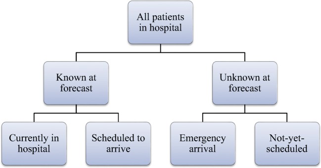
At any future period t, each patient in a hospital will either be known at current period d or unknown. At period d, all known patients existing at period t will either already be in the hospital or scheduled to arrive on or before period t. All remaining patients in the hospital at period t that were not known of at period d are either emergency arrivals, or patients who have not yet been added to the schedule, but will be scheduled to arrive on or before period t. Figure 1 shows these patient groups and their hierarchy.
Fig. 1.
Patient groups in the bed demand forecast
Let represent the forecasted random variable of demand at period t made from period d for a given patient group, where group ∈ {curr, sch, emer, nysched}, representing current patients, scheduled patients, emergency patients, and not-yet-scheduled patients, respectively. Forecasts must be made for each of these patient groups individually and then aggregated to produce the overall patient demand forecast. All patient arrivals and LOS probabilities are assumed to be independent of one another.
Current patients
Each current patient i ∈ M, where M represents the number of current patient types indexed by i, currently in the hospital at period d, either is or is not still in the hospital at future period t, and can thus be represented by a Bernoulli random variable where success is equal to the probability of having a remaining LOS from strictly greater than t − d. Let fi(h) represent the probability of patient i staying exactly h periods from d, meaning the PMF of their remaining LOS is fi(h). Let Fi(h) be the cumulative distribution function (CDF) of fi(h), and Ri(h) = 1 − Fi(h). The probability of patient i still being present at period t when forecasted from period d is represented by Cd, i(t), as shown in Eq. 1.
| 1 |
The convolution of all individual patient probabilities shown in Eq. 1, represented by , is the random variable representing the number of current patients at period d still present at period t. If these patients all have the same probability of being present at period t, then is a Binomial random variable. However, if these probabilities are non-homogeneous, then their convolution follows a Poisson Binomial (PB) distribution [50]. Thus , which represents the random variable representing all current patients at period d being present at period t, follows a PB distribution, with mean and variance as shown in Eqs. 2 and 3, respectively.
| 2 |
| 3 |
Scheduled patients
A patient j ∈ N, where N represents the number of scheduled patient types indexed by j, still being present at the hospital at period t can be represented by a Bernoulli random variable, similar to current patients. Let sj represent the future period on which the patient is scheduled to arrive, such that d + 1 ≤ sj ≤ t. Let fj(h) represent the PMF of staying exactly h periods, Fj(h) be the CDF of fj(h), and Rj(h) = 1 − Fj(h). Then, as represented in Eq. 4, the probability of patient j, scheduled for period sj, being present at period t, when forecasted from period d, is represented by Sd, j(t). Note that h may equal 0.
| 4 |
Similar to current patients, is the convolution of the individual patient distributions shown in Eq. 4, which is the sum of non-homogeneous Bernoulli random variables, and thus PB. The mean and variance of this random variable are represented by Eqs. 5 and 6, respectively.
| 5 |
| 6 |
Emergency patients
Emergency patients arrive at the hospital without ever being scheduled in advance, and are traditionally modeled as Poisson random variables in the literature [51], with a time-varying arrival rate. The arrival rate should be determined for each period, and should thus vary across time. Let the expected number of arrivals on period s, where d + 1 ≤ s ≤ t, of patient type u ∈ U, where U represents the number of emergency patient types indexed by u, be represented by λu(s), and the probability of staying exactly h nights be represented by fu(h), where fu(0) = 0 for all u. Let Fu(h) be the CDF of fu(h), and Ru(h) = 1 − Fu(h). Because both thinning and summing Poisson random variables produces a Poisson random variable, the sum of the expected remaining patients from each previous period’s arrivals is the expected value of a Poisson-distributed variable of the total remaining emergency patients. The number of future emergency patients present at period t, when forecasted from period d, represented by Poisson random variable , has a mean equal to its variance, which is shown in Eq. 7.
| 7 |
Not-yet-scheduled patients
Patients booked at period b to arrive on period s, such that d + 1 ≤ b ≤ s ≤ t, are not-yet-scheduled, but may be present at period t. These patients are unknown, and can thus not be modeled with Bernoulli random variables. There is little research on this topic, though linear regression has been shown to reasonably predict the number of not-yet-scheduled patients [52]. Suppose the number of patients of type v ∈ V, where V represents the number of emergency patient types indexed by v, scheduled on a given booking period b for scheduled period s is Poisson distributed and represented by λv(b, s). The probability of patients of type v staying exactly h nights is represented by fv(h), where fv(0) = 0 for all v. Let Fv(h) be the CDF of fv(h), and Rv(h) = 1 − Fv(h). The random variable representing not-yet-scheduled patients present at period t, with mean and variance as shown in Eq. 8, is thus represented by .
| 8 |
Total demand
Determining the distribution of total demand at period t from forecast period d, represented by Γd(t), requires a convolution of known and unknown patients present at period t. The PMF of current and scheduled patients are PB distributions, meaning the distribution of known patients is also PB, as the sum of two sums of heterogeneous Bernoulli random variables is also a sum of heterogeneous Bernoulli random variables. The PMF of emergency and not-yet-scheduled patients are Poisson, meaning the distribution of unknown patients is also Poisson.
Calculating the full convolution of total patient demand Γd(t), which is the sum of a PB random variable representing known patients, and a Poisson random variable representing unknown patients, is computationally expensive to calculate [53]. This is partly because it has an infinite domain and the number of unique combinations of the PB distribution is equal to 2(M + N), where M + N is the number of known patients, which exceeds one trillion with just 40 known patients. Instead of calculating the complete convolution of Γd(t), an approximation using the normal distribution is obtained using the mean and variance of forecasted patient demand. The mean, as shown in Eq. 9, is the sum of Eqs. 2, 5, 7, and 8, and the variance, as shown in Eq. 10, is the sum of Eqs. 3, 6, 7, and 8. This Normal distribution, as well as the underlying convolution that includes a Poisson distribution, both have infinite domains. These distributions represent the demand for beds, and can thus exceed the hospital unit capacity. When calculating the bed demand, this Normal distribution should be truncated at zero, and when predicting the bed occupancy, this Normal distribution should be truncated at both zero and the hospital unit capacity.
| 9 |
| 10 |
Error calculations
Let the error of the forecast for period t made from period d be represented by ed, t. If At is the actual census for period t, then Eq. 11 shows the calculation for ed, t. The Z-score of the error, represented in Eq. 12 by Zd, t, equals the number of standard deviations away from the forecasted mean and the standard deviation is equal to the square root of the forecast variance.
| 11 |
| 12 |
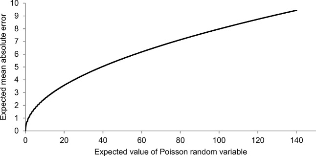
The case where all LOS distributions are deterministic, meaning no uncertainty in LOS, such that all variance comes from unknown future patients, is the theoretical lowest-variance forecast. In this case, the mean and variance of the PB random variable would become an integer constant and zero, respectively. Thus, the distribution of the forecasted PMF with the lowest variance is a translated Poisson random variable that is translated by the amount equal to the expected value of the PB random variable. If a forecast is made equal to the mean of this translated Poisson random variable, then the expected MAE of the forecasted PMF with the lowest variance can be obtained as shown in Eq. 13, where λ + c and λ represent the mean and variance of the translated Poisson (TP) random variable, respectively. The proof is shown in the appendix. Note that ⌊λ⌋ represents the largest integer less than or equal to λ. Translating the Poisson random variable does not affect the expected MAE, and the result in Eq. 13 can be further reduced, as shown in Eq. 14, where fP represents the PMF of a standard Poisson random variable with a mean of λ. To calculate the theoretical best expected value of a multi-period forecast with non-homogenous Poisson random variables, the value in Eq. 14 must be averaged for all periods, using the actual number of arrivals to estimate λ. Figure 2 shows the expected MAE for a single Poisson random variable as a function of λ.
| 13 |
| 14 |
Fig. 2.
Theoretical minimum expected mean absolute deviation of a Poisson random variable
Parameterization
Populating all the necessary parameters for a forecast of T total periods requires significant parameterization and calculation. Table 1 shows the six groups of parameters that must be developed, along with their corresponding indices. These parameters can either be determined from the empirical distribution of the dataset or produced using more powerful methods, such as machine learning. For instance, historical data could populate a logistic regression or decision tree model to estimate the probability of staying any number of nights. Several other works have thoroughly analyzed LOS predictions, and are good resources for this important aspect of forecasting bed demand [13, 49, 37]. Unlike for the other patient groups, fj(0) for scheduled patients must be determined.
Table 1.
Parameters requiring calculation for a forecast of length T from period d
| Parameters | Indices |
|---|---|
| fi(h) | ∀i and h ≥ 1 |
| fj(h) | ∀j and h ≥ 0 |
| fu(h) | ∀u and h ≥ 1 |
| fv(h) | ∀v and h ≥ 1 |
| λu(s) | ∀u and d + 1 ≤ s ≤ d + T |
| λv(b, s) | ∀v and d + 1 ≤ b ≤ s ≤ d + T |
Case study
Blinded de-identified data were obtained for all patients scheduled to arrive or having stayed between 10/31/2015 and 9/16/2016 at a mid-sized Massachusetts community hospital. The next three subsections describe the raw data, develop the model parameters, and produce and analyze the forecast results. This particular application of the model used days as periods to determine the midnight census, and combined all hospital units into a single entity. To assess the performance of the proposed model, a 7-period moving average (MA) model was also developed.
Descriptive analytics
Included in the hospital dataset were about 10,000 patients, 36% of whom were scheduled to arrive, versus 64% of whom were never scheduled. Of the scheduled patients, 26% had a LOS of at least one night, meaning the dataset included about 1000 scheduled inpatient surgeries. The dataset included fields for arrival date, departure date, if the patient was scheduled or not, and for all scheduled patients, fields for booking date, surgeon, and procedure. The mean LOS for scheduled inpatients and emergency patients were 2.5 and 4.1 days, respectfully.
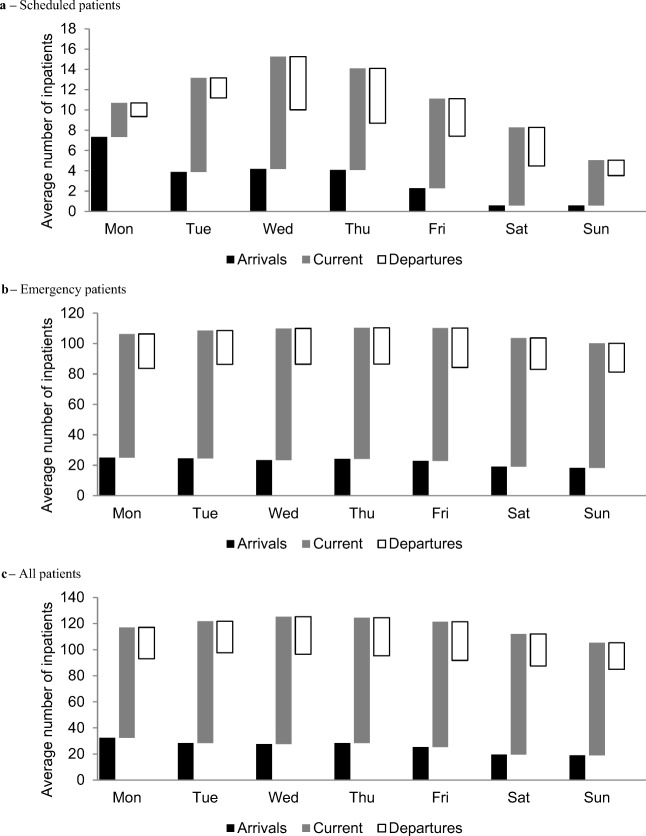
The nightly midnight census is set equal to the sum of new arrivals that day and the current patients that morning, minus the departed patients. Figure 3 shows the mean arrivals, current patients, and departures by DOW in waterfall form, where the bottom of the third bar represents the mean midnight census for that particular DOW. About one-third of all inpatient surgeries occur on Mondays, and taper across the week, with the highest mean of surgical census occurring on Wednesday. Mean emergency patient arrivals also peak on Monday, with the census peaking on Wednesday. Few scheduled inpatient surgeries occur on weekends, whereas the mean number of emergency arrivals is roughly constant by DOW.
Fig. 3.
Average inpatient arrivals and current inpatients and inpatient departures by DOW and split by scheduled and emergency and all patients combined
Model parameterization
Construction of the forecasting model required calculation of the flow probabilities and arrival rates in Table 1. In this case study, seven primary patient types were differentiated: emergency patients and six surgical patients grouped by orthopedic, general surgery, urology, gynecology, neurosurgery, and all other specialties combined.
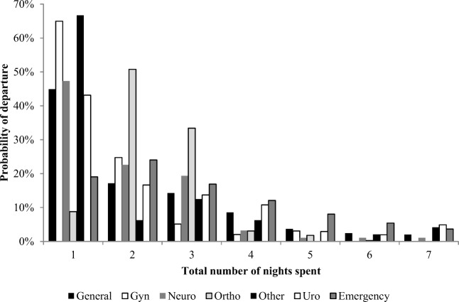
The LOS distribution for emergency patients was set equal to the empirical LOS distribution for all emergency patients. Patients not spending a night in the hospital were excluded from the analysis due to not being part of the midnight inpatient bed census. The LOS distributions for each surgical group were calculated assuming an inpatient stay of at least one night. The probability of a scheduled surgery becoming an inpatient stay was based on the proportion of patients having that particular procedure being an inpatient to the number scheduled. Hence, the LOS distribution was conditioned on staying at least one night, based purely on the procedure, then determined based on the surgical group. Figure 4 shows a bar chart containing the LOS distributions for each patient type, conditioned on staying at least one night, and truncated after seven nights. Due to data availability, the LOS distributions were not updated at each subsequent time period for each patient.
Fig. 4.
LOS distributions conditioned on staying at least one night and truncated after seven nights
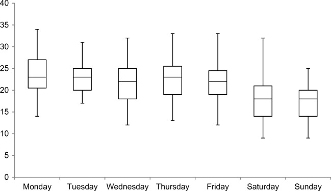
The arrival rates for emergency patients were set equal to the mean number of daily arrivals by DOW. Figure 5 contains box plots showing the arrival distributions by DOW. The bottom and top whiskers represent the minimum and maximum values, respectively, the centerlines represent the medians, and the bottom and top of the boxes represent the 25th and 75th percentiles. Arrival rates for not-yet-scheduled patients were set to the empirical distribution of scheduled patients by surgical group, appointment DOW, and the number of days between the booking date and the appointment date.
Fig. 5.
Arrival distributions for emergency patients
Forecast results
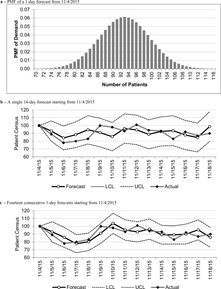
From each date between 10/31/2015 and 8/26/2016, the patient volume was forecasted 14 days into the future, representing 301 forecasts for each of the 14 lengths. Figure 6a shows the forecasted 1-day PMF of demand from 11/4/2015 to 11/5/2015, based on the discrete Normal approximation using the mean and variance of demand. Figure 6b shows an example of a single 14-day forecast starting from 11/4/2015 versus the actual values, and Fig. 6c shows fourteen consecutive 1-day forecasts starting from 11/4/2015 versus the actual values. The lower control limits (LCL) and upper control limits (UCL) are drawn two standard deviations below and above the means in both figures, respectively, where the standard deviation is set to the square root of the forecasted variance.
Fig. 6.
A 1-day forecasted PMF followed by a comparison of a single 14-day forecast to fourteen consecutive 1-day forecasts for the same period
From each day d, forecasts were made with a total length of 14 days, meaning T = 14. For each of the forecasted lengths, the MAE was calculated, as well as the mean and standard deviation of the Z-scores of the errors. These results are shown in Table 2, in addition to the theoretical minimum expected MAE as determined by Eq. 14. The theoretical MAE is calculated by setting λ equal to the actual number of unknown daily arrivals and taking the mean of the daily expected MAE. The simple 7-period MA model had a MAE of 6.0 for a 1-period forecast, representing a 17% increase in error compared to the proposed model.
Table 2.
Experimental results of the 14 forecast lengths with 301 forecasts each
| Forecast Length | MAE of daily expected value | Mean of Z-scores | SD of Z-scores | ||
|---|---|---|---|---|---|
| Observed | Theoretical | Difference | |||
| 1 | 5.1 | 3.7 | 1.4 | −0.01 | 1.02 |
| 2 | 6.5 | 5.0 | 1.5 | −0.02 | 1.02 |
| 3 | 6.9 | 5.7 | 1.2 | −0.02 | 0.98 |
| 4 | 7.1 | 6.2 | 0.9 | −0.03 | 0.96 |
| 5 | 7.3 | 6.5 | 0.8 | −0.04 | 0.99 |
| 6 | 7.5 | 6.7 | 0.8 | −0.05 | 1.00 |
| 7 | 7.6 | 6.8 | 0.7 | −0.05 | 1.02 |
| 8 | 7.7 | 7.0 | 0.7 | −0.06 | 1.03 |
| 9 | 7.7 | 7.0 | 0.7 | −0.06 | 1.04 |
| 10 | 7.8 | 7.1 | 0.7 | −0.08 | 1.05 |
| 11 | 7.8 | 7.1 | 0.7 | −0.08 | 1.05 |
| 12 | 7.8 | 7.2 | 0.6 | −0.08 | 1.06 |
| 13 | 7.8 | 7.2 | 0.6 | −0.09 | 1.06 |
| 14 | 7.8 | 7.3 | 0.6 | −0.09 | 1.06 |
Two-sided Z-tests were applied to each forecast length to compare the means of the forecast error Z-scores to zero. They all passed with α = .05, meaning none of the means of the Z-score errors were statistically different than zero. Also using two-sided Z-tests, the means of the squared values of the Z-scores were compared to one for each forecast length. The difference between these values and one were not found to be statistically significant for any of the forecasted lengths. Given that the standard deviation of a random variable is equal to , with E[X2] not statistically different from one, and E[X] not statistically different from zero, it is reasonable to conclude that the standard deviations of the forecasts were not statistically different from one. This finding supports the assumption of patient bed demand following a normal distribution.
In addition to testing the means and standard deviations of the Z-scores of the error, each of the 14 forecast lengths was tested for normality using the Kolmogorov-Smirnov test, in which the null hypothesis was that the forecast distribution was from a normal distribution with mean and variance equal to the forecasted mean and variance. If the test statistic exceeds the critical value, then the null hypothesis is rejected. Otherwise, if the null hypothesis is embraced, then statistical support exists for a normal distribution being a good fit for the true distribution. For all fourteen forecasts lengths, the null hypothesis was embraced at the 5% significance level, which supports the use of normal approximations for future bed demand.
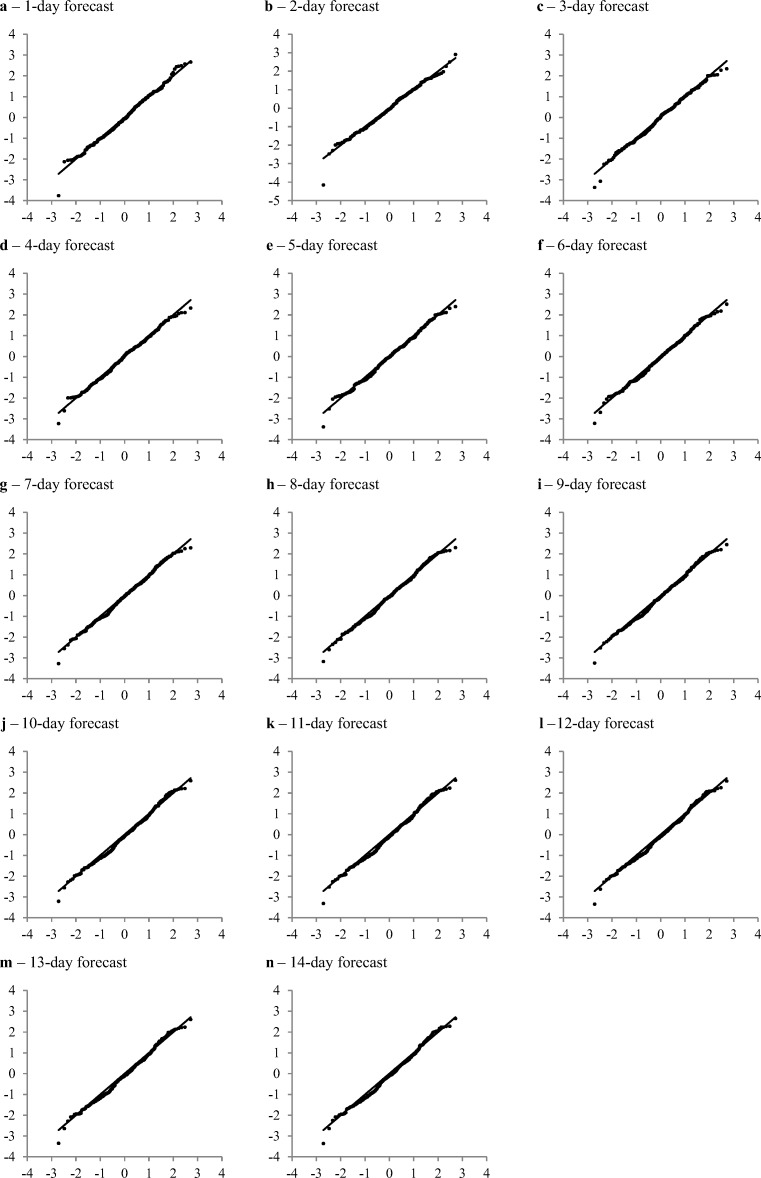
To visually assess the overall fit of the normal approximation, Q-Q plots were created to identify outliers. Q-Q plots are used to compare the empirical distribution percentiles to the theoretical distribution percentiles, as shown in Fig. 7. The x-axis in each plot corresponds to the theoretical normal distribution percentiles, and the y-axis in each plot corresponds to the empirical distribution of the Z-scores of the forecast errors. A 45-degree line is drawn in each chart to show the ideal fit of the two sets of quantiles.
Fig. 7.
Q-Q plots of case study forecasts for 1–14 day lengths where the x-axes represent the theoretical quantiles and the y-axes represent the empirical quantiles
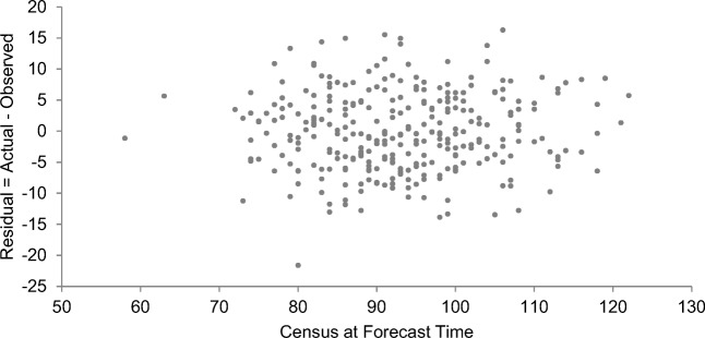
This forecasting model assumes that all arrival rates and LOS distributions are independent, and thus does not take into account system effects like congestion and negative feedback loops. A chi-squared test for independence was prepared to test if the 1-day forecast errors were independent of the census at the time of the forecast. Five bins were created for both the error and the census at the time of the forecast, centered on their respective means, creating a total of 25 bins in the joint distribution. The middle bins represented the mean plus or minus half the standard deviation. The next bin on each side also had a width of a single standard deviation. Values more than 1.5 standard deviations above or below the mean were placed in the highest and lowest bins, respectively. The chi-squared test statistic was equal to 16.4, which with 16 degrees of freedom and α = .05, was not found to be statistically significant, and hence, there was insufficient evidence to demonstrate non-independence. The forecast residuals versus the census at the forecast times are shown in Fig. 8, the distribution of observed values is shown in Table 3, and the distribution of expected values is shown in Table 4.
Fig. 8.
1-day forecast residuals versus census at forecast time
Table 3.
Observed distribution 2-way table showing the joint distribution of 1-day residuals and census at forecast times
| {Min, Max} | Residual = Actual - Observed | ||||||
|---|---|---|---|---|---|---|---|
| < −9.5 | −9.5, −3.2 | −3.2, 3.1 | 3.1, 9.4 | > 9.4 | Total | ||
| Census at Forecast Time | < 76.7 | 1 | 3 | 8 | 3 | 0 | 15 |
| 76.7, 87.6 | 7 | 19 | 27 | 22 | 6 | 81 | |
| 87.6, 98.4 | 5 | 40 | 36 | 24 | 7 | 112 | |
| 98.4, 109.3 | 4 | 15 | 25 | 23 | 4 | 71 | |
| > 109.3 | 1 | 6 | 5 | 10 | 0 | 22 | |
| Total | 18 | 83 | 101 | 82 | 17 | 301 | |
Table 4.
Expected distribution 2-way table showing the joint distribution of 1-day residuals and census at forecast times
| {Min, Max} | Residual = Actual - Observed | ||||||
|---|---|---|---|---|---|---|---|
| < −9.5 | −9.5, −3.2 | −3.2, 3.1 | 3.1, 9.4 | > 9.4 | Total | ||
| Census at Forecast Time | < 76.7 | 0.9 | 4.1 | 5.0 | 4.1 | 0.8 | 15 |
| 76.7, 87.6 | 4.8 | 22.3 | 27.2 | 22.1 | 4.6 | 81 | |
| 87.6, 98.4 | 6.7 | 30.9 | 37.6 | 30.5 | 6.3 | 112 | |
| 98.4, 109.3 | 4.2 | 19.6 | 23.8 | 19.3 | 4.0 | 71 | |
| > 109.3 | 1.3 | 6.1 | 7.4 | 6.0 | 1.2 | 22 | |
| Total | 18 | 83 | 101 | 82 | 17 | 301 | |
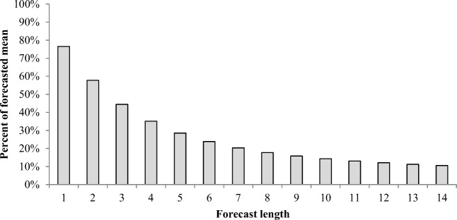
The total population of patients is a combination of known and unknown patients, represented by a PB and Poisson random variable, respectively. Figure 9 shows the average ratio of known patients to all patients from each forecast length, representing the proportion of the forecast that could theoretically be known with close to certainty if LOS distribution predictions improve and approach a smaller variance. As t → ∞, when all known patients will have departed, and only unknown patients remain, the forecast converges to a Poisson random variable. On the first day of the forecast, nearly 80% of the mean of bed demand was from known patients, compared to just 20% on the seventh day.
Fig. 9.
Percent of the mean from known patients for each forecast length
Discussion
This paper demonstrates a novel and accurate method to produce a multi-day forecast of the PMF of hospital bed demand. The case study results are promising, including an MAE close to the theoretical minimum expected MAE, means of error Z-scores close to zero, standard deviations of error Z-scores close to one, and successful Kolmogorov-Smirnov tests for all forecasted lengths. In addition, the chi-squared test for independence demonstrated that forecast residuals were independent of the bed demand at the time of the forecasting, confirming that the assumption of independent patient flow variables was reasonable.
Predictably, the forecasts increase in MAE as their lengths increase, though the difference between the prediction and the theoretical minimum expected MAE decreases. This suggests that although there is room for improvement in predicting the arrival rates for emergency patients and not-yet-scheduled patients, the more significant forecast improvement opportunity lies in predicting (i.e., reducing the variance of the PMF of) the LOS distributions for current and scheduled patients. Improving LOS distributions could be accomplished via real-time updating from electronic medical records, including data on age, gender, medical history, and list of orders, to drive personalized classification and regression models. Furthermore, as natural language processing improves, valuable information from clinician notes may become available for predictive models to improve personalization.
Only 13% of the inpatient stays at this hospital were scheduled, representing only 8% of total nights spent. This relatively low proportion of scheduled patients significantly increases the variance of the theoretical best quality forecast due to the dominance of the Poisson random variable for unknown patients relative to the PB random variable for known patients. Applying the forecasting model to a hospital that predominantly sees scheduled patients relative to emergency patients could significantly reduce the MAE of the predictions. In addition, because the curve in Fig. 2 is concave down, the rate of expected MAE increase is slower than the rate of the increase of the mean of unknown patients, meaning this forecasting model should produce a smaller ratio of MAE to mean census at larger hospitals with similar LOS distributions.
The Q-Q plots in Fig. 7 demonstrate that a normal distribution with the forecasted mean and variance is a suitable estimation of the full probability convolution. The estimations hold well within the range of about two standard deviations, indicated by little deviation from the 45-degree line. However, the 1-day high outliers are above the 45-degree line, indicating that the upper tail of the normal distribution estimate may be too thin to fit the real data. This makes sense given that Poisson distributions have positive skew and most of the forecast is driven by the underlying Poisson random variable for unknown patients. The Q-Q plots for other forecast lengths tend to have high outliers below the 45-degree line, suggesting that consistent multi-day volume increases may be mitigated over several days via reduced LOS or fewer scheduled surgeries. A prominent outlier occurs on the night of June 4th, 2016, when the 1-day forecast from the previous day had an error Z-score of −3.8, and a 2-day forecast Z-score of −4.2. The following day, June 5th, 2016, also clearly shows up on the 3-day Q-Q plot. Although an explanation for this outlier likely exists, tracing its root-cause was beyond the scope of the study.
A potential limitation of this work is the assumption that all random variables are independent of each other, as it is possible that some processes adjust when the census is extreme. For instance, a full hospital may prohibit non-critical short-term scheduling, or demonstrate a greater urgency to discharge current patients to make room for new ones. Although the chi-squared test demonstrated independence between the census at the time of the forecast and the next day’s forecast residual, incorporating system-level adjustments in future forecast model expansion work may enhance the quality of the predictions in extreme cases.
Another limitation is that the parameterization could benefit from the application of machine learning algorithms and additional data, especially data that is updated during the patient visit. For instance, learning that a patient has moved to the ICU or is on a ventilator would significantly increase the expected remaining LOS. Incorporating natural language processing to read the clinician notes would further improve the accuracy of the patient-level parameters. The difference in accuracy between the case study accuracy and theoretical best accuracy demonstrates the value in improving these parameters. As these parameter errors compound, the gap between the theoretical best accuracy and the model accuracy widens. Furthermore, error can exist within the input parameters themselves, in addition to the inherent error of any probability not equaling zero or one. This model assumes that probabilistic input parameters have been accurately determined, and an opportunity for future work would be to analyze the effect of poor parameter estimation on the aggregate demand prediction.
Future work could improve this model by incorporating unit-level flows and a joint distribution of demand across these units by addressing unit-level transfers, as well as including resource demand ratios to produce a PMF of resource demand. For instance, beyond predicting the demand for beds, which is a one-to-one relationship to patients, the model could be expanded to predict the need for nurses and technicians in specific units, who can cover multiple patients based on severity and needs. The ultimate intent is to apply a stochastic optimization model that sets base level staffing and adjusts it based on a pool of shared resources based on a joint probability distribution of demand across all units. In addition to expanding the detail of the model structure and parameters, the full convolution of demand could be integrated to improve the predicted PMF accuracy.
Conclusion
An accurate forecasting model has been derived and implemented that generalizes previous models in the literature by allowing multi-period forecasts, PMFs of demand instead of point estimates, non-cyclic surgery schedules, time-varying LOS distributions, and patient heterogeneity. In a case study, the forecasts held up to statistical tests of independence and normality. This forecasting method allows bed managers significantly more information, both in accuracy and timeliness, to adapt staffing levels to stochastic demand, potentially leading to cost reduction and safety improvements. Most significantly, this work demonstrates a theoretical minimum error in a single-unit bed demand forecast, which can be used to assess the accuracy of future work in this domain.
Appendix
Calculation of expected MAE of a translated Poisson random variable given its mean (λ + c) and variance (λ).
Split the sums along λ + c and k.
Combine the sums without the extra k in the sum.
Add and subtract identical sums to get (k − c) in the sums that used to have just k.
Adjust sums by c.
Combine terms.
Simplify.
Simplify.
Simplify.
To calculate the expected value of the daily expected MAE across multiple days, sum this value across all days and divide by n.
Contributor Information
Samuel Davis, Email: davis.sam@husky.neu.edu.
Nasser Fard, Email: n.fard@neu.edu.
References
- 1.GRUEN R. To Err Is Human. Eds. L. T. Kohn, J. M. Corrigan and M. S. Donaldson. National Academy Press Washington, D.C. 2000. Pp. 287. $34.95. Epidemiol Infect. 2001;126(1):312. [Google Scholar]
- 2.Needleman J, Buerhaus P, Pankratz VS, Leibson CL, Stevens SR, Harris M. Nurse Staffing and Inpatient Hospital Mortality. N Engl J Med. 2011;364(11):1037–1045. doi: 10.1056/NEJMsa1001025. [DOI] [PubMed] [Google Scholar]
- 3.McGillis Hall L, Doran D, Pink GH. Nurse Staffing Models, Nursing Hours, and Patient Safety Outcomes. J Nurs Adm. 2004;34(1):41–45. doi: 10.1097/00005110-200401000-00009. [DOI] [PubMed] [Google Scholar]
- 4.Cochran JK, Broyles JR. Developing nonlinear queuing regressions to increase emergency department patient safety: Approximating reneging with balking. Comput Ind Eng. 2010;59(3):378–386. [Google Scholar]
- 5.Hoot NR, Zhou C, Jones I, Aronsky D. Measuring and Forecasting Emergency Department Crowding in Real Time. Ann Emerg Med. 2007;49(6):747–755. doi: 10.1016/j.annemergmed.2007.01.017. [DOI] [PMC free article] [PubMed] [Google Scholar]
- 6.Zeng Z, Ma X, Hu Y, Li J, Bryant D. A Simulation Study to Improve Quality of Care in the Emergency Department of a Community Hospital. J Emerg Nurs. 2012;38(4):322–328. doi: 10.1016/j.jen.2011.03.005. [DOI] [PubMed] [Google Scholar]
- 7.Peck JS, Benneyan JC, Nightingale DJ, Gaehde SA. Predicting emergency department inpatient admissions to improve same-day patient flow. Acad Emerg Med. 2012;19(9):1045–1054. doi: 10.1111/j.1553-2712.2012.01435.x. [DOI] [PubMed] [Google Scholar]
- 8.Kadri F, Harrou F, Chaabane S, Tahon C. Time series modelling and forecasting of emergency department overcrowding. J Med Syst. 2014;38(9):107. doi: 10.1007/s10916-014-0107-0. [DOI] [PubMed] [Google Scholar]
- 9.Connelly LG, Bair AE. Discrete event simulation of emergency department activity: A platform for system-level operations research. Acad Emerg Med. 2004;11(11):1177–1185. doi: 10.1197/j.aem.2004.08.021. [DOI] [PubMed] [Google Scholar]
- 10.Azari-Rad S, Yontef A, Aleman DM, Urbach DR. A simulation model for perioperative process improvement. Oper Res Heal Care. 2014;3(1):22–30. [Google Scholar]
- 11.Wang B, Han X, Zhang X, Zhang S. Predictive-reactive scheduling for single surgical suite subject to random emergency surgery. J Comb Optim. 2015;30(4):949–966. [Google Scholar]
- 12.Fügener A, Hans EW, Kolisch R, Kortbeek N, Vanberkel PT. Master surgery scheduling with consideration of multiple downstream units. Eur J Oper Res. 2014;239(1):227–236. [Google Scholar]
- 13.Littig SJ, Isken MW. Short term hospital occupancy prediction. Health Care Manag Sci. 2007;10(1):47–66. doi: 10.1007/s10729-006-9000-9. [DOI] [PubMed] [Google Scholar]
- 14.Kumar A, Jiao RJ, Shim SJ (2008) Predicting bed requirement for a hospital using regression models. In: 2008 IEEE International Conference on Industrial Engineering and Engineering Management, IEEM 2008, pp. 665–669
- 15.Abraham G, Byrnes GB, Bain CA. Short-term forecasting of emergency inpatient flow. IEEE Trans Inf Technol Biomed. 2009;13(3):380–388. doi: 10.1109/TITB.2009.2014565. [DOI] [PubMed] [Google Scholar]
- 16.Kortbeek N, Braaksma A, Smeenk FHF, Bakker PJM, Boucherie RJ. Integral resource capacity planning for inpatient care services based on bed census predictions by hour. J Oper Res Soc. 2015;66(7):1061–1076. [Google Scholar]
- 17.McManus ML, Long MC, Cooper A, Litvak E. Queuing Theory Accurately Models the Need for Critical Care Resources. Anesthesiology. 2004;100(5):1271–1276. doi: 10.1097/00000542-200405000-00032. [DOI] [PubMed] [Google Scholar]
- 18.Verburg IWM, De Keizer NF, De Jonge E, Peek N. Comparison of regression methods for modeling intensive care length of stay. PLoS One. 2014;9(10):e109684. doi: 10.1371/journal.pone.0109684. [DOI] [PMC free article] [PubMed] [Google Scholar]
- 19.Cahill W, Render M. Dynamic simulation modeling of ICU bed availability. WSC’99 1999 Winter Simul Conf Proceedings ‘Simulation - A Bridg to Futur (Cat No99CH37038) 1999;2:1573–1576. [Google Scholar]
- 20.Troy PM, Rosenberg L. Using simulation to determine the need for ICU beds for surgery patients. Surgery. 2009;146(4):608–620. doi: 10.1016/j.surg.2009.05.021. [DOI] [PubMed] [Google Scholar]
- 21.McConnell KJ, Richards CF, Daya M, Bernell SL, Weathers CC, Lowe RA. Effect of increased ICU capacity on emergency department length of stay and ambulance diversion. Ann Emerg Med. 2005;45(5):471–478. doi: 10.1016/j.annemergmed.2004.10.032. [DOI] [PubMed] [Google Scholar]
- 22.Zhu Z, Hoon Hen B, Liang Teow K. Estimating ICU bed capacity using discrete event simulation. Int J Health Care Qual Assur. 2012;25(2):134–144. doi: 10.1108/09526861211198290. [DOI] [PubMed] [Google Scholar]
- 23.Gholipour C, Rahim F, Fakhree A, Ziapour B. Using an artificial neural networks (ANNS) model for prediction of intensive care unit (ICU) outcome and length of stay at hospital in traumatic patients. J Clin Diagn Res. 2015;9(4):19–23. doi: 10.7860/JCDR/2015/9467.5828. [DOI] [PMC free article] [PubMed] [Google Scholar]
- 24.Tierney LT, Conroy KM. Optimal occupancy in the ICU: A literature review. Aust Crit Care. 2014;27(2):77–84. doi: 10.1016/j.aucc.2013.11.003. [DOI] [PubMed] [Google Scholar]
- 25.Marmor YN, Rohleder TR, Cook DJ, Huschka TR, Thompson JE. Recovery bed planning in cardiovascular surgery: a simulation case study. Health Care Manag Sci. 2013;16(4):314–327. doi: 10.1007/s10729-013-9231-5. [DOI] [PubMed] [Google Scholar]
- 26.Rohleder TR, Lewkonia P, Bischak DP, Duffy P, Hendijani R. Using simulation modeling to improve patient flow at an outpatient orthopedic clinic. Health Care Manag Sci. 2011;14(2):135–145. doi: 10.1007/s10729-010-9145-4. [DOI] [PubMed] [Google Scholar]
- 27.Pan C, Zhang D, Kon AWM, Wai CSL, Ang WB. Patient flow improvement for an ophthalmic specialist outpatient clinic with aid of discrete event simulation and design of experiment. Health Care Manag Sci. 2015;18(2):137–155. doi: 10.1007/s10729-014-9291-1. [DOI] [PubMed] [Google Scholar]
- 28.Liu N, Ziya S, Kulkarni VG. Dynamic Scheduling of Outpatient Appointments Under Patient No-Shows and Cancellations. Manuf Serv Oper Manag. 2010;12(2):347–364. [Google Scholar]
- 29.Xie H, Chaussalet TJ, Millard PH. A continuous time Markov model for the length of stay of elderly people in institutional long-term care. J R Stat Soc Ser A Stat Soc. 2005;168(1):51–61. [Google Scholar]
- 30.Zhang Y, Puterman ML, Nelson M, Atkins D (2012) A Simulation Optimization Approach to Long-Term Care Capacity Planning A Simulation Optimization Approach to Long-Term Care Capacity Planning
- 31.Joy MP, Jones S (2005) Predicting bed demand in a hospital using neural networks and ARIMA models: a hybrid approach. In: 13th European Symposium on Artificial Neural Networks, pp. 27–29
- 32.Xu Q, Tsui KL, Jiang W, Guo H. A Hybrid Approach for Forecasting Patient Visits in Emergency Department. Qual Reliab Eng Int. 2016;32(8):2751–2759. [Google Scholar]
- 33.Weiss EN, Cohen MA, Hershey JC. An Iterative Estimation and Validation Procedure for Specification of Semi-Markov Models with Application to Hospital Patient Flow. Oper Res. 1982;30(6):1082–1104. doi: 10.1287/opre.30.6.1082. [DOI] [PubMed] [Google Scholar]
- 34.Andersen AR, Nielsen BF, Reinhardt LB. Optimization of hospital ward resources with patient relocation using Markov chain modeling. Eur J Oper Res. 2017;260(3):1152–1163. [Google Scholar]
- 35.Pagel C, et al. Development, implementation and evaluation of a tool for forecasting short term demand for beds in an intensive care unit. Oper Res Heal Care. 2017;15:19–31. [Google Scholar]
- 36.Green LV, Nguyen V. Strategies for cutting hospital beds: The impact on patient service. Health Serv Res. 2001;36(2):421–442. [PMC free article] [PubMed] [Google Scholar]
- 37.Armony M, Israelit S, Mandelbaum A, Marmor YN, Tseytlin Y, Yom-Tov GB. On Patient Flow in Hospitals: A Data-Based Queueing-Science Perspective. Stoch Syst. 2015;5(1):146–194. [Google Scholar]
- 38.Harrison GW, Shafer A, Mackay M. Modelling Variability in Hospital Bed Occupancy. Health Care Manag Sci. 2005;8(4):325–334. doi: 10.1007/s10729-005-4142-8. [DOI] [PubMed] [Google Scholar]
- 39.Steins K, Walther SM. A generic simulation model for planning critical care resource requirements. Anaesthesia. 2013;68(11):1148–1155. doi: 10.1111/anae.12408. [DOI] [PubMed] [Google Scholar]
- 40.Konrad R, et al. Modeling the impact of changing patient flow processes in an emergency department: Insights from a computer simulation study. Oper Res Heal Care. 2013;2(4):66–74. [Google Scholar]
- 41.Choon OH, Dali Z, Beng PT, Magdalene CPY. Uncovering effective process improvement strategies in an emergency department using discrete event simulation. Heal Syst. 2014;3(2):93–104. [Google Scholar]
- 42.Dexter F, Macario A, Traub RD, Hopwood M, Lubarsky DA. An operating room scheduling strategy to maximize the use of operating room block time: Computer simulation of patient scheduling and survey of patients’ preferences for surgical waiting time. Anesth Analg. 1999;89(1):7–20. doi: 10.1097/00000539-199907000-00003. [DOI] [PubMed] [Google Scholar]
- 43.Blasak RE, Armel WS, Starks DW, Hayduk MC. The use of simulation to evaluate hospital operations between the emergency department and a medical telemetry unit. Proc 2003 Winter Simul Conf 2003. 2003;2:1887–1893. [Google Scholar]
- 44.Günal MM, Pidd M. Discrete event simulation for performance modelling in health care: A review of the literature. J Simul. 2010;4(1):42–51. [Google Scholar]
- 45.Day TE, et al. Addressing the variation of post-surgical inpatient census with computer simulation. Pediatr Surg Int. 2014;30(4):449–456. doi: 10.1007/s00383-014-3475-0. [DOI] [PubMed] [Google Scholar]
- 46.Hoot NR, et al. Forecasting Emergency Department Crowding : A Discrete Event Simulation. Ann Emerg Med. 2008;52(2):116–125. doi: 10.1016/j.annemergmed.2007.12.011. [DOI] [PMC free article] [PubMed] [Google Scholar]
- 47.Resar R, Nolan K, Kaczynski D, Jensen K. Using real-time demand capacity management to improve hospitalwide patient flow. Jt Comm J Qual Patient Saf. 2011;37(5):217–227. doi: 10.1016/s1553-7250(11)37029-8. [DOI] [PubMed] [Google Scholar]
- 48.Marshall A, Vasilakis C, El-Darzi E. Length of stay-based patient flow models: Recent developments and future directions. Health Care Manag Sci. 2005;8(3):213–220. doi: 10.1007/s10729-005-2012-z. [DOI] [PubMed] [Google Scholar]
- 49.Harrison GW, Escobar GJ. Length of stay and imminent discharge probability distributions from multistage models: variation by diagnosis, severity of illness, and hospital. Health Care Manag Sci. 2010;13(3):268–279. doi: 10.1007/s10729-010-9128-5. [DOI] [PubMed] [Google Scholar]
- 50.Hoeffding Wassily. On the Distribution of the Number of Successes in Independent Trials. The Annals of Mathematical Statistics. 1956;27(3):713–721. [Google Scholar]
- 51.Young JP. Stabilisation of inpatient bed occupancy through control of admissions. Hospitals (Lond) 1965;39(19):41–48. [PubMed] [Google Scholar]
- 52.Graue RM (2013) Prediction and optimization techniques to streamline surgical scheduling
- 53.Hong Y. On computing the distribution function for the Poisson binomial distribution. Comput Stat Data Anal. 2013;59:41–51. [Google Scholar]


