

Abstract
The Tofts pharmacokinetic model requires multiple calculations for analysis of dynamic contrast enhanced (DCE) MRI. In addition, the Tofts model may not be appropriate for the prostate. This can result in error propagation that reduces the accuracy of pharmacokinetic measurements. In this study, we present a compact solution allowing estimation of physiological parameters Ktrans and ve from ultrafast DCE acquisitions, without fitting DCE-MRI data to the standard Tofts pharmacokinetic model. Since the standard Tofts model can be simplified to the Patlak model at early times when contrast efflux from the extravascular extracellular space back to plasma is negligible, Ktrans can be solved explicitly for a specific time. Further, ve can be estimated directly from the late steady-state signal using the derivative form of Tofts model. Ultrafast DCE-MRI data were acquired from 18 prostate cancer patients on a Philips Achieva 3T-TX scanner. Regions-of-interest (ROIs) for prostate cancer, normal tissue, gluteal muscle, and iliac artery were manually traced. The contrast media concentration as function of time was calculated over each ROI using gradient echo signal equation with pre-contrast tissue T1 values, and using the ‘reference tissue’ model with a linear approximation. There was strong correlation (r = 0.88–0.91, p < 0.0001) between Ktrans extracted from the Tofts model and Ktrans estimated from the compact solution for prostate cancer and normal tissue. Additionally, there was moderate correlation (r = 0.65–0.73, p < 0.0001) between extracted versus estimated ve. Bland-Altman analysis showed moderate to good agreement between physiological parameters extracted from the Tofts model and those estimated from the compact solution with absolute bias less than 0.20 min−1 and 0.10 for Ktrans and ve, respectively. The compact solution may decrease systematic errors and error propagation, and could increase the efficiency of clinical workflow. The compact solution requires high temporal resolution DCE-MRI due to the need to adequately sample the early phase of contrast media uptake.
Keywords: pharmacokinetic models, physiological parameters, arterial input function, ultrafast dynamic contrast enhanced MRI
1. Introduction
Dynamic contrast enhanced (DCE) MRI plays an important role in the detection, diagnosis and staging of cancers (Abramson et al 2013, Chandarana et al 2013, Vos et al 2013, Pinker et al 2014, Tan et al 2015, Tong et al 2015, Dijkhoff et al 2017). DCE-MRI is usually acquired with a series of T1-weighted (T1w) spoiled gradient echo images before, during and after IV bolus injection of gadolinium (Gd)-based contrast media (Buckley et al 2004, Larsson et al 2008). The DCE-MRI data can be analyzed visually or semi-quantitatively, or quantitatively using pharmacokinetic models (Brix et al 1991, Tofts 1997, Kuhl et al 1999, Jansen et al 2010, Petrillo et al 2015). The most common pharmacokinetic models used in the literature are the standard or extended Tofts models (Tofts 1997, Tofts et al 1999), which extract the volume transfer constant (Ktrans) between blood plasma and the extravascular extracellular space (EES) and the fractional volume of EES (ve). Use of pharmacokinetic models requires calculation of contrast media concentration in tissue as a function of time (C(t)) based on T1w imaging signal intensity (S(t)).
There are multiple ways to calculate C(t) in tissue, including: (i) using the gradient echo signal equation (nonlinear model) with pre-contrast tissue T1 values (often measured with variable flip angle technique) (Dale et al 2003); and (ii) using the ‘reference tissue’ model under linear approximation (Medved et al 2004). Both of these techniques have advantages and disadvantages. Theoretically speaking, C(t) calculated from the non-linear model is more accurate than the linear ‘reference tissue’ model, but its precision is strongly influenced by the native T1 values (Cernicanu and Axel 2006, Di Giovanni et al 2010). The variable flip angle technique which is frequently used to measure pre-contrast tissue T1 values contributes error to calculations of C(t) using the nonlinear model (Preibisch and Deichmann 2009, Hurley et al 2012). These errors are likely to propagate through the computationally complex calculations required to extract Ktrans and ve using the Tofts model. This affects the accuracy of extracted parameters (Garpebring et al 2013). In addition, extra scans for B1 correction and measurement of the native T1 extend the time required for the MRI protocol (Pineda et al 2016).
Previous studies have demonstrated the advantages of high temporal resolution DCE-MRI for improving lesion conspicuity (Rosenkrantz et al 2015). High temporal resolution DCE-MRI also improves quantitative analysis because arterial input function (AIF) and tissue contrast media uptake can be sampled more accurately (Parker et al 2006, Garpebring et al 2009, Jena et al 2017). There are several studies proposing new methods to improve calculation of physiological parameter maps (Murase 2004, Garpebring et al 2009, Yuan et al 2012, Vajuvalli et al 2014). For examples, Murase (2004) developed a technique that integrates differential equations and converts them to a matrix form, then solves them using the linear least-squares method. Garpebring et al (2009) and Vajuvalli et al (2014) proposed techniques that utilize calculations in the Fourier domain and/or frequency analysis. Although the Fourier transform is a fast and powerful approach in study of pharmacokinetic models, the accuracy of Fourier based methods is limited by the smoothness of the change in contrast media concentration as a function of time (Vajuvalli et al 2016). In addition, all these methods require calculation of tissue contrast media concentration. Simplified and robust methods using signal intensity may provide more accurate estimates of physiologic parameters.
In this study, a new compact solution based on the standard Tofts model (Tofts et al 1999) was developed for estimating physiological parameters. The purpose of the study was to compare physiological parameters estimated from proposed compact solution to those extracted from the standard Tofts model, in human prostate DCE-MRI data. The compact solution is particularly appropriate in this setting since very high temporal resolution for DCE-MRI (~2 seconds per image) facilitates use of the unidirectional (Patlak) approximation (Patlak and Blasberg 1985), when data from only the early phase of contrast media uptake is used. This avoids unnecessary assumptions regarding the number and nature of tissue compartments in the microenvironment and thus further reduces error.
2. Materials and methods
2.1. Theory
Based on the standard Tofts model of DCE-MRI, the change in contrast media concentration (C(t)) as a function of time (t) in tissue following bolus contrast media injection is given by Tofts et al (1999):
| (1) |
where Ktrans is the volume transfer constant between blood plasma and extravascular extracellular space (EES), ve is the volume of EES per unit volume of tissue, Cp(t) = Cb(t)/(1 − Hct) is the arterial input function (AIF), Cb(t) is contrast media concentration in blood, Hct is the hematocrit (=0.42), and τ0 is the delay between the arrival of contrast media in AIF and in tissue. At earlier times after contrast media injection (t ≪ 1min), the efflux of the contrast media from the EES back to plasma is negligible, and equation (1) can be simplified as Patlak and Blasberg (1985):
| (2) |
Equation (2) works well when data are acquired at very high temporal resolution, since at early times, flow is approximately unidirectional. Then for a specific time, the Ktrans can either be solved for directly or by taking the derivatives with respect to time on both sides of equation (2), as demonstrated by Bennink et al (2013):
| (3a) |
| (3b) |
By using the linear ‘reference tissue’ model (Medved et al 2004), C(t) can be approximated from the signal intensity S(t) as a function of time when a reference tissue with a known native T1 (T1ref), such as muscle or adipose tissue, is available, i.e.
| (4) |
where r1 is the longitudinal relaxivity of the contrast media, and S(0) and Sref(0) are the tissue and reference tissue signal intensities before contrast media injection, respectively. This approximation works particularly well during the early phase of contrast media uptake when the tissue contrast media concentration is relatively low, T1 is relatively long, and magnetization is highly saturated (Medved et al 2004). Combining equation (3) and (4), the following formula can be obtained:
| (5a) |
| (5b) |
Where , and Sb(t) is the signal intensity in blood. For a specific time soon after contrast media injection, t = tp, the integral or derivative in equation (5) can be evaluated numerically for estimation of Ktrans. Here, the specific time ‘tp’ must be early enough for the Patlak approximation to hold. At the same time, the signal-to-noise ratio (SNR) of signal enhancement at ‘tp’ must be adequate.
To estimate ve, the following derivative form of the standard Tofts model is employed (Tofts et al 1999):
| (6) |
At longer times after contrast media injection (t ≫ 1min), it is a good approximation that dC(t)/dt ≈ 0 because C(t) changes very slowly (He et al 2017). Then equation (6) can be simplified as:
| (7) |
For a specific later time, t = tN, ve can be estimated as follows by replacing C(t) in equation (7) with S(t) in equation (4):
| (8) |
Please note that if the measurements at t = tN are made before the blood and tissue contrast media concentrations reach a steady state, then equation (8) may overestimate or underestimate ve compared to the value for ve obtained from fitting with the Tofts model. In this study, the early time post injection tp was selected as the time-to-peak of the AIF, and tN was the time of the final post-contrast image.
2.2. Human prostate DCE-MRI acquisition
In this retrospective study, human prostate DCE-MRI data were used to compare the physiological parameters estimated by the new techniques described above and those extracted directly from the Tofts model. Patients provided prior informed written consent under a protocol approved by our Institutional Review Board and compliant with Health Insurance Portability and Accountability Act. Patients were excluded if they had previously received radiation or hormonal replacement therapy (leading to alterations in prostatic signal on MRI), if their glomerular filtration rate measured less than 60 ml min−1/1.73 m2, or if there were any other contraindications to MRI. As a result, eighteen patients with prior biopsy proven prostate cancer were included in this study and were imaged prior to surgery between January and December 2016. The mean age of patients was 60 years (range 47–70 years) and mean PSA was 8.4 ng ml−1 (range 3.7–31.9 ng ml−1).
The MRI data were acquired on a Philips Achieva 3T-TX scanner (Philips Healthcare, Netherlands) with d-Stream RF technology using a six-channel phased array surface coil (Medrad, Bayer Healthcare), coupled with an integrated posterior coil. Immediately before imaging, 1 mg of glucagon was injected intramuscularly. After other clinically necessary scans, such as axial T2-weighted (T2w) imaging and diffusion-weighted imaging were completed, a T1 mapping sequence was acquired before administration of contrast media using variable flip angle 3D T1-weighted (T1w) fast field echo (FFE) (TR/TE = 12/2.3 ms, field of view = 385 × 250 mm, matrix size = 308 × 220, flip angle = 3°, 5°, 10°, 15°, 20°, 30°, slice thickness = 3.5 mm, typical number of slices = 24, SENSE factor = 1.67, half scan factor = 0.675). Subsequently, DCE 3D T1-FFE data was acquired (TR/TE = 3.5/1.0 ms, field of view = 180 × 180 mm, matrix size = 160 × 160, flip angle = 10°, slice thickness = 3 mm, typical number of slices = 24, SENSE factor = 3.5, half scan factor = 0.625) for 150 dynamic scan points. The temporal resolution ranged from 1.0–4.3 s depending on the number of imaging slices needed to cover the whole prostate, with 2.2 s being the typical value. A dose of 0.1 mmol kg−1 of contrast media gadoterate meglumine (DOTAREM®, Guerbet LLC, Bloomington, IN, USA) was injected beginning at the ~10th dynamic scan point with an injection rate of 2.0 ml s−1 followed by a 20 ml saline flush.
2.3. Data analysis
Human prostate DCE-MRI data was analyzed using MATLAB (MathWorks, Natick, MA) with an in-house software package. MRI and H&E stained whole mount radical prostatectomy sections were matched by consensus of an experienced radiologist (AO) and pathologist (TA) to guide selection of cancer and normal regions of interest (ROIs). ROIs in prostate cancers and normal tissue over different prostate zones were drawn on T2w trans-axial images and transferred to DCE images based on H&E stained whole mount prostatectomy specimens. The ROIs for blood vessels were manually traced on DCE images over the cross section of the iliac artery on the MRI slice containing cancer. In addition, a gluteal muscle ROI was traced on DCE images for each patient. For each ROI, the average DCE-MRI signal intensity as a function of time (S(t)) was calculated. The native T1 in each ROI was calculated by using the pre-contrast variable flip angle images as previously described (Manuel et al 2011, Pineda et al 2016). The contrast media concentration as a function of time (C(t)) was calculated using a previously published method based on the gradient echo signal equation (non-linear model) (Dale et al 2003). The AIF (Cp(t)) was determined from the signal intensity in the iliac artery.
For each tissue ROI, the physiological parameters were extracted first from the standard Tofts model by fitting equation (1), and then (5) and (8) were used to estimate the physiological parameters Ktrans and ve. The transit delay between the time-of-initial enhancement in the artery and tissue was accounted for by shifting the arterial signal such that the initial arterial enhancement matched that of the tissue in order to use equations (5) and (8). The shift time τ0 in the AIF was optimized so that the standard Tofts model fits best matched C(t). Since the derivative in equation (5) can be very sensitive to noise and is hard to calculate accurately, an empirical mathematical model (EMM) previously found to accurately fit a wide range of contrast media uptake and washout curves (Fan et al 2004) was used to fit S(t) and subsequently the derivative was obtained from the EMM-fitted S(t).
Pearson’s correlation coefficient was calculated between physiological parameters (Ktrans and ve) extracted from the standard Tofts model and estimated from the compact solution. Bland-Altman analysis was performed to evaluate the agreement between extracted and estimated Ktrans and ve values. A p -value less than 0.05 was considered statistically significant.
3. Results
A total of forty-four cancer ROIs (16 Gleason score 3 + 3, 22 Gleason score 3 + 4, 5 Gleason score 4 + 3, 1 Gleason score 4 + 5), 18 gluteal muscle ROIs, and sixty-three normal prostate tissue ROIs from different zones: 16 peripheral zone (PZ), 15 transition zone (TZ), 16 central zone (CZ), and 16 anterior fibromuscular stroma (AFMS) were used in this study. The average (±standard deviation (SD)) τ0 was 5.15 ± 2.26, 5.35 ± 3.02, 4.38 ± 2.82 s for gluteal muscle, normal prostate tissues, and prostate cancers, respectively.
Figure 1 illustrates the steps used to compare physiological parameters extracted from the Tofts model versus those estimated from the presented compact solution for a typical case. Figure 1(A) shows measured signal intensities S(t) for blood vessel and cancer ROIs. The corresponding calculated contrast media concentration C(t) is shown in figure 1(B). Figure 1(C) shows the integration (gray area) of Sb(t) between t0 (time of zero) and tp (time to peak of AIF), the derivative at S(tp) (slope) used for estimation of Ktrans, and S(tN) was used for estimation of ve. Figure 1(D) shows the Ktrans and ve values extracted from the Tofts model compared with values estimated from our compact solution.
Figure 1.

Steps used to compare conventionally extracted physiological parameters from the Tofts model versus estimated physiological parameters from our compact solution, as illustrated in a 65 year old subject with cancer (Gleason 4 + 5). (A) The signal intensities Sb(t) (red circles) and S(t) (black squires) measured for arterial blood (red arrow) and cancer (yellow arrow), respectively. (B) Calculated Cp(t) for AIF (red line) and C(t) for cancer (black line) from the signal intensity curves, as well as Tofts model fits to cancer C(t) (green line). (C) The integration (gray area) of Sb(t) between t0 (time of 0) and tp (time to peak of AIF), the derivative at S(tp) (slope) used for estimation of Ktrans, and S(tN) used for estimation of ve. (D) The results of extracted and estimated physiological parameters for this subject.
Figures 2 and 3(A1)–(A3) show scatter plots of extracted Ktrans from the Tofts model versus estimated Ktrans from our compact solution using the integral (figure 2) and derivative (figure 3) formulas for different ROIs: (A1) gluteal muscle, (A2) normal prostate tissue, and (A3) prostate cancers. There was moderate to strong positive correlations (r = 0.56–0.91, p < 0.0001) between extracted versus estimated Ktrans. The corresponding Bland-Altman plots for these Ktrans are shown in figures 2 and 3(B1)–(B3). For most cases, there were good agreements between extracted and estimated Ktrans with bias of −0.03 to −0.20 min−1, except for a few ROIs that are close to or beyond the limits of agreements.
Figure 2.

Scatter plots (top row) of Ktrans extracted from Tofts model versus Ktrans obtained from the integral formula in equation (5a) for (A1) muscle, (A2) prostate tissue, and (A3) prostate cancers. The lines represent the linear correlations. The corresponding Bland-Altman plots are shown in the bottom row (B1)-(B3). The solid line represents the mean difference (extracted-estimated) and the dashed gray lines represent the lower and upper limits of agreement, defined by a range of ±1.96 × SD (95% confidence interval) around the mean difference.
Figure 3.
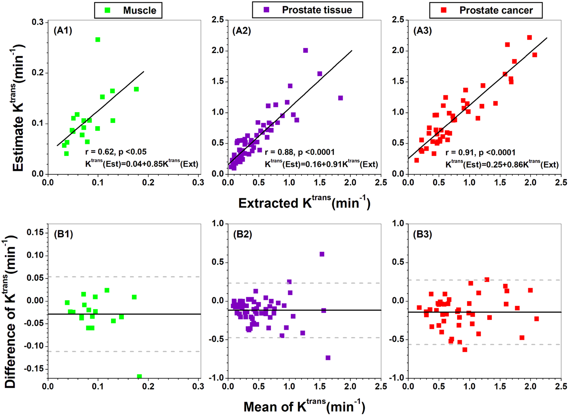
Scatter plots (top row) of Ktrans extracted from Tofts model versus Ktrans obtained from the derivative formula in equation (5b) for (A1) muscle, (A2) prostate tissue, and (A3) prostate cancers. The lines represent the linear correlations. The corresponding Bland-Altman plots are shown in the bottom row (B1)-(B3). The solid line represents the mean difference (extracted-estimated) and the dashed gray lines represent the lower and upper limits of agreement, defined by a range of ±1.96 × SD (95% confidence interval) around the mean difference.
Finally, figure 4 shows scatter plots of ve from the Tofts model versus estimated ve from our compact solution using equation (8) for different ROIs: (A1) gluteal muscle, (A2) normal prostate tissue, (A3) prostate cancers. There was weak to moderate positive correlations (r = 0.45–0.73, p = 0.07 to < 0.001) between extracted versus estimated ve. The corresponding Bland-Altman plots for ve are shown in figures 4(B1)–(B3). In five cases for normal prostate tissue and seven cases for prostate cancer, the estimated ve was larger than 1.0, which is physiologically unrealistic.
Figure 4.

Scatter plots (top row) of ve extracted from Tofts model versus ve obtained from the compact solution (equation (8)) for (A1) muscle, (A2) prostate tissue, and (A3) prostate cancers. The lines represent the linear correlations. The corresponding Bland-Altman plots are shown in the bottom row (B1)-(B3). The solid line represents the mean difference (extracted-estimated) and the dash gray lines represent the lower and upper limits of agreement, defined by a range of ±1.96 × SD (95% confidence interval) around the mean difference.
4. Discussion
Ultrafast DCE-MRI data from human prostate were used to validate our compact solution for estimation of physiological parameters in cancer and normal prostate tissue ROIs selected on the MRI scans based on histology of prostatectomy specimens. Overall agreement between values obtained from the compact solution and from the Tofts model was good, especially for Ktrans. The main advantage of the compact solution is that the physiological parameters could be estimated by using signal intensity as function of time curve and without fitting the Tofts model to reduce error propagation, as well as systematic error.
When the Tofts model is used to fit C(t), the need to fit the entire curve may result in suboptimal estimates of values of Ktrans and ve particularly in normal prostate and prostate cancer, where a simple two-compartment model may not be appropriate (Franiel et al 2008, Schimpf et al 2017). In contrast, our compact solution estimates physiological parameters using only S(t) at very early times and very late times after contrast media injection. This avoids assumptions about the compartmental structure of the tissue that may lead to systematic errors in physiologic parameters.
The compact solution is most accurate during the early phase of contrast media uptake when contrast media concentration is low, the tissue T1 is relatively long, and therefore magnetization is highly saturated (Medved et al 2004). Thus the compact model is compatible with ultrafast sampling, and use of the unidirectional flow model, which requires data acquired at early times after contrast media injection.
The ve can be estimated using very sparse DCE-MRI sampling in the washout phase. However, the model (equation (8)) used to estimate ve could overestimate or underestimate ve compared with directly fitting with the Tofts model, if measurements are made before the blood and tissue contrast media concentrations reach a steady state. The underlining assumption used in equation (8) is that the derivative of S(t) is close to zero at t = tN. This was the reason that there were 12 cases with estimated ve larger than 1.0. Our prostate DCE-MRI data was not acquired long enough to follow contrast media washout until a steady-state between blood and tissue was reached.
There were several limitations to this study. First, our sample size is small and the compact solution requires testing in a much larger and more diverse group of patients. In addition, the compact solution can be applied only to estimate parameters accurately if data are acquired with ultrafast DCE-MRI. The temporal resolution of DCE-MRI should be less than 5 s so that the AIF and initial contrast media uptake can be adequately sampled (Parker et al 2006). Second, the compact solution is strongly influenced by the time point selected for the calculations, since we are assuming approximately unidirectional flow. The time to peak of AIF used in our estimations may not have been optimal. An earlier point in the early uptake phase may have been more consistent with the unidirectional flow approximation. The trade-off between selecting earlier time points and maintaining adequate SNR will be investigated in later work. Third, errors in measurement of the delay time (τ0) between the arrival of contrast media in arteries and tissue can result in significant errors in estimated physiological parameters (Chouhan et al 2016). We are working to develop a more accurate algorithm for estimation of τ0. Fourth, noise in the data contributes errors to the integral and derivative used in the compact solution. In this study, we used the EMM to fit the S(t) so that the derivative could be more accurately calculated. This avoids the use of a two compartment model, and the need for convolution. Finally, in the current study, Ktrans and ve were estimated from single data points. Errors in estimated Ktrans could be further reduced by using several data points before the peak of the AIF to calculate an average Ktrans. To minimize errors in ve, contrast media washout could be sampled over a longer period, and the mean signal from several data points at the later times could be used in calculations.
5. Conclusion
In summary, the compact solution presented here could simplify calculation of physiological parameters Ktrans and ve in ultrafast DCE-MRI acquisitions and may reduce error propagation. Since no compartmental model is required, the compact solution is likely to work well for tissues with complex compartmental structure, such as normal and cancerous prostate. It avoids errors in fitting data using the standard Tofts pharmacokinetic model.
Acknowledgments
This research is supported by the National Institutes of Health (Grant Nos: R01CA218700, U01CA142565, R01CA172801 and S10OD018448), the University of Chicago Comprehensive Cancer Center from the National Cancer Institute Cancer Center Support Grant P30CA014599 and the Fundamental Research Funds for the Central Universities (No. 02120022119001).
References
- Abramson RG, Li X, Hoyt TL, Su PF, Arlinghaus LR, Wilson KJ, Abramson VG, Chakravarthy AB and Yankeelov TE 2013. Early assessment of breast cancer response to neoadjuvant chemotherapy by semi-quantitative analysis of high-temporal resolution DCE-MRI: preliminary results Magn. Reson. Imaging 31 1457–64 [DOI] [PMC free article] [PubMed] [Google Scholar]
- Bennink E, Riordan AJ, Horsch AD, Dankbaar JW, Velthuis BK and De Jong HW 2013. A fast nonlinear regression method for estimating permeability in CT perfusion imaging J. Cereb. Blood Flow Metab 33 1743–51 [DOI] [PMC free article] [PubMed] [Google Scholar]
- Brix G, Semmler W, Port R, Schad LR, Layer G and Lorenz WJ 1991. Pharmacokinetic parameters in CNS Gd-DTPA enhanced MR imaging J. Comput. Assist. Tomogr 15 621–8 [DOI] [PubMed] [Google Scholar]
- Buckley DL, Roberts C, Parker GJ, Logue JP and Hutchinson CE 2004. Prostate cancer: evaluation of vascular characteristics with dynamic contrast-enhanced T1-weighted MR imaging-initial experience Radiology 233 709–15 [DOI] [PubMed] [Google Scholar]
- Cernicanu A and Axel L 2006. Theory-based signal calibration with single-point T1 measurements for first-pass quantitative perfusion MRI studies Acad. Radiol 13 686–93 [DOI] [PubMed] [Google Scholar]
- Chandarana H, Amarosa A, Huang WC, Kang SK, Taneja S, Melamed J and Kim S 2013. High temporal resolution 3D gadolinium-enhanced dynamic MR imaging of renal tumors with pharmacokinetic modeling: preliminary observations J. Magn. Reson. Imaging 38 802–8 [DOI] [PubMed] [Google Scholar]
- Chouhan MD, Bainbridge A, Atkinson D, Punwani S, Mookerjee RP, Lythgoe MF and Taylor SA 2016. Estimation of contrast agent bolus arrival delays for improved reproducibility of liver DCE MRI Phys. Med. Biol 61 6905–18 [DOI] [PMC free article] [PubMed] [Google Scholar]
- Dale BM, Jesberger JA, Lewin JS, Hillenbrand CM and Duerk JL 2003. Determining and optimizing the precision of quantitative measurements of perfusion from dynamic contrast enhanced MRI J. Magn. Reson. Imaging 18 575–84 [DOI] [PubMed] [Google Scholar]
- Di Giovanni P, Azlan CA, Ahearn TS, Semple SI, Gilbert FJ and Redpath TW 2010. The accuracy of pharmacokinetic parameter measurement in DCE-MRI of the breast at 3 T Phys. Med. Biol 55 121–32 [DOI] [PubMed] [Google Scholar]
- Dijkhoff RAP, Beets-Tan RGH, Lambregts DMJ, Beets GL and Maas M 2017. Value of DCE-MRI for staging and response evaluation in rectal cancer: a systematic review Eur. J. Radiol 95 155–68 [DOI] [PubMed] [Google Scholar]
- Fan X, Medved M, River JN, Zamora M, Corot C, Robert P, Bourrinet P, Lipton M, Culp RM and Karczmar GS 2004. New model for analysis of dynamic contrast-enhanced MRI data distinguishes metastatic from nonmetastatic transplanted rodent prostate tumors Magn. Reson. Med 51 487–94 [DOI] [PubMed] [Google Scholar]
- Franiel T, Ludemann L, Rudolph B, Rehbein H, Staack A, Taupitz M, Prochnow D and Beyersdorff D 2008. Evaluation of normal prostate tissue, chronic prostatitis, and prostate cancer by quantitative perfusion analysis using a dynamic contrast-enhanced inversion-prepared dual-contrast gradient echo sequence Invest. Radiol 43 481–7 [DOI] [PubMed] [Google Scholar]
- Garpebring A, Brynolfsson P, Yu J, Wirestam R, Johansson A, Asklund T and Karlsson M 2013. Uncertainty estimation in dynamic contrast-enhanced MRI Magn. Reson. Med 69 992–1002 [DOI] [PubMed] [Google Scholar]
- Garpebring A, Ostlund N and Karlsson M 2009. A novel estimation method for physiological parameters in dynamic contrast-enhanced MRI: application of a distributed parameter model using Fourier-domain calculations IEEE Trans. Med. Imaging 28 1375–83 [DOI] [PubMed] [Google Scholar]
- He D, Zamora M, Oto A, Karczmar GS and Fan X 2017. Comparison of region-of-interest-averaged and pixel-averaged analysis of DCE-MRI data based on simulations and pre-clinical experiments Phys. Med. Biol 62 N445–59 [DOI] [PMC free article] [PubMed] [Google Scholar]
- Hurley SA, Yarnykh VL, Johnson KM, Field AS, Alexander AL and Samsonov AA 2012. Simultaneous variable flip angle-actual flip angle imaging method for improved accuracy and precision of three-dimensional T1 and B1 measurements Magn. Reson. Med 68 54–64 [DOI] [PMC free article] [PubMed] [Google Scholar]
- Jansen SA et al. 2010. Characterizing early contrast uptake of ductal carcinoma in situ with high temporal resolution dynamic contrast-enhanced MRI of the breast: a pilot study Phys. Med. Biol 55 N473–85 [DOI] [PubMed] [Google Scholar]
- Jena A, Taneja S, Singh A, Negi P, Mehta SB and Sarin R 2017. Role of pharmacokinetic parameters derived with high temporal resolution DCE MRI using simultaneous PET/MRI system in breast cancer: a feasibility study Eur. J. Radiol 86 261–6 [DOI] [PubMed] [Google Scholar]
- Kuhl CK, Mielcareck P, Klaschik S, Leutner C, Wardelmann E, Gieseke J and Schild HH 1999. Dynamic breast MR imaging: are signal intensity time course data useful for differential diagnosis of enhancing lesions? Radiology 211 101–10 [DOI] [PubMed] [Google Scholar]
- Larsson HB, Hansen AE, Berg HK, Rostrup E and Haraldseth O 2008. Dynamic contrast-enhanced quantitative perfusion measurement of the brain using T1-weighted MRI at 3T J. Magn. Reson. Imaging 27 754–62 [DOI] [PubMed] [Google Scholar]
- Manuel A, Li W, Jellus V, Hughes T and Prasad PV 2011. Variable flip angle-based fast three-dimensional T1 mapping for delayed gadolinium-enhanced MRI of cartilage of the knee: need for B1 correction Magn. Reson. Med 65 1377–83 [DOI] [PubMed] [Google Scholar]
- Medved M, Karczmar G, Yang C, Dignam J, Gajewski TF, Kindler H, Vokes E, Maceneany P, Mitchell MT and Stadler WM 2004. Semiquantitative analysis of dynamic contrast enhanced MRI in cancer patients: variability and changes in tumor tissue over time J. Magn. Reson. Imaging 20 122–8 [DOI] [PubMed] [Google Scholar]
- Murase K 2004. Efficient method for calculating kinetic parameters using T1-weighted dynamic contrast-enhanced magnetic resonance imaging Magn. Reson. Med 51 858–62 [DOI] [PubMed] [Google Scholar]
- Parker GJ, Roberts C, Macdonald A, Buonaccorsi GA, Cheung S, Buckley DL, Jackson A, Watson Y, Davies K and Jayson GC 2006. Experimentally-derived functional form for a population-averaged high-temporal-resolution arterial input function for dynamic contrast-enhanced MRI Magn. Reson. Med 56 993–1000 [DOI] [PubMed] [Google Scholar]
- Patlak CS and Blasberg RG 1985. Graphical evaluation of blood-to-brain transfer constants from multiple-time uptake data. Generalizations J. Cereb. Blood Flow Metab 5 584–90 [DOI] [PubMed] [Google Scholar]
- Petrillo A, Fusco R, Petrillo M, Granata V, Sansone M, Avallone A, Delrio P, Pecori B, Tatangelo F and Ciliberto G 2015. Standardized Index of Shape (SIS): a quantitative DCE-MRI parameter to discriminate responders by non-responders after neoadjuvant therapy in LARC Eur. Radiol 25 1935–45 [DOI] [PubMed] [Google Scholar]
- Pineda FD, Medved M, Fan X and Karczmar GS 2016. B1 and T1 mapping of the breast with a reference tissue method Magn. Reson. Med 75 1565–73 [DOI] [PMC free article] [PubMed] [Google Scholar]
- Pinker K et al. 2014. Clinical application of bilateral high temporal and spatial resolution dynamic contrast-enhanced magnetic resonance imaging of the breast at 7 T Eur. Radiol 24 913–20 [DOI] [PubMed] [Google Scholar]
- Preibisch C and Deichmann R 2009. Influence of RF spoiling on the stability and accuracy of T1 mapping based on spoiled FLASH with varying flip angles Magn. Reson. Med 61 125–35 [DOI] [PubMed] [Google Scholar]
- Rosenkrantz AB et al. 2015. Dynamic contrast-enhanced MRI of the prostate with high spatiotemporal resolution using compressed sensing, parallel imaging, and continuous golden-angle radial sampling: preliminary experience J. Magn. Reson. Imaging 41 1365–73 [DOI] [PMC free article] [PubMed] [Google Scholar]
- Schimpf O, Hindel S and Ludemann L 2017. Assessment of micronecrotic tumor tissue using dynamic contrast-enhanced magnetic resonance imaging Phys. Med 34 38–47 [DOI] [PMC free article] [PubMed] [Google Scholar]
- Tan CH, Hobbs BP, Wei W and Kundra V 2015. Dynamic contrast-enhanced MRI for the detection of prostate cancer: meta-analysis AJR Am. J. Roentgenol 204 W439–48 [DOI] [PMC free article] [PubMed] [Google Scholar]
- Tofts PS 1997. Modeling tracer kinetics in dynamic Gd-DTPA MR imaging J. Magn. Reson. Imaging 7 91–101 [DOI] [PubMed] [Google Scholar]
- Tofts PS et al. 1999. Estimating kinetic parameters from dynamic contrast-enhanced T(1)-weighted MRI of a diffusable tracer: standardized quantities and symbols J. Magn. Reson. Imaging 10 223–32 [DOI] [PubMed] [Google Scholar]
- Tong T, Sun Y, Gollub MJ, Peng W, Cai S, Zhang Z and Gu Y 2015. Dynamic contrast-enhanced MRI: use in predicting pathological complete response to neoadjuvant chemoradiation in locally advanced rectal cancer J. Magn. Reson. Imaging 42 673–80 [DOI] [PubMed] [Google Scholar]
- Vajuvalli NN, Chikkemenahally DK, Nayak KN, Bhosale MG and Geethanath S 2016. The Tofts model in frequency domain: fast and robust determination of pharmacokinetic maps for dynamic contrast enhancement MRI Phys. Med. Biol 61 8462–75 [DOI] [PubMed] [Google Scholar]
- Vajuvalli NN, Nayak KN and Geethanath S 2014. Accelerated pharmacokinetic map determination for dynamic contrast enhanced MRI using frequency-domain based Tofts model Conf. Proc. IEEE Engineering in Medicine and Biology Society pp 2404–7 [DOI] [PubMed] [Google Scholar]
- Vos EK, Litjens GJ, Kobus T, Hambrock T, Hulsbergen-Van De Kaa CA, Barentsz JO, Huisman HJ and Scheenen TW 2013. Assessment of prostate cancer aggressiveness using dynamic contrast-enhanced magnetic resonance imaging at 3 T Eur. Urol 64 448–55 [DOI] [PubMed] [Google Scholar]
- Yuan J, Chow SK, King AD and Yeung DK 2012. Heuristic linear mapping of physiological parameters in dynamic contrast-enhanced MRI without T(1) measurement and contrast agent concentration J. Magn. Reson. Imaging 35 916–25 [DOI] [PubMed] [Google Scholar]