Climate-driven aerobic habitat loss in the California Current System

Aerobic habitat mediates species responses to historical and future climate change in the California Current System.

Abstract

Climate warming is expected to intensify hypoxia in the California Current System (CCS), threatening its diverse and productive marine ecosystem. We analyzed past regional variability and future changes in the Metabolic Index (Φ), a species-specific measure of the environment’s capacity to meet temperature-dependent organismal oxygen demand. Across the traits of diverse animals, Φ exhibits strong seasonal to interdecadal variations throughout the CCS, implying that resident species already experience large fluctuations in available aerobic habitat. For a key CCS species, northern anchovy, the long-term biogeographic distribution and decadal fluctuations in abundance are both highly coherent with aerobic habitat volume. Ocean warming and oxygen loss by 2100 are projected to decrease Φ below critical levels in 30 to 50% of anchovies’ present range, including complete loss of aerobic habitat—and thus likely extirpation—from the southern CCS. Aerobic habitat loss will vary widely across the traits of CCS taxa, disrupting ecological interactions throughout the region.

INTRODUCTION

Hypoxia in the California Current System

Climate change is warming the oceans, depleting its dissolved oxygen (O₂), lowering its pH, and altering species distributions, phenology, and interactions (1). Understanding how these changes affect species fitness remains a challenge for at least two fundamental reasons. First, the role of climate in shaping habitat is mediated by numerous physiological and ecological traits that are not systematically measured and are difficult to disentangle. Second, the observational records needed to detect climate-driven ecosystem changes rarely span the decadal periods of intrinsic ocean variability (2). Attributing past species responses to multiple climate stressors is essential to projecting future climate impacts on marine ecosystems.

The California Current System (CCS) is ideally situated to detect and attribute ecological responses to climate change. Upwelling of nutrient-rich water maintains high biological productivity and ecological diversity, but also bathes the continental shelf in waters that are naturally low in O₂ and pH, two primary stressors for many species (3). The CCS is also a region of strong interannual and decadal hydrographic variability driven by modes of natural climate variability spanning the Pacific Ocean (4). Ecological responses to this climate variability have been observed in species that form critical links in the food web (5–7). These low-frequency perturbations provide “natural experiments” that presage future climate change, and can therefore be used to calibrate thresholds for species and ecosystem responses to accelerating ocean changes.

The CCS is also uniquely suited to evaluate the role of temperature-dependent hypoxia as a driver of global marine habitat loss (8–10). Oxygen loss is projected to be especially strong in the Northeast Pacific, emerging early from the background natural variability there (2). Recent analyses of physiological traits of diverse marine species demonstrate a close alignment of biogeographic range boundaries with the ratios of organismal O₂ supply and demand. This suggests that species geographic ranges are commonly limited by temperature-dependent aerobic energy availability (8). However, this ecophysiological framework, the “Metabolic Index,” has not been tested against ecological observations of species abundance changes over decadal scales. Meanwhile, O₂ fluctuations in the CCS have been statistically implicated in the historical variability of fish populations (5–7), but have yet to be linked to habitat availability based on measurable physiological traits. Here, we use the Metabolic Index to provide evidence of such a link, and present a general approach to evaluate the response of species in a region likely to undergo rapid intensification of temperature-dependent hypoxia in coming decades.

The Metabolic Index and aerobic habitat

The influences of temperature and O₂ on organism fitness are closely linked through the physiology of aerobic respiration. As temperatures rise, most species become less tolerant of low-O₂ water (10), because metabolic O₂ demand rises with temperature faster than organismal O₂ supply does. The temperature-dependent ratio of the potential O₂ supply to metabolic demand can be represented by the Metabolic Index [Φ; (8, 9)], which must exceed a critical value (Φ_crit) for an environment to be ecologically habitable

$$\mathrm{\Phi }=\frac{\text{Supply}}{\text{Demand}}=A_{\mathrm{o}}\frac{p{\mathrm{O}}_2}{\text{exp}(-E_{\mathrm{o}}/k_{\mathrm{B}}(1/T-1/T_{\text{ref}}))}\ge {\mathrm{\Phi }}_{\text{crit}}$$ (1)

This index incorporates both environmental temperature (T, K) and the partial pressure of O₂ (pO₂, atm), as well as species-specific physiological traits. The coefficient A_o (atm⁻¹) is the ratio of oxygen supply to demand by an organism at a reference temperature (T_ref), and measures hypoxia tolerance. The change in hypoxia tolerance with temperature is described by the Arrhenius function (k_B is the Boltzmann constant), with the parameter E_o (eV) representing the temperature sensitivity of hypoxia tolerance. These two physiological parameters—hypoxia tolerance (A_o) and its temperature sensitivity (E_o)—can be calibrated using laboratory experiments, in which the lowest pO₂ that sustains resting metabolism (Φ = 1) is measured over a range of temperatures.

The hypoxia tolerance of an organism in a natural environment is reduced by the additional O₂ needed to sustain critical ecological activity such as movement, feeding, growth, and reproduction. The factor by which hypoxia tolerance is reduced by ecological activity is equal to the ratio of sustained active metabolic rates to those at rest. As a result, for habitat to be aerobically suitable, Φ must also meet or exceed this ratio, termed Φ_crit. We refer to the ratio A_o/Φ_crit as the ecological hypoxia tolerance (versus the resting hypoxia tolerance, A_o). The threshold Φ_crit depends on each species’ ecology and life history in its natural environment, and is inferred from the biogeographic distribution of a species as it spans gradients in Φ. The frequency distribution of biogeographically-inferred Φ_crit (9) is indistinguishable from that of experimentally determined ratios of sustained to resting metabolic rates [Sustained Metabolic Scope; (11)], and ranges from 1.5 to 7 among marine and terrestrial animals (9, 11).

For any species defined by a given set of E_o, A_o, and Φ_crit, hereafter referred to as an ecophysiotype, the volume of water in which Φ ≥ Φ_crit defines the availability of aerobically suitable habitat. Below this critical threshold, Φ represents an energetic constraint on the depth and geographic bounds beyond which a population cannot be sustained. Changes in Φ could influence population abundance through at least three distinct mechanisms. First, a reduction in Φ may eliminate previously occupied aerobic habitat, confining the species to a fraction of its historical range. Absent an increase in population density within the remaining habitable volume, the total abundance over that historical range must also decline. Second, compression of aerobically suitable habitat may alter mortality, for example by confining populations to shallower depths with increased risk of visual predation (5, 12), or may alter the availability of food by shifting populations to less productive regions (13). Finally, because Φ represents the potential aerobic energy supply, a reduction in Φ may diminish activity, thus slowing individual growth and reproduction, even if Φ remains above Φ_crit, and mortality and food availability are constant.

Empirical relationships between Φ and long-term changes in species abundance, should they be detected, would thus suggest a role for temperature-dependent hypoxia in population dynamics, even though the precise mediating factors cannot be identified. To date, shifts in species abundance and range boundaries have been empirically linked to climate variability [e.g., (5, 14)] but have not been attributable to the physiological and ecological traits that regulate aerobic habitat.

Study approach

Our study objectives are threefold: First, we evaluate the role of historical climate variability in modulating aerobic habitat availability in time and space across the CCS. Second, we test whether aerobic habitat constraints can simultaneously account for the long-term biogeographic distribution and decadal variability in abundance of a key CCS species, northern anchovy (Engraulis mordax), with rich historical observations. Third, we use dynamically downscaled climate simulations for the CCS to project the loss of aerobic habitat for northern anchovy, and across the full range of global species’ Metabolic Index parameter space.

To evaluate the relationships between climate variability and species response requires datasets with extent, duration, and resolution greater than what is typically measured, even in the relatively well-sampled CCS. Thus, our approach is to pair complementary observational datasets with ocean model simulations, to increase data resolution with minimal loss of empirical fidelity. Details are summarized diagrammatically in fig. S1 and described in the Materials and Methods following the Discussion.

For hydrographic data, we combine long-term (multidecadal) measurements at coarse spatial and temporal resolution with high-resolution model simulations covering shorter (monthly to interannual) periods of ocean variability. Distributions of hydrographic variables such as temperature and O₂ over the CCS were reconstructed from Regional Ocean Modeling System (ROMS) simulations that were validated with historical hydrographic observations [fig. S2 and Supplementary Materials; (15–18)].

For biological data, we similarly use both the large-scale time-averaged spatial distribution of adult and larval anchovy and highly resolved, long-term time series observations of larval anchovy over a smaller region of the CCS.

We also use the physiological (E_o, A_o) and ecological (Φ_crit) traits from a global compilation of >60 marine species (9) to map the spatial and temporal variability of the Metabolic Index and resulting aerobic habitat across the CCS. These taxonomically diverse species are found in the full range of ocean temperature and O₂ conditions, and yield well-defined frequency distributions of Φ traits. The traits for 14 species found in the CCS (native or introduced; table S1) span much of the global range of traits. We therefore expect the global distribution of ecophysiotypes to characterize unsampled CCS species as well.

Inferring drivers of species responses to climate and other environmental changes has a rich history—and a mixed record of success—in ecology generally and fisheries oceanography in particular. Our approach attempts to avoid the primary pitfalls of such analyses [e.g., (19, 20)] in several ways. First, we base our analysis on spatially resolved environmental conditions at the locations where populations are living, rather than on large-scale climate indices [e.g., regional winds and the Pacific Decadal Ooscillation; (4)] whose local environmental manifestations may be weak or unknown. Second, we choose the environmental conditions (temperature and O₂) because their biological influence is well established and rooted in physiological mechanisms [e.g., (10)]. As a result, while our results necessarily rely partly on correlations, they are correlations with an a priori biological basis. Third, the reliability of our conclusions is based on multiple independent lines of evidence, namely the consistency between the traits that predict historical spatial distribution and the temporal variability of anchovy and their Metabolic Index.

Despite the advantages of this approach, we recognize that even relationships that account for past changes in species abundance can still lead to poor predictions of the future. Our results are thus best interpreted as an imperfect projection based on the current understanding of temperature-dependent hypoxia, the available hydrographic and biological data, and the fidelity of climate models. A discussion of whether alternative mechanisms can explain the historical patterns, and of the caveats involved in projecting the future are elaborated following the results.

RESULTS

Aerobic habitat in the CCS

For typical species traits, the Metabolic Index spans a wide range across the CCS, and has varied strongly over the past several decades (Fig. 1). The spatial patterns of Φ for a commonly observed ecophysiotype (Fig. 1, A to C) are illustrative of those faced by most species, although the absolute values and strength of the gradients vary across traits. In the surface mixed layer, pO₂ is approximately constant and so changes in Φ are driven primarily by temperature, leading to a poleward increase in Φ. At greater depths (e.g., 200 m; Fig. 1A), the increase of Φ with latitude diminishes, as the temperature gradient weakens while the pO₂ gradient remains generally small alongshore. However, near-zero O₂ associated with the Eastern Tropical North Pacific oxygen deficient zone results in a marked, low-Φ boundary at the southern margin of the CCS, and would restrict the equatorward extent of most ecophysiotypes.

Fig. 1. Metabolic Index (Φ) distribution and historical variability in the CCS.

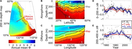
Φ is computed using physiological parameters (hypoxia tolerance A_o = 25 atm⁻¹, temperature sensitivity E_o = 0.4 eV) that are typical of marine species, including those found in the CCS, and for environmental conditions (temperature and O₂) from ROMS model simulations. (A) Mean Φ at 200 m depth, and (B) alongshore depth section (200 km from shore; 12 km resolution hindcast). (C) Offshore depth section (from 4 km resolution ROMS hindcast). Distributions of Φ remain qualitatively similar for species with alternate physiological parameters: Values of Φ scale uniformly higher for species with a higher hypoxia tolerance (higher A_o), whereas for species whose hypoxia tolerance is more temperature sensitive (i.e., higher E_o), vertical Φ gradients are weaker and latitudinal Φ gradients are stronger. In the Southern California Bight, CalCOFI monthly Φ anomalies (for A_o = 30 atm⁻¹, E_o = 0.6 eV) are calculated from historical hydrographic observations at (D) 0 to 200 m depth and (E) 200 to 400 m depth. Data are overlaid by 3-year moving averages of Φ (lines) where both temperature and O₂ vary as observed, as well as Φ expected from changes in temperature or O₂ independently.

Both pO₂ and temperature decrease with depth over the upper ~1000 m, causing both organismal O₂ supply and demand to decrease. However, for nearly all known ecophysiotypes, the intensity of O₂ undersaturation in the mesopelagic (the O₂ minimum zone) causes O₂ supply to decline with depth faster than demand, leading to decreasing Φ with depth throughout the CCS (Fig. 1B). Upwelling and shoaling of deeper offshore water onto the shelf lead to a nearshore reduction of Φ (Fig. 1C). Thus, O₂ explains the major features in the distribution of Φ below the surface (and its variability; fig. S3). On the basis of these spatial patterns, in the coastal CCS aerobic limitation will generally constrain how close to shore and how deep a species can access habitat, in addition to the latitudinal limits. While some strongly temperature-sensitive traits reduce aerobic suitability in the epipelagic subtropical gyre, Φ is not limiting offshore for most ecophysiotypes.

Changes in Φ over time are influenced by both O₂ and temperature variability in comparable measure in the upper 200 m (Fig. 1D), becoming dominated by O₂ changes at deeper depths (Fig. 1E). The time scales of hydrographic variability that drive fluctuations in Φ also vary across depth, with shallower waters exhibiting strong interannual to decadal fluctuations, and deeper mesopelagic waters having a more multidecadal period. Thus, a given climate forcing within the CCS may yield a wide range of species-specific changes in aerobic habitat depending on a species’ depth range and ecophysiotype.

We used the modeled distribution of Φ to assess volumes of available habitat (Fig. 2A) and their variability in time (Fig. 2B) for the upper water column of the coastal CCS for diverse ecophysiotypes. Across the traits for all known species, lower hypoxia tolerance (A_o) reduces aerobically viable habitat volume. This can be compensated in part by species whose hypoxia tolerance is more temperature-dependent (larger E_o), which allows colder waters at depth or higher latitudes to remain habitable even with a lower A_o. The CCS is partially habitable for most species across the global range of traits, implying that this range should encompass traits for CCS species adapted to local environmental conditions. Native CCS species with known Φ_crit (filled symbols in Fig. 2A; primarily deepwater species) have lower active to resting energy demands than the global mean value, increasing available aerobic habitat for a given A_o and E_o.

Fig. 2. Aerobic habitat in the CCS for varied marine ecophysiotypes.

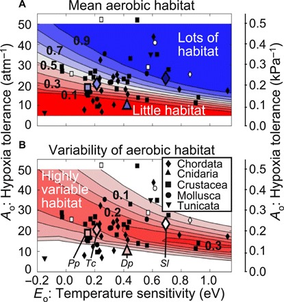
(A) Time-mean aerobic habitat volume and (B) variability in time of aerobic habitat volume (standard deviation), spatially averaged as a fraction of the total volume over the coastal, epipelagic CCS (27°N to 51°N, 0 to 200 km offshore, 0 to 200 m depth; 4 km resolution ROMS hindcast). The range of hypoxia tolerance, A_o, and temperature sensitivity, E_o, evaluated are based on a global species trait compilation; known species traits are marked with black symbols for specific (sub)phyla (legend). This calculation assumes a ratio of active to resting metabolic rates Φ_crit = 3.5, near the inter-specific mean. Native CCS species are marked with open symbols, or, if the species-specific Φ_crit is known, with a larger marker and fill color corresponding to the actual aerobic habitat volume in the specified depth range (Dp, Desmophyllum pertusum; Pp, Pandalus platyceros; Sl, Stenobrachius leucopsarus; Tc, Tarletonbeania crenularis). Lower Φ_crit results in higher aerobic habitat volume for the same physiological traits.

The long-term availability of habitat volume is closely connected to its changes over time (Fig. 2B). Habitat is most variable for ecophysiotypes for which Φ is similar to Φ_crit (with intermediate habitat availability), because small changes in O₂ and temperature can lead to large shifts in habitat availability. Within 200 km of the coast, 30 to 50% of aerobic habitat variability is seasonal, and the rest interannual to interdecadal. Across ecophysiotypes, both habitat availability and variability increase slightly with latitude in the CCS (fig. S3). Habitat integrated over the upper 100 or 400 m exhibits a similar trait dependence as for the upper 200 m. Thus, any species inhabiting the upper 400 m of the CCS with traits typical of global species experiences significant variability in aerobic habitat availability on both seasonal and climatic time scales.

Aerobic habitat constraints on species distributions and variability

To test whether variations in aerobic habitat could have driven species responses to historical climate variability in the CCS, we examined northern anchovy, a key CCS species for which both adult spatial distributions (21, 22) and time variability in larval abundance (23) have been relatively well sampled. Previous studies have used the California Cooperative Oceanic Fisheries Investigations (CalCOFI) time series to show that the abundance of epipelagic and mesopelagic fish larvae in the Southern California Bight (SCB) is correlated with thermocline O₂ (5, 6, 24). We hypothesize that changes in aerobic habitat are the primary underlying driver for changes in the distribution of anchovy. While hypoxia traits for northern anchovy have not been published, this hypothesis gains considerable traction if both the time-mean spatial distribution and the temporal variability of this species can be explained with a single set of Metabolic Index parameters within the range of known species. Such an ecophysiotype offers a testable, quantitative prediction for the likely range of traits for this species.

Climatological patterns

Northern anchovy are found from Baja California to Vancouver Island (Fig. 3A). The greatest concentrations of adult anchovy have historically been observed within 30 km of shore and from 0 to 100 m depth (25), although individuals and schools have been identified at greater depth, particularly over regions of steep bathymetry.

Fig. 3. Anchovy distributions and abundance predicted by the Metabolic Index (Φ).

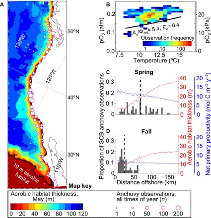
(A) Anchovy observations (circles, n = 1917 from 1888 to 2015, 1° bins), including observations not used in the distribution analysis (all south of 32°N). Also, May aerobic habitat thickness (shading), where Φ ≥ Φ_crit, for the distribution-derived ecophysiotype (from ROMS 12 km resolution climatology, black line contours 10 m thickness). (B) Frequency of anchovy observations associated with climatological O₂ and temperature conditions, for samples paired with observed and modeled hydrographic data (n = 1075, north of 32.63°N only). The resulting temperature-dependent hypoxia threshold for the best-fit ecophysiotype (ecological hypoxia tolerance A_o/Φ_crit = 5.4 atm⁻¹ or 0.053 kPa⁻¹, temperature sensitivity E_o = 0.4 eV or 6 × 10⁻²⁰ J; black line) demarcates the space below which anchovy can sustain resting but not active energetic demands. Cross-shore distributions of anchovy observations, aerobic habitat thickness, and net primary productivity (ROMS 12 km output) in the SCB, in (C) spring, peak upwelling season, and (D) fall. Nearshore aerobic habitat thickness is roughly half as thick, and the mean location of observations (dashed black lines) shifts offshore during upwelling.

We evaluated whether temperature-dependent hypoxia could constrain the historical distribution of this species, using the subset of publicly available anchovy observations which could be closely paired with climatological temperature and O₂ (which included observations from the SCB north; see Materials and Methods). Indeed, the O₂ partial pressures and temperatures bounding anchovy observations are parsimoniously explained by a temperature-dependent critical pO₂ (i.e., Φ/Φ_crit = 1; Fig. 3B). The minimum pO₂, above which anchovy are prevalent and below which occurrences are rare, increases with water temperature. As anchovy inhabit warmer water, they do so only if those waters are also higher in O₂. In contrast, there are no single high-temperature or low-O₂ thresholds that bound the distribution of occupied habitat.

This apparent limit of water properties that anchovy inhabit can be used to diagnose the temperature sensitivity (E_o) and ecological hypoxia tolerance (A_o/Φ_crit, the combined effect of the physiological and ecological constraints). The ability of the Metabolic Index to delineate occupied temperature-O₂ conditions and subsequently predict the observed spatial range of anchovy is a crucial test for the relevance of low Φ to anchovy habitat limits. We distinguish between likely trait combinations using the F1-score, which evaluates how closely an ecophysiotype-predicted limit bounds the actual observations (fig. S4; see Materials and Methods and the Supplementary Materials).

The inferred ecophysiotype with the highest F1-score from the long-term anchovy distribution was A_o/Φ_crit = 5.4 atm⁻¹ (0.053 kPa⁻¹) and E_o = 0.4 eV (6 × 10⁻²⁰ J). Both values are near the mean of known traits for species found in the CCS (table S1). Using this ecophysiotype, we mapped the thickness of aerobic habitat over the entire CCS using a ROMS hindcast of oceanographic conditions from 1995 to 2010 (Fig. 3A). The resulting aerobic habitat encompasses the entire latitudinal range of anchovy observations on at least a seasonal basis—including closely matching the extent of historical anchovy range along Baja California, even though no observations from the southern third of the range were used in the distribution analysis. In other words, the predicted latitudinal range limit based on a subset of the observations closely matches the observed range limit of all observations. Further, the predicted constraints of Φ on the equatorial extent of CCS taxa broadly (Fig. 1A) are consistent with the known distribution of this key species.

The seasonal shifts in the vertical and offshore distribution of anchovy and Φ further support the idea that aerobic habitat constrains anchovy. In both the SCB (Fig. 3, C and D) and northern CCS (fig. S6), anchovy migrate offshore during peak upwelling seasons, which vary with latitude (21, 25, 26). This redistribution occurs when nearshore aerobic habitat availability is lowest (e.g., <10 m aerobic habitat thickness within ~25 km of shore), even though concurrent net primary productivity (a proxy for food supply) is generally highest near shore and lowest offshore.

Descriptions of finer scale seasonal anchovy dispersal in the SCB (25) are also qualitatively consistent with avoidance of seasonally evolving upwelling (27) and associated low O₂, and do not track seasonal or spatial patterns of primary productivity, which is generally greatest in the northern nearshore SCB [e.g., (28)]. Adult anchovy have also been observed to shift tens of meters deeper in winter (25), as Φ_crit similarly deepens. In addition to these within-region movements, tagged fish have been observed to migrate hundreds of kilometers alongshore (29); northward movement is primarily in summer, and southward movement is mostly in the winter when aerobic habitat deepens. Thus, seasonal distributions of anchovy are also qualitatively and quantitatively consistent with aerobic habitat limitation.

Response to decadal climate variability

CalCOFI data from the SCB reveal large interannual and interdecadal changes in larval abundance across many fish species (24), including anchovy. Anchovy larval abundance in particular is thought to depend primarily on adult population size rather than larval mortality (30), and larval abundance correlates strongly with adult biomass over annual scales (5, 31). Thus, we used the larval time series, as a proxy for changes in the adult population within the SCB region, to test whether the hypoxia and aerobic habitat constraints inferred from the adult distribution could also drive species abundance fluctuations.

Using the ecophysiotype of anchovy inferred from their spatial distribution, we predicted historical changes in Φ and aerobic habitat volume in the SCB over the past six decades (Fig. 4A). Larval abundance and predicted aerobic habitat volume shared a coherent multidecadal oscillation, and their variability in time was significantly correlated (P = 4 × 10⁻¹⁰), indicating that a single ecophysiotype is consistent with both the observed spatial distribution and interdecadal variability time series of anchovy. We also evaluated aerobic habitat resulting from the global range of ecophysiotypes to infer the trait range most consistent with anchovy. The broader trait range yielding strong correlations between larval abundance and aerobic habitat is consistent with that independently inferred from thresholds bounding the time-mean distribution of anchovy (fig. S4).

Fig. 4. Anchovy response to historical aerobic habitat variability.

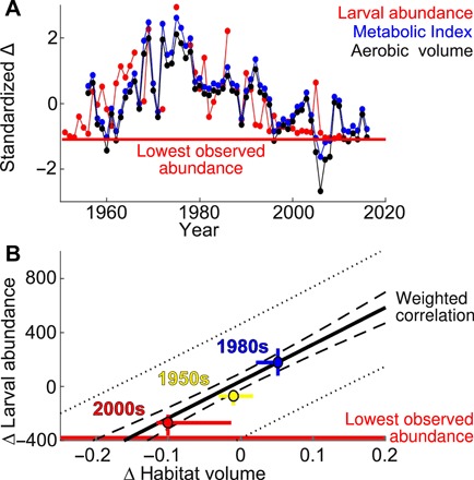
(A) For the SCB, standardized anomalies (Δ) in time of spawning season anchovy larval abundance are correlated with annual Φ and aerobic habitat volume predicted by the distribution-inferred ecophysiotype (lines between consecutive annual data). (B) Relationship between larval abundance and aerobically suitable habitat volume (fraction of upper 100 m), from the weighted mean response across ecophysiotypes (both normalized to CalCOFI 1956–2011 mean; dashed line is 95% confidence interval for the slope, dotted line is 95% prediction interval for annual values). Median spawning season abundance was 379.1 larvae dm⁻² (1956–2011), and dropped to historically low levels (1.9 larvae dm⁻²; red line) with a 15% decrease in aerobic habitat volume. Decadal means (filled circles) align closely with the slope derived from the interannual data (bars show the interannual range for each decade).

Across potential traits, changes in aerobic habitat could account for up to 75% of the time variance in anchovy abundance from 1956–2011 on decadal scales (10-year moving average; decadal differences in the spatial distributions of larvae are plotted in fig. S5). When interannual fluctuations are included (1-year moving average), the covariance decreases to 35 to 40%, in part because changes in habitat volume and larval abundance become decorrelated (noisy) when larval abundance bottoms out at historically low levels at either end of the time series. However, interannual variability also includes processes (e.g., larval cohort recruitment and El Niño) that may be less relevant to the species’ success on the climatic scales of interest here.

The distribution and time series analyses place independent but convergent constraints on the likely ecophysiotype for northern anchovy. We weight and combine the results of these approaches to determine likely ecophysiotypes (see the Supplementary Materials) and evaluate the response of anchovy larval abundance to aerobic habitat volume in the SCB; this sensitivity was tightly constrained (Fig. 4B)—a 15% (95% confidence interval, 12 to 20%) decrease in annual mean habitat volume relative to the CalCOFI historical mean corresponded with as low a larval abundance as ever observed in the SCB during the spawning season (1.9 larvae dm⁻², 0.5% of the median over the time series). Aerobic habitat decreases of this magnitude have occurred in the recent historical record and are similar to the range of interdecadal variability (Fig. 4B).

This apparent lower limit of larval abundance represents an observed population scale threshold; recent years with similarly, historically low larval abundance are associated with indicators of anchovy population declines in the southern CCS, including spawning collapses, reduced fisheries catches, reduced dietary fraction of anchovy in predators, and poor reproduction and increased mortality of anchovy predators [(12), and references therein]. To the degree that the anchovy population in the SCB is representative of the CCS as a whole, the associated aerobic habitat threshold defines a southern, ecologically-defined range limit, beyond which ecological disruption is likely (12). This occurs at a higher Φ than the more restrictive physiologically-defined range limit (where Φ < Φ_crit).

The distributions of northern anchovy are highly coherent with the long-term mean, interdecadal variability, and seasonal changes of aerobically suitable habitat—temperature-dependent hypoxia can predict these changes, which are not consistent with changing O₂, temperature, or primary productivity considered individually. To the degree that aerobic suitability actually underpins habitat constraints for anchovy, we can use historical population responses to identify critical ecological thresholds and project species aerobic habitat loss due to future climate change in the CCS.

Future anchovy habitat compression in the CCS

Over the next century, ocean warming and O₂ loss are expected to strongly reduce Φ in the North Pacific and the CCS [(8); fig. S7]. Thus, we anticipate that northern anchovy are vulnerable to aerobic habitat compression across their range with continued climate change. We used the likely anchovy physiological traits to predict aerobic habitat loss across the CCS by 2100 (Fig. 5 and fig. S8) under the “business as usual” greenhouse gas emission scenario (Representative Concentration Pathway 8.5) based on high-resolution regional downscaling of global climate projections. Across the downscaled climate models, both temperature (21 to 25% increase) and O₂ (9 to 13% decrease) change significantly and similarly from 2000 to 2100 over the coastal CCS (see the Supplementary Materials). Therefore we present aerobic habitat resulting from the ensemble mean forecasts of O₂ and temperature.

Fig. 5. Projected anchovy range contraction due to aerobic habitat loss.

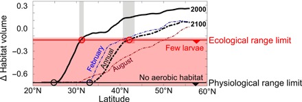
Aerobic habitat volume is computed at each latitude under historical climate (1995–2010; black line) and future climate (2100; dashed lines), and normalized by the mean value in the SCB. Thresholds for potential extirpation are defined using an ecological criterion (historically low larval abundance in the SCB; flat red line) and a more stringent physiological criterion (zero aerobic habitat in the SCB; flat black line). Latitudinal range limits are denoted by circles at the intersection of these extirpation thresholds with the computed habitat volume in each period. The 95% confidence intervals based on Fig. 4B are marked with gray bars.

We projected future changes in the latitudinal limit of the anchovy range based on the two metrics identified above: The ecological limit of aerobic habitat associated with historically low larval abundance and other indicators of regional population collapse, and the physiological range limit beyond which no aerobic habitat would be available. Because adult anchovy are mobile and seem to avoid a degree of habitat limitation at smaller scales of space and time, we determined annual average range shifts by averaging conditions over regions of similar alongshore and offshore extent to the SCB observations used in the time series (270 km × 270 km).

From 2000 to 2100, 30% of northern anchovies’ current latitudinal range, from 25°N to 33°N, is expected to lose all aerobically suitable habitat (based on annual mean conditions; Fig. 5). In other words, by reducing Φ below Φ_crit, warming and deoxygenation would cause anchovies’ energetic demands to exceed environmental O₂ supply across most of the southern CCS, likely resulting in extirpation south of the SCB. In an additional 23% of the present anchovy range, aerobic habitat compression is projected to reach levels associated with critically low larval abundance in the SCB, potentially threatening anchovy populations south of 42°N (95% confidence interval, 41.7°N to 43.3°N, based on uncertainty in the relationship between larval abundance and aerobic habitat). This threshold for ecological disruption is 11° farther north than the equivalent range limit inferred for 1995–2010, 31°N (95% confidence interval, 30.7°N to 31.7°N; Fig. 5). These projected range shifts are qualitatively similar both across the range of likely ecophysiotypes and across the inter-model spread of O₂ and temperature changes (each spans a response range of a few percent).

In either historical or future periods, individuals would still be expected south of these inferred potential habitat limits seasonally. If the ecological range limit inferred from the SCB is not representative of the entire CCS anchovy population, anchovy might persist closer to the physiological range limit. In addition, time periods with more favorable conditions may also allow anchovy to extend their range; northern anchovy colonized the Gulf of California in the mid-1980s following La Niña conditions (32). However, on a long-term average basis, we project that northern anchovies will lose much of their aerobic habitat and that current climate trends will lead to near-complete loss of aerobic habitat and thus likely extirpation from the southern CCS within this century.

DISCUSSION

Our results strengthen and extend the growing body of evidence that temperature-dependent hypoxia plays a central role in marine species distributions (8) and their response to climate change (9). The long-term mean and seasonally variable distributions of anchovy in the CCS, as well as the decadal variability of anchovy larval abundance in the SCB, are all consistent with the same set of Metabolic Index traits, indicating that temperature-dependent hypoxia is likely an important constraint for this key CCS species. These results identify physiologically-dependent aerobic habitat change as a likely mechanism underlying correlations between northern anchovy, O₂, and decadal scale climate indices (24, 33, 34), and provide empirical support for species response to aerobic habitat compression (8). Here, we discuss the broader implications and current limitations of the Metabolic Index framework for understanding the response of the CCS ecosystem to climate change.

Historically, seasonal and climate variability in the CCS appear to have shaped habitat suitability for anchovy more strongly through changes in O₂ than through changes in primary productivity. In addition to moving offshore during seasonal upwelling, anchovy consistently increase their aerobic scope during spawning by moving offshore or deeper (25, 26, 31). These movements are the opposite of what would be expected if primary productivity was the key driver of seasonal anchovy distributions. Furthermore, primary productivity shifts in the CCS over recent decades were out of phase with the multidecadal fluctuations of O₂ and anchovy larval abundances, because observed fluctuations of O₂ were largely caused by water mass displacements that increased surface nutrient supply and primary productivity when O₂ was low (35). A stronger sensitivity to O₂ than to primary productivity is consistent with the previously observed positive correlations between abundance of a number of mesopelagic and epipelagic planktivores, including anchovy, with climate conditions that favor low rather than high productivity (24). In addition, such species are positively correlated with both their predators and taxa competing for similar food (24), and anchovy abundance in particular is not correlated with fishing pressure (12).

Thus, while variability in food supply or resource competition in space (e.g., with sardines) may alter the offshore extent of northern anchovy (30, 36, 37), we find that anchovy and many other ecophysiotypes likely have aerobic limitation of habitat in the coastal CCS. While productivity could become a stronger driver of future species habitat, climate models do not project a robust change in primary productivity in the coastal CCS, in contrast to the significant decreases in O₂ and increases in temperature consistently projected across climate models (fig. S7).

The intensity of future aerobic habitat compression will vary strongly among species with different hypoxia traits and vertical habitat zonation (Fig. 6). From 0 to 200 m depth, climate trends are expected to decrease habitat volume most severely for ecophysiotypes with low hypoxia tolerance and high temperature sensitivity (e.g., at lower than average A_o and greater than average E_o, >50% loss of aerobic habitat by 2100). Greater habitat loss at mid-depths (>50% loss for most known ecophysiotypes from 200 to 400 m) may drive some mesopelagic fish to shallower depths. At even greater depths, historical variability and future trends are both greatly muted.

Fig. 6. Projected aerobic habitat loss by 2100 for varied marine ecophysiotypes.

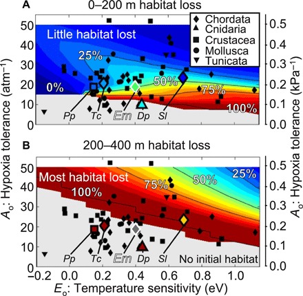
Relative habitat volume loss (2100–2000) across physiological traits (for assumed ratio of active to resting metabolic rates Φ_crit = 3.5) in the coastal CCS (27°N to 51°N, 0 to 200 m offshore; 12 km resolution ROMS with Representative Concentration Pathway 8.5 climate forcings). Percent habitat loss from (A) 0 to 200 m depth and (B) 200 to 400 m depth. Gray indicates no current aerobic habitat in the depth range. Known species traits are marked with black symbols for specific (sub)phyla (legend). Native CCS species are marked with open symbols, or, if the species-specific Φ_crit is known, with a larger marker and fill color corresponding to the species-specific aerobic habitat volume loss in the specified depth range. Lower Φ_crit results in higher aerobic habitat volume for the same physiological traits. The inferred anchovy ecophysiotype (assuming Φ_crit = 3.5 to translate A_o/Φ_crit onto plot) is marked with a large filled marker with white outline (Em, Engraulis mordax).

This differential severity of aerobic habitat compression across ecophysiotypes and vertical niches could lead to relative advantages for some species. In the CCS, the vertically migrating lampfish Stenobrachius leucopsarus show little decadal variation in historical larval abundance with interdecadal climate indices (38), consistent with expectations for their ecophysiotype (Fig. 2). Yet in the 200 to 400 m depth range near the base of their diel vertical migrations, where some climate sensitivity is expected (Fig. 6), such myctophid fishes have been shown to shoal along with low-O₂ conditions (39). Humboldt squid have behavioral and physiological adaptations to low-O₂ environments (40), which may have helped them benefit from vertical habitat compression of their myctophid prey (39).

The inferred sensitivity of anchovy to aerobic habitat may also underlie the striking oscillations between anchovy and sardine (33, 36). If anchovy are more hypoxia tolerant than sardine, as hypothesized in the Humboldt Current System (13, 41), this could help explain why anchovy sometimes outcompete sardine in the highly productive coastal zone while sardine are restricted to the lower primary productivity offshore. In this way, temperature-dependent hypoxia traits may contribute to observed offshore niche partitioning and the anti-correlated oscillations of anchovy and sardine that have long been observed.

Our results suggest that for mobile species like anchovy, offshore and regional migrations may be a preferred response to continued climate change. However, distribution changes due to habitat compression likely entail ecological trade-offs. For example, retreat from upwelling-driven hypoxia may limit food supply, and energetically costly spawning is already seasonally shifted in parts of the anchovy range (25, 31). Movement to better-ventilated surface waters may expose fish to greater predation (5, 12). These effects are implicitly accounted for in our ecological range limit projections based on historical thresholds, but may contribute to ecological disruption as aerobic habitat decreases over temporal and spatial scales that exceed the capacity of short-term migratory avoidance.

Over longer periods, physiological acclimation and evolutionary adaptation may also ameliorate some aerobic habitat loss. While northern anchovy maintain genetic similarity across their entire range over decadal time scales, they have slightly increased genetic diversity in the southern CCS (42). This increased diversity, and reduced body size, life span, and growth rate (25, 43, 44) in anchovy’s southernmost range could indicate acclimation or adaptation to lower O₂, although the physiological basis for this is debated (e.g., 45). However, if the large historical swings in aerobic habitat in the SCB were indeed a primary factor driving anchovy larval abundance, then the capacity to adapt or acclimate was apparently inadequate to sustain the demands of the local population.

The response of CCS ecosystems to climate change will be driven by physiological responses of individual species, but also modulated by ecological dynamics. Identifying species whose climate responses are mediated by simple and fundamental physiological constraints is a critical step in building an understanding of ecosystem behavior. Direct measurements of hypoxia traits coupled with long-term observations for interacting species provide a promising path to extending the Metabolic Index habitat framework to an ecosystem scale assessment of climate impacts.

MATERIALS AND METHODS

The observations, simulations, and analytical approaches used in this work are discussed here in sufficient detail to understand the analysis. Additional methodological details and caveats needed to reproduce the results are presented in the Supplementary Materials.

Data

Anchovy observational data

Anchovy observations were obtained from the Ocean Biogeographic Information System [OBIS; n = 1596; (21)] and from the National Oceanic and Atmospheric Administration West Coast groundfish bottom trawl survey [n = 373 after merging duplicate observations; (22)]. For mapping and evaluation of seasonal distributions offshore, we excluded eggs from the OBIS data (n = 52), leaving 1917 observations.

For the evaluation of anchovy-inhabited hydrographic conditions, we excluded observations that could not be accurately paired with either hydrographic observations or model output, leaving 1075 observations for this analysis (see the Supplementary Materials). Missing date information precluded the use of observations south of 32.63°N in the analysis (~6% of total observations that nonetheless covered nearly one-third of the historical anchovy range).

Larval abundance was obtained from the CalCOFI ichthyoplankton database (23) and binned by 1/3° latitude and longitude in space for the January to April peak spawning period (25, 31). A well-sampled subset of the CalCOFI stations (~75%) where anchovy larvae were often present (roughly 32°N to 35°N, and 0–270 km offshore, primarily in the SCB), was used for the time series analysis; this region is substantially similar to prior analyses of the CalCOFI icthyoplankton data [e.g., (6)]. Alternative binning approaches and potential data biases do not qualitatively change the results in this work. One year of the resulting larval time series (1987) was excluded from subsequent analysis because it was found to be an outlier (using either a generalized extreme studentized deviate test on the non-normal data or a Grubb’s test after Box-Cox transformation to a normal distribution).

Hydrographic observations and model simulations

Hydrographic data and resulting climatologies were obtained from the World Ocean Database (WOD) 2013 (46). Hydrographic data were spatially binned within the same region as the CalCOFI icthyoplankton data. Gaps in temperature and O₂ between sampled depths were filled via a moving mean interpolation with a window length of three observations for each cast. Resulting binned data were averaged seasonally and then annually to compensate for sampling biases (5, 6).

We used a regional model of the CCS circulation (ROMS) with a Biogeochemical Elemental Cycling model to hindcast physical and biogeochemical variables over the years 1995–2010 (15–18). The hydrographic variability was extended further back in time by combining high-resolution model fields with long-term, lower-resolution hydrographic observations starting in 1956.

The future (100-year) changes of hydrographic variables were derived from Coupled Model Intercomparison Project Phase 5 Representative Concentration Pathway 8.5 projections, dynamically downscaled within ROMS for evaluation of future CCS conditions. The Supplementary Materials contains an overview of the model configuration and validation, which are covered in detail in other work (15–18), and the specific earth system models and approach used in the dynamic downscalings. For the purposes of this work, the 100-year changes in temperature and O₂ were significant (P < 0.05) and consistent in the coastal CCS across the evaluated model forcings, justifying the use of ensemble-mean fields of hydrographic data to examine changes in aerobic habitat.

Statistical analyses

Anchovy spatial distribution analysis

The WOD data are generally too sparse to support pairing of hydrographic data to fish observations at better than 1° resolution and a monthly climatology for the entire multidecadal observation period; this spatial resolution does a poor job representing shoaling of isopycnal surfaces and hydrographic properties. The ROMS model is better suited to matching the scale and extent of anchovy observations, but the output must be corrected for the different mean conditions over the shorter model period and the longer WOD time series. Therefore, for each anchovy observation that could be paired with hydrographic data (n = 1075), we used the location and month of observation to find the closest ROMS 4 km resolution model cell. To compensate for density-dependent variation in hydrographic variables at a particular depth, the density coordinate of each observation was determined from WOD climatological fields interpolated to the ROMS model grid. Then, the climatological temperature and O₂ outputs from the model for the same density were assigned to each observation.

Because it is not possible to pair anchovy observations with precise hydrographic conditions from the historical, rather than climatological, conditions across the CCS, we also assigned observations to the month before and after each sample (i.e., a 3-month seasonal range of temperature and O₂ was used) to incorporate the variable range of conditions likely to encompass the true in situ conditions associated with a particular anchovy observation.

We binned these paired hydrographic data by 0.1 atm (10 kPa) and 0.5°C to generate an O₂-temperature space encompassing the anchovy observation locations. The hypoxic boundary in O₂-temperature space between waters with and without reported anchovy occurrences can be described in terms of Metabolic Index parameters (see Results). To distinguish between more and less likely ecophysiotypes, we evaluated the F1 score based on the presence and absence of anchovy in O₂-temperature space above and below the hypoxic boundary predicted for any ecophysiotype. This metric allows us to optimize between ecophysiotypes that constrain too small an O₂-temperature space but maximize presence within that space and ecophysiotypes that hardly constrain habitat but contain all observations.

Larval time series analysis

We computed annual mean Φ from WOD observations for both the best-fit ecophysiotype from the spatial distribution analysis, and for all combinations of potential Metabolic Index traits. The hydrographic observations were too patchy in space to consistently calculate aerobic habitat volume, but mean Φ from the well-sampled SCB region used for the icthyoplankton data could be accurately assessed and was similar to that of the model output. To first order, changes in Φ were regionally coherent and approximately constant with depth over the upper 100 m; therefore, the model output was corrected for the small mean offset relative to the hydrographic data-derived Φ (−0.1). Then the explicitly known relationship between Φ and aerobic habitat volume for every ecophysiotype in ROMS (fig. S9) was used to project the change in habitat volume in the model for any change in Φ based on observed temperature and O₂ over the hydrographic time series.

Over the SCB study region, the correlation of annual mean Φ and resulting aerobic habitat (0 to 100 m depth, for every ecophysiotype) with spawning season anchovy larval abundance was calculated using a Model II linear regression. Prior to correlation, all three variables were standardized using the mean and standard deviation of the time series (for each ecophysiotype). Correlations of 5- and 10-year moving means of the variables were also evaluated; longer averaging periods highlight longer period fluctuations. Here, we present correlations from 5-year moving means (fig. S4) as a compromise between including too much noise (associated with data patchiness and interannual variability which may be unrelated to climate drivers) and smoothing over potentially environmentally significant subdecadal variability. The relative fraction of total variance that could be explained by each ecophysiotype (proportional to the squared correlation coefficients, r²) was consistent across the evaluated averaging periods.

Likely anchovy ecophysiological trait analysis

For the purpose of identifying the magnitude and associated uncertainty of aerobic habitat loss corresponding to a critically low threshold in larval abundance, we inferred the most likely physiological trait range for anchovy based on both the time series analysis and the adult range distribution. Specifically, we compared a cost function for each combination of Metabolic Index traits, the ecological hypoxia tolerance (A_o/Φ_crit) and temperature sensitivity (E_o), by determining a relative weighting for each ecophysiotype (W_e; see the Supplementary Materials) based on the larval-habitat volume r² and the F1 scores from the bounded O₂-temperature space (both standardized relative to the mean and standard deviation of all evaluated ecophysiotypes). Higher than average r² and F1 scores were weighted more strongly, while lower than average anomalies were given negative weights, which reduce W_e. Ecophysiotypes for which either the null hypothesis of no time series correlation could not be rejected (α = 0.05, P > 0.05 for two-sided significance test) or the F1 score was equal to zero were assigned zero weight. We additionally weighted the result of the spatial distribution analysis twice as much as that of the time series analysis, as anchovy distribution is potentially more directly linked to adult anchovy ecophysiological constraints than the larval time series (however this weighting has a small effect on the results because of the strong correspondence between the results of the two independent methods).

No single ecophysiotype has markedly higher weight than all others, although we identify the single likeliest parameter combination (temperature sensitivity E_o = 0.4 eV or 6 × 10⁻²⁰ J, ecological hypoxia tolerance A_o/Φ_crit = 5.4 atm⁻¹ or 0.053 kPa⁻¹) for the purpose of mapping habitat changes. A compact range of Metabolic Index traits that has high cumulative weights and is expected to contain the true anchovy traits could nonetheless be identified (e.g., fig. S4). The Supplementary Materials include additional details regarding the environmental bounds on these traits and range of likely Metabolic Index parameters for anchovy. For the further determination of the weighted mean response of anchovy larval abundance to changing aerobic habitat volume, we excluded the 50% of lowest weight ecophysiotypes—ecophysiotypes with lower than average values of both r² and F1 scores, which show little skill at predicting anchovy response and presence and are unlikely to include the true anchovy ecophysiotype. We used W_e for the remaining ecophysiotypes for a weighted, linear-bisquare regression of anchovy larval abundance on the weighted-mean relative habitat volume change. This choice makes the weighted-mean response of anchovy to habitat loss more closely aligned with the relatively few, clustered ecophysiotypes with high weights. Other weighting choices are possible, but in general this 50% W_e is a simple way to focus our predictions around the ecophysiotypes most congruent with the available data instead of the large range of evaluated traits with very low predictive power.

SUPPLEMENTARY MATERIALS

Supplementary material for this article is available at http://advances.sciencemag.org/cgi/content/full/6/20/eaay3188/DC1

REFERENCES AND NOTES

- 1.IPCC, Climate Change 2014: Impacts, Adaptation, and Vulnerability. Part A: Global and Sectoral Aspects. Contribution of Working Group II to the Fifth Assessment Report of the IPCC (Cambridge Univ. Press, 2014), 1132 pp. [Google Scholar]
- 2.Long M. C., Deutsch C., Ito T., Finding forced trends in oceanic oxygen. Global Biogeochem. Cycles 30, 381–397 (2016). [Google Scholar]
- 3.Northwest Fisheries Science Center, Ecosystem status report of the California Current for 2017: A summary of ecosystem indicators compiled by the California Current Integrated Ecosystem Assessment Team (CCIEA) (NOAA Technical Memorandum NMFS-NWFSC, NOAA, 2017); 10.7289/V5/TM-NWFSC-139. [DOI]
- 4.Di Lorenzo E., Combes V., Keister J. E., Strub P. T., Thomas A. C., Franks P. J. S., Ohman M. D., Furtado J. C., Bracco A., Bograd S. J., Peterson W. T., Schwing F. B., Chiba S., Taguchi B., Hormazabal S., Parada C., Synthesis of Pacific Ocean climate and ecosystem dynamics. Oceanography 26, 68–81 (2013). [Google Scholar]
- 5.Koslow J. A., Goericke R., Lara-Lopez A., Watson W., Impact of declining intermediate-water oxygen on deepwater fishes in the California Current. Mar. Ecol. Prog. Ser. 436, 207–218 (2011). [Google Scholar]
- 6.Koslow J. A., Goericke R., Watson W., Fish assemblages in the Southern California Current: Relationships with climate, 1951-2008. Fish. Oceanogr. 22, 207–219 (2013). [Google Scholar]
- 7.Keller A. A., Ciannelli L., Wakefield W. W., Simon V., Barth J. A., Pierce S. D., Species-specific responses of demersal fishes to near-bottom oxygen levels within the California Current large marine ecosystem. Mar. Ecol. Prog. Ser. 568, 151–173 (2017). [Google Scholar]
- 8.Deutsch C., Ferrel A., Seibel B., Pörtner H.-O., Huey R. B., Climate change tightens a metabolic constraint on marine habitats. Science 348, 1132–1135 (2015). [DOI] [PubMed] [Google Scholar]
- 9.Penn J. L., Deutsch C., Payne J. L., Sperling E. A., Temperature-dependent hypoxia explains biogeography and severity of end-Permian marine mass extinction. Science 362, eaat1327 (2018). [DOI] [PubMed] [Google Scholar]
- 10.Pörtner H.-O., Knust R., Climate change affects marine fishes through the oxygen limitation of thermal tolerance. Science 315, 95–97 (2007). [DOI] [PubMed] [Google Scholar]
- 11.Peterson C. C., Nagy K. A., Diamond J., Sustained metabolic scope. Proc. Natl. Acad. Sci. U.S.A. 87, 2324–2328 (1990). [DOI] [PMC free article] [PubMed] [Google Scholar]
- 12.MacCall A. D., Sydeman W. J., Davison P. C., Thayer J. A., Recent collapse of northern anchovy biomass off California. Fish. Res. 175, 87–94 (2016). [Google Scholar]
- 13.Bertrand A., Chaigneau A., Peraltilla S., Ledesma J., Graco M., Monetti F., Chavez F. P., Oxygen: A fundamental property regulating pelagic ecosystem structure in the coastal Southeastern Tropical Pacific. PLOS ONE 6, e29558 (2011). [DOI] [PMC free article] [PubMed] [Google Scholar]
- 14.Perry A. L., Low P. J., Ellis J. R., Reynolds J. D., Climate change and distribution shifts in marine fishes. Science 308, 1912–1915 (2005). [DOI] [PubMed] [Google Scholar]
- 15.Renault L., Deutsch C., McWilliams J. C., Frenzel H., Liang J.-H., Colas F., Partial decoupling of primary productivity from upwelling in the California Current system. Nat. Geosci. 9, 505–508 (2016). [Google Scholar]
- 16.Durski S. M., Barth J. A., McWilliams J. C., Frenzel H., Deutsch C., The influence of variable slope-water characteristics on dissolved oxygen levels in the northern California Current System JGR. Oceans 122, 7674–7697 (2017). [Google Scholar]
- 17.C. Deutsch, H. Frenzel, James C. Mc Williams, L. Renault, F. Kessouri, E. Howard, J.-H. Liang, D. Bianchi, S. Yang, Biogeochemical variability in the California Current System. bioRxiv 942565 [Preprint]. 11 February 2020. 10.1101/2020.02.10.942565. [DOI]
- 18.L. Renault, J. C. McWilliams, A. Jousse, C. Deutsch, H. Frenzel, F. Kessouri, The physical structure and behavior of the california current system. bioRxiv 942730 [Preprint]. 12 February 2020. 10.1101/2020.02.10.942730. [DOI]
- 19.Meyers R. A., When do environment-recruitment correlations work? Rev. Fish Biol. Fisheries 8, 285–305 (1998). [Google Scholar]
- 20.Beale C. M., Lennon J. J., Gimona A., Opening the climate envelope reveals no macroscale associations with climate in European birds. Proc. Natl. Acad. Sci. U.S.A. 105, 14908–14912 (2008). [DOI] [PMC free article] [PubMed] [Google Scholar]
- 21.OBIS and data contributors, Distribution records of Engraulis mordax (Girard 1854), and other species, 1953–2015. OBIS data server (2019); http://iobis.org/.
- 22.National Oceanic and Atmospheric Administration Northwest Fishery Science Center, Trawling records of Engraulis mordax from West Coast groundfish bottom trawl surveys. NWFSC Fishery Resource Analysis and Monitoring Data Warehouse (2019); https://www.nwfsc.noaa.gov/data/.
- 23.CalCOFI and data contributors, CalCOFI icthyoplankton database, 1951–2011. NOAA ERDDAP data server (2016); https://coastwatch.pfeg.noaa.gov/erddap.
- 24.Koslow J. A., Davison P., Lara-Lopez A., Ohman M. D., Epipelagic and mesopelagic fishes in the southern California Current System: Ecological interactions and oceanographic influences on their abundance. J. Mar. Syst. 138, 20–28 (2014). [Google Scholar]
- 25.Mais K. F., Pelagic fish surveys in the California Current. Cal. Fish Game Fish. Bull. 162, 1–79 (1974). [Google Scholar]
- 26.Laroche J. L., Richardson S. L., Reproduction of northern anchovy, Engraulis mordax, off Oregon and Washington. NOAA Fish. Bull. 78, 603–618 (1980). [Google Scholar]
- 27.Di Lorenzo E., Seasonal dynamics of the surface circulation in the Southern California Current System. Deep Sea Res. Part II Top Stud. Oceanogr. 50, 2371–2388 (2003). [Google Scholar]
- 28.Munro D. R., Quay P. D., Juranek L. W., Goericke R., Biological production rates off the Southern California coast estimated from triple O2 isotopes and O2: Ar gas ratios. Limnol. Oceanogr. 58, 1312–1328 (2013). [Google Scholar]
- 29.Haugen C. W., Messersmith J. D., Wickwire R. H., Progress report on anchovy tagging off California and Baja California, March 1966 through May 1969. Cal. Fish Game Fish. Bull. 147, 75–89 (1969). [Google Scholar]
- 30.Fiechter J., Rose K. A., Curchitser E. N., Hedstrom K. S., The role of environmental controls in determining sardine and anchovy population cycles in the California Current: Analysis of an end-to-end model. Prog. Oceanogr. 138, 381–398 (2015). [Google Scholar]
- 31.Methot R. D., Synthetic estimates of historical abundance and mortality for northern anchovy. Am. Fish. Soc. Sym. 6, 66–82 (1989). [Google Scholar]
- 32.Hammann M. G., Cisneros-Mata M. A., Range extension and commercial capture of the northern anchovy, Engraulis mordax Girard, in the Gulf of California, Mexico. Cal Fish Game 75, 49–53 (1989). [Google Scholar]
- 33.Chavez F. P., Ryan J., Lluch-Cota S. E., Ñiquen M., From anchovies to sardines and back: Multidecadal change in the Pacific Ocean. Science 299, 217–221 (2003). [DOI] [PubMed] [Google Scholar]
- 34.Lindegren M., Checkley D. M. Jr., Rouyer T., MacCall A. D., Stenseth N. C., Climate, fishing, and fluctuations of sardine and anchovy in the California Current. Proc. Natl. Acad. Sci. U.S.A. 110, 13672–13677 (2013). [DOI] [PMC free article] [PubMed] [Google Scholar]
- 35.Deutsch C., Brix H., Ito T., Frenzel H., Thompson L., Climate-forced variability of ocean hypoxia. Science 333, 336–339 (2011). [DOI] [PubMed] [Google Scholar]
- 36.Checkley D. M. Jr., Asch R. G., Rykaczewski R. R., Climate, anchovy, and sardine. Ann. Rev. Mar. Sci. 9, 469–493 (2017). [DOI] [PubMed] [Google Scholar]
- 37.Robinson K. L., Ruzicka J. J., Decker M. B., Brodeur R. D., Hernandez F. J., Quiñones J., Acha E. M., Uye S.-i., Mianzan H., Graham W. M., Jellyfish, forage fish, and the world’s major fisheries. Oceanography 27, 104–115 (2014). [Google Scholar]
- 38.Hsieh C.-H., Reiss C., Watson W., Allen M. J., Hunter J. R., Lea R. N., Rosenblatt R. H., Smith P. E., Sugihara G., A comparison of long-term trends and variability in populations of larvae of exploited and unexploited fishes in the Southern California region: A community approach. Prog. Oceanogr. 67, 160–185 (2005). [Google Scholar]
- 39.Stewart J. S., Hazen E. L., Bograd S. J., Byrnes J. E. K., Foley D. G., Gilly W. F., Robison B. H., Field J. C., Combined climate- and prey-mediated range expansion of Humboldt squid (Dosidicus gigas), a large marine predator in the California Current System. Glob. Chang. Biol. 20, 1832–1843 (2014). [DOI] [PubMed] [Google Scholar]
- 40.Seibel B. A., Hafker N. S., Trubenbach K., Zhang J., Tessier S. N., Pörtner H. O., Rosa R., Storey K. B., Metabolic suppression during protracted exposure to hypoxia in the jumbo squid, Dosidicus gigas, living in an oxygen minimum zone. J. Exp. Biol. 217, 2555–2568 (2014). [DOI] [PubMed] [Google Scholar]
- 41.Salvatteci R., Field D., Gutiérrez D., Baumgartner T., Ferreira V., Ortlieb L., Sifeddine A., Grados D., Bertrand A., Multifarious anchovy and sardine regimes in the Humboldt Current System during the last 150 years. Glob. Chang. Biol. 24, 1055–1068 (2018). [DOI] [PubMed] [Google Scholar]
- 42.LeComte F., Grant W. S., Dodson J. J., Rodriguez-Sanchez R., Bowen B. W., Living with uncertainty: Genetic imprints of climate shifts in East Pacific anchovy (Engraulis mordax) and sardine (Sardinops sagax). Mol. Ecol. 13, 2169–2182 (2004). [DOI] [PubMed] [Google Scholar]
- 43.Vrooman A. M., Paloma P. A., Zweifel J. R., Electrophoretic, morphometric, and meristic studies of subpopulations of northern anchovy, Engraulis mordax. Cal. Fish Game 67, 39–51 (1981). [Google Scholar]
- 44.Parrish R. H., Mallicoate D. L., Mais K. F., Regional variations in the growth and age composition of northern anchovy, Engraulis mordax. Fish. Bull. 83, 483–496 (1985). [Google Scholar]
- 45.Audzijonyte A., Barneche D. R., Baudron A. R., Belmaker J., Clark T. D., Marshal C. T., Morrongiello J. R., van Rijn I., Is oxygen limitation in warming waters a valid mechanism toexplain decreased body sizes in aquatic ecosystems? Glob. Ecol. Biogeogr. 28, 64–77 (2018). [Google Scholar]
- 46.T. P. Boyer, J. I. Antonov, O. K. Baranova, C. Coleman, H. E. Garcia , A. Grodsky, R. A. Johnson, D. R. Locarnini, A. V. Mishonov, T. D. O'Brien, C. R. Paver, J. R. Reagan, D. Seidov, I. V. Smolyar, M. M. Zweng, World Ocean Database 2013. NOAA Atlas NESDIS 72 (2013); http://hdl.handle.net/11329/357.
- 47.Moore J. K., Doney S. C., Kleypas J. A., Glover D. M., Fung I. Y., An intermediate complexity marine ecosystem model for the global domain. Deep Sea Res. Part II Top Stud. Oceanogr. 49, 403–462 (2002). [Google Scholar]
- 48.Taylor K. E., Stouffer R. J., Meehl G. A., An overview of CMIP5 and the experiment design. Bull. Am. Meteorol. Soc. 93, 485–498 (2012). [Google Scholar]
- 49.Goute C., Gaussier E., A probabilistic interpretation of precision, recall and F-score, with implication for evaluation. Adv. Inform. Retriev. 3408, 345–359 (2005). [Google Scholar]
- 50.A. Trujillo-Ortiz, R. Hernandez-Walls, gmregress: Geometric Mean Regression (Reduced Major Axis Regression) MATLAB file (2010); http://www.mathworks.com/matlabcentral/fileexchange/27918-gmregress.
Associated Data
This section collects any data citations, data availability statements, or supplementary materials included in this article.