Greening and legume-supported crop rotations: An impacts assessment on Italian arable farms

Abstract

Since the 1990s, the European Union has progressively and structurally reformed the Common Agricultural Policy with a gradual integration of environmental objectives. For the period post-2020, one of the most relevant changes could be the upgrading of the crops diversification, imposing it as an obligation to rotate crops by introducing legumes in the cropping patterns. This paper proposes an assessment of the possible effects of such obligation on the arable crops sector in Italy.

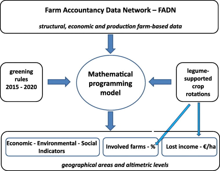
The analysis uses a mathematical programming model calibrated and validated by way positive approach and is conducted on data of about 2800 Italian farms of the Farm Accountancy Data Network. Moreover, the analysis is structured by geographical area and altimetric level in order to consider typical specificities of Italian farms according to their localization.

Our results show the legume-supported crop rotations reduce the general environmental pressure of agricultural activities and affect a large part of the arable land, against reduced economic impacts. In the majority of farms the lost income per hectare is lower than the national average value of the decoupled payments. Yet, the legume-supported crop rotations determine a reduction in the production of main crops and, especially in some areas, negative economic and social impacts.

All this suggests that the legume-supported crop rotations are an opportunity to adopting sustainable agricultural practices and that Member States could implement the agronomic practice differently for areas and use additional instruments to meet the EU's objectives. Especially the decoupled and coupled payments are needed to limit economic losses and incentivize farmers towards virtuous behaviour.

Graphical abstract

Highlights

• •Sustainability implications of agricultural land use and land use change
• •Legume-supported crop rotations reduces the environmental pressures
• •Lost income lower than national levels of decoupled payments
• •Efficient market mechanisms and coupled payments to support farms' profitability
• •Reductions of the main crops and possible imports from other countries

1. Introduction

Since the 1990s, the European Union (EU) has progressively and structurally reformed the Common Agricultural Policy (CAP) with a gradual integration of environmental objectives and motivations into the CAP (Allen and Hart, 2013). The last CAP reform, started in 2015, introduced the greening criteria that conditioned 30% of direct payments to meet three environmental requirements: crop diversification, maintaining permanent grassland and Ecological Focus Area (Matthews, 2013; Alons, 2017). The European Commission (EC) proposed to reform the green architecture of the Common Agricultural Policy (CAP) post 2020 in such a way as to increase the level of environmental and climate ambition (European Commission, 2017a, European Commission, 2017b, European Commission, 2018). As regards the greening, the EC considers the crop diversification is not sufficient to improve the environmental performance and long-term viability of European arable crops systems, and proposes to introduce a sustainable rotation of agricultural crops, in particular with legumes. Furthermore, Member States should define the new rules and standards of the agricultural policy taking into account specific characteristics of their territories, including soil and climatic condition, existing farming systems, land use, crop rotation, farming practices, and farm structures (European Commission, 2018).

The CAP's integration of more environmental concerns has increased the demand for tools to help assess the impact of decisions on agriculture and on its economic and physical environment (Gohin, 2006; Balkhausen et al., 2007; Dessart et al., 2019). Economic models can provide these types of evaluation using available agricultural information for the entire EU, such as the data provide by the Farm Accountancy Data Network (FADN). Specifically, the micro-economic approach of mathematical programming models allows the technical aspects of agricultural production to be taken into account (Godard et al., 2008). Within the current agricultural economics mathematical programming toolkit, two main types of programming models can be distinguished: Normative Mathematical Programming (NMP) and Positive Mathematical Programming (PMP). This latter type calibrates mathematical programming models to observed behaviour during a reference period using the information provided by the dual variables of the calibration constraints (Howitt, 1995; Arfini and Paris, 1995; Paris and Howitt, 1998; de Frahan et al., 2016). Many analyses of the impact of farm policy reforms have been conducted using mathematical programming models in order to identify the possible solutions of crop-mix and to carry out sustainability analysis (Balezentis et al., 2020), also in the context of introducing legumes into cropping systems (Preissel et al., 2017).

In this research context, the main objective of this study is to evaluate the possible impact of legume-supported crop rotations in the arable crops sector in Italy. The analysis uses a mathematical programming model calibrated and validated by way positive approach (PMP) and is conducted on data of about 2800 Italian farms of the FADN database. Moreover, the analysis is structured by geographical area and altimetric level in order to capture typical specificities of Italian farms according to their localization. The impacts are evaluated in terms of land use and of economic, environmental and social indicators, such as the gross income, the use of water, chemical inputs, and labour. The results are shown and discussed both nationally and by geographic area and altimetric levels. The analysis also evaluates the lost income resulting from the obligation of legume-supported crop rotation, compared with the average national values of decoupled payments. This allows to analyse the effectiveness of decoupled payments in stimulating the compliance of environmental rules and then virtuous behaviour by farmers.

The paper is structured as follows. The next section on Materials and Methods describes the sample of farms, the main changes made to greening and the economic model used in the analysis. After the description and the Discussion of the Results, some policy suggestions are provided in the Conclusions. The paper ends with the discussion of limits and possible developments.

2. Materials and methods

2.1. Characteristics of farms sample

The analysis was carried out on a FADN sample of Italian farms. The FADN provides data for evaluating the income of agricultural holdings and the impacts of the Common Agricultural Policy. The data refer to physical and structural characteristic (such as location, crop areas, labour force, uses of chemical input and water, etc.) and economic data (such as the revenue of the different crops, production costs, CAP payments, etc.).1

The farms sample includes 2798 farms belonging to the following Types of Farming (TF): TF15-Specialist cereals, oilseeds and protein crops, TF16-General field cropping and TF22-Specialist horticulture outdoor, which are the most influenced by the greening practices, including the crop rotations. The selected farms represent 147,603 Italian farms and 3591,000 ha of Utilized Agricultural Area (Table 1 ).

Table 1.

Characteristics of the farms sample: number, land use and environmental, social, economic indicators. Absolute value for total Italy and percentage for geographical area and altimetric level (year 2014).

	Total	North	Central	South	Plain	Hill	Mountain
Representative farms (n°)	147,603	42.5	15.7	41.7	49.6	37.8	12.6
UAA (kha)	3591	46.6	17.7	35.7	52.3	37.5	10.2
Land use (kha)
Main crops
durum wheat	807	6.4	26.4	67.2	27.7	59.1	13.2
maize	472	95.7	2.7	1.6	86.2	12.8	1.0
soft wheat	326	80.2	13.9	5.9	69.6	25.5	4.9
barley	117	27.9	21.2	50.9	32.9	55.0	12.1
processed tomato	80	43.4	10.2	46.4	84.1	12.8	3.0
Legumes crops
alfalfa	235	69.9	24.0	6.2	50.8	38.3	10.9
leguminous herbage	196	1.6	19.0	79.4	11.6	56.0	32.4
soybean	154	99.5	0.3	0.2	90.4	9.6	0.0
faba bean	83	0.1	17.4	82.5	29.9	58.2	11.9
Others	1122	46.4	20.0	33.6	54.4	34.7	10.9
Indicators (MM)
Gross margin - €	5023	49.9	13.9	36.2	63.2	29.7	7.1
Water - m3	2878	67.6	2.1	30.2	89.8	8.7	1.5
Nitrogen - kg	327	55.6	18.4	25.9	64.2	30.8	5.0
Phosphorus - kg	131	45.0	13.7	41.4	58.5	35.1	6.4
Potassium - kg	102	63.9	10.6	25.5	73.8	19.6	6.6
Labour - h	215	31.3	15.3	53.4	54.6	35.7	9.7

The farms are located in the following way: 42.5% North, 15.7% Centre and 41.8% South; 49.6% Plain, 37.8% Hill and 12.6% Mountain.

The most cultivated crop is durum wheat, mainly in hill (59.1%) and in the Centre (26.4%) and South of Italy (67.2%). Maize is grown mainly in the northern Italy (95.7%) and in plain (86.2%). Soft wheat is cultivated mainly in the northern Italy (80.2%) while barley in southern Italy (50.9%). Finally, the processed tomato is grown mainly in plain (84.1%), in the southern Italy (46.4%) and in the northern Italy (43.4%). Overall, the sum of these five crops is about 1800 ha.

As for forage legumes, alfalfa is grown mainly in northern Italy (69.9%) and then in central Italy (24.0%), while the leguminous herbage in southern Italy (79.4%). Regarding the grain legumes, soybean is cultivated in the northern Italy (99.5), and the faba bean in the southern Italy (82.5%) and then in central Italy (17.4%). The total area devoted to legumes crops is about 670 ha. Therefore, the ratio between the legumes crops and main crops is around 37%.

In terms of economic results, 50% of the total gross margin of the sector is produced in northern Italy where, as seen previously, a large part of the farms and the production of high-income crops (maize, soya and rice) are localized.

Regarding the use of inputs, 89.8% of irrigation water is used in plain, 67.6% in the northern Italy and 30.2% in the southern Italy. As regards of nitrogen, making the comparison with the percentages of UAA, the use is particularly intensive in the northern Italy and in plain areas. Interestingly, 53.4% of the total hours agricultural labour is employed in southern Italy.

2.2. First pillar of the CAP: cross-compliance, greening and crop rotations

The CAP is currently organized into two pillars, with the first related to direct payments and Common Market Organizations (CMOs) and the second related to rural development policy. The first pillar is the most important in financial terms and, currently, the direct payments include decoupled payments (basic and greening) and coupled payments. Moreover, two types of environmental tools are planned in the first pillar of CAP: cross-compliance and greening.

Cross-compliance is a system of linkage between area (and animal) based direct payments and a range of obligations. These obligations originate in CAP legislation, in the case of standards for Good Agricultural and Environmental Condition (GAEC), or in non-CAP directives and regulations, in the case of Statutory Management Requirements (SMRs). All the GAEC standards and some of the SMRs are environmental concerning climate change, water, soil, biodiversity and landscape. If the farmers do not meet these obligations, the direct payments may be reduced.

Greening requires compliance with three practices concerning crop diversification, maintenance of permanent grassland and the presence of an Ecological Focus Areas (EFA). Crop diversification requires the presence of more crops in farms where the arable land exceeds 10 ha: the main crop cannot exceed 75% of the arable land; at least three crops for farms that exceed 30 ha and the third crop must be at least equal to 5% of the arable land.

In the CAP post 2020, the new green architecture will effectively merge and streamline the two elements in the current CAP (cross-compliance and greening), trying to draw on the content and strengths of the current systems and make some improvements. One of the main changes regards the crop diversification whose current requirement (the presence of more than one crop on the arable land of a farm at any one time) will be upgraded to an obligation of crop rotation, especially with legumes crops. This requirement will be framed within the Good Agricultural and Environmental Condition, in the Soil Protection and Quality section. (European Commission, 2018).

2.3. Simulated scenarios and PMP model

The Positive Mathematical Programming model was calibrated to the scenario observed in 2014 year. This year is fundamental to conduct the analysis because represents the possible “monoculture or few crops” situation, that is, before the introduction of greening and related diversification practices. The 2014 scenario allows to isolate the impact of the changes of greening application, to calculate the lost income respect a scenario without the environmental rules and the comparison with the decoupled payments.

A first simulation of the model concerned the application of the greening rules currently in use, including these defined in the recent Omnibus regulation (Cortignani and Dono, 2019), in order to obtain a baseline that represents the current situation in terms of greening application. Following, additional simulations on legume-supported crop rotation applicable in the CAP post 2020 were carried out, as shown in the Table 2 .

Table 2.

Simulated scenarios on different ratios of legumes crops in the cropping patterns.

	Scenarios	Main crops	Legumes crops	T	Code name
2014		no constraints	no constraints	0	2014
greening 2015–2020		≤75%	no constraints	0	baseline
post 2020	continuous cropping 3 years	≤75%	≥ 25%	1/3	c_3y
	continuous cropping 2 years	≤67%	≥ 33%	1/2	c_2y
	3/5 rotation	≤60%	≥ 40%	2/3	3/5_rot
	biennial rotation	≤50%	≥ 50%	1	b_rot

The main arable crops (durum wheat, maize, soft wheat, barley, processed tomato) are subjected to different ratios with leguminous crops (forage and grain) in an increasingly stringent and binding manner. The first simulation (c_3y) requires that the main crop must be at most equal to 75% of the arable land (as required by the current diversification rule) and the remaining part (25%) must be composed of legumes crops. The other simulations (c_2y, 3/5_rot and b_rot) require increasingly stringent percentages as regards the main crops (67%, 60%, 50%) and therefore greater surfaces of legumes crops on the remaining part. Therefore, compared to the diversification rules currently in force, the first simulation determine changes on the remaining part of the surface (25%), while the others influence also the surfaces devoted to main crops. In particular the last simulation conducted (b_rot) seems unlikely considering that the “rotation practice” should be included in the new rules of cross-compliance. However, this simulation was considered in the analysis in order to evaluate the lost income of more extreme scenarios.

The standard representation of production choices considering different ratios of legumes in the cropping patterns can be described by the following quadratic programming model, where the n set denotes the farms and the j index denotes the crops2 :

$$\underset{x_{n,j}}{max}z=\sum _{\mathrm{n},j}\left(P_{n,j}\ast Y_{n,j}+{\mathit{CP}}_{n,j}-{\mathit{AC}}_{n,j}\left(x_{n,j}\right)\right)\ast x_{n,j}+\left({\mathit{VEb}}_n+{\mathit{VEg}}_n\right)\ast {\mathit{NE}}_n$$

$$s.\mathit{to}$$

$$\sum _{\mathrm{j}}{\mathrm{x}}_{\mathrm{n},\mathrm{j}}\le {\mathrm{Bld}}_{\mathrm{n}}\forall \mathrm{n}$$

$$\sum _{\mathrm{j}}{\mathrm{Alb}}_{\mathrm{n},\mathrm{j}}\ast {\mathrm{x}}_{\mathrm{n},\mathrm{j}}\le {\mathrm{Blb}}_{\mathrm{n}}\forall \mathrm{n}$$

$$\mathrm{T}\ast {\mathrm{x}}_{\mathrm{n},\text{jmain}}\le \sum _{\text{jlegumes}}{\mathrm{x}}_{\mathrm{n},\text{jlegumes}}\forall \mathrm{n},\text{jmain}$$

$${\mathrm{x}}_{\mathrm{n},\mathrm{j}}\ge 0\forall \mathrm{n},\mathrm{j}$$

where z denotes the objective function value; x _{n, j} represent the endogenous variables of the model (hectares allocated to crop j in each farm n); P _{n, j} and Y _{n, j} are, respectively, the prices and the yields per unit of activity; CP _{n, j} are CAP coupled payments (also provided for legume crops); AC _{n, j}(x _{n, j}) denotes average variable cost function per unit of activity (explained later); VEb _n and VEg _n are the unit value of entitlements (basic and greening); NE _n are the number of entitlements.

Bld _n is the land availability for each farm (n). Alb _{n, j} are the labour requirements of the various crops (j) and farms (n) and Blb _n is the labour availability for each farm (n).

T is a scalar term (with different values according to simulated scenarios, see Table 2) that multiples the main crops (jmain = durum wheat, maize, soft wheat, barley, processed tomato) subject to rotations by determining the ratio with all the legumes crops (jlegumes = forage and grain legumes). There are two possible way of implementing a crop rotation in the mathematical programming models (Hazell and Norton, 1986). One approach is to plant the entire farm to a single crop each year. In this case the same crop will only be grown again when its turn in the sequence arrives. This approach is not commonly practiced, particularly where special machines or equipment are required for individual crops, or where livestock are involved in the rotation. It is also a risky approach because the farmer is entirely dependent on the yield and price of a single crop each year. The second approach is to divide the farm into roughly equal parts, and to rotate the crops within each part in such a way that the total acreage of each crop grown on the farm is about constant each year. This is the practice followed by most farmers who adapt a rotation, and applied also in this analysis.

The average variable cost function per unit of activity, AC_n,j (x_n,j), has the following form:

$${\mathrm{AC}}_{\mathrm{n},\mathrm{j}}\left({\mathrm{x}}_{\mathrm{n},\mathrm{j}}\right)={\mathrm{\alpha }}_{\mathrm{n},\mathrm{j}}+\frac{1}{2}{\mathrm{\beta }}_{\mathrm{n},\mathrm{j}}\ast {\mathrm{x}}_{\mathrm{n},\mathrm{j}}$$

where

$${\mathrm{\alpha }}_{\mathrm{n},\mathrm{j}}={\mathrm{c}}_{\mathrm{n},\mathrm{j}}=\mathrm{c}\_{\text{seeds}}_{\mathrm{n},\mathrm{j}}+\mathrm{c}\_{\text{fertilisers}}_{\mathrm{n},\mathrm{j}}+\mathrm{c}\_{\text{pest}}_{\mathrm{n},\mathrm{j}}+\mathrm{c}\_{\text{other}}_{\mathrm{n},\mathrm{j}}$$

and

$${\mathrm{\beta }}_{\mathrm{n},\mathrm{j}}=\frac{{\mathrm{\mu }}_{\mathrm{n},\mathrm{j}}}{{\mathrm{x}}_{\mathrm{n},\mathrm{j}}^0}$$

The c _{n, j} are the observed accounting costs, i.e. seeds, fertilizers, pest management and other,3 where the first three types represent about 70% of the total accounting cost. The distinction could be fundamental to simulate variations of the c_fertilisers _{n, j} and c_pest _{n, j} in possible scenarios on benefits of crop rotations (not considered in this paper).

μ _{n, j} are the dual values determined by means of the calibration constraints used in the first phase of the PMP approach (Arfini and Paris, 1995; Howitt, 1995; Paris and Howitt, 1998; Heckelei and Wolff, 2003). This approach not only automatically and exactly calibrates the model to observed activity levels, but also avoids adding ad-hoc constraints and over-specialised responses of the model to policy changes (Heckelei et al., 2012; de Frahan, 2016).

3. Results

The used model allows to obtain different type of the results: land use changes, economic results, use of labour. Moreover, as seen in Table 1, the FADN data also provide indications about the uses of water and chemical inputs, for each crops, and consequently the land use changes in the simulation scenarios determine an impact of uses of these factors (water and chemicals).

The results concern the land use for the total area (Table 3 ), the value of various indicators such as gross margin, uses of water, chemical and labour by total area (Table 4 ) and by geographical area and altimetric level (Table 5 ), the involved farms and farm land, the lost income (Table 6 ), the lost income compared with average values of the decoupled payments (Table 7 ).

Table 3.

Land use in the baseline (absolute values in kha) and in the simulated scenarios (%Δ over baseline). Total area.

Crops	baseline	c_3y	c_2y	3/5_rot
Main crops	1659	−5.6	−10.4	−14.8
durum wheat	771	−5.0	−10.1	−15.0
maize	410	−5.9	−10.9	−15.5
soft wheat	289	−6.3	−10.3	−13.5
barley	100	−5.0	−8.8	−12.5
processed tomato	89	−7.8	−12.7	−17.0
Legumes crops	670	4.0	8.2	12.2
alfalfa	225	0.1	0.9	1.7
leguminous herbage	182	5.6	10.8	15.8
soya	176	5.6	10.8	15.9
faba bean	86	7.4	15.9	24.6
Others crops	1005	1.1	2.1	3.1

Table 4.

Economic, environmental and social indicators: absolute values (MM) in the baseline and percentage changes (%Δ over baseline) in the simulated scenarios. Total area.

	baseline	c_3y	c_2y	3/5_rot
Gross margin - €	4720.5	−0.8	−1.7	−2.4
Water - m3	2744.9	−2.8	−5.0	−6.9
Nitrogen - Kg	312.5	−2.6	−4.8	−6.8
Phosphorus - Kg	128.1	−2.1	−3.7	−5.1
Potassium - Kg	99.2	−2.0	−3.5	−4.7
Labour - h	209.9	−1.4	−2.3	−3.1

Table 5.

Economic, environmental and social indicators: absolute values (MM) in the baseline and percentage changes (%Δ over baseline) in the simulated scenarios. Geographical area and altimetric level.

		baseline	c_3y	c_2y	3/5_rot
Gross margin - €	North	2344.3	−1.0	−1.8	−2.6
	Central	670.0	−0.5	−1.0	−1.4
	South	1706.2	−0.6	−1.7	−2.6
	Plain	2947.2	−0.9	−1.8	−2.6
	Hill	1413.8	−0.6	−1.5	−2.3
	Mountain	359.5	−0.6	−1.2	−1.7
Water - m3	North	1889.9	−3.3	−5.7	−7.9
	Central	59.5	−0.6	−1.3	−2.3
	South	795.6	−1.8	−3.4	−4.8
	Plain	2450.3	−3.0	−5.4	−7.5
	Hill	250.0	−1.1	−1.4	−1.7
	Mountain	44.6	0.9	0.9	−1.4
Nitrogen - Kg	North	173.4	−2.8	−5.1	−7.1
	Central	58.4	−1.3	−2.2	−3.1
	South	80.7	−3.1	−6.2	−8.8
	Plain	200.4	−3.0	−5.4	−7.5
	Hill	95.7	−1.7	−3.7	−5.5
	Mountain	16.3	−2.3	−4.0	−5.6
Labour - h	North	65.7	−1.8	−2.9	−3.8
	Central	32.4	−1.1	−1.6	−2.1
	South	111.8	−1.2	−2.2	−3.0
	Plain	114.3	−1.7	−2.8	−3.7
	Hill	75.3	−1.1	−1.9	−2.5
	Mountain	20.4	−0.8	−1.4	−1.9

Table 6.

Involved farms and farm land [%], lost income [€/ha] in the various scenarios. Geographical area and altimetric level.

		baseline	c_3y	c_2y	3/5_rot	b_rot
% involved farms	North	11.9	32.0	35.6	38.1	42.9
	Central	11.2	26.4	30.8	36.0	43.1
	South	21.3	32.2	36.1	39.0	46.3
	Plain	15.3	34.8	38.4	40.5	44.3
	Hill	17.1	30.0	34.7	38.9	46.3
	Mountain	13.1	20.7	22.8	26.7	38.6
% involved farm land	North	10.9	41.2	46.4	50.5	58.1
	Central	9.4	27.8	33.4	39.9	52.4
	South	26.3	44.6	51.8	56.4	67.5
	Plain	14.7	46.1	51.7	55.1	61.6
	Hill	18.4	35.0	42.1	48.3	60.4
	Mountain	15.2	27.7	31.3	36.8	54.4
lost income [€/ha]	North	163.3	92.5	114.7	130.9	153.2
	Central	127.7	73.7	85.8	87.3	93.8
	South	174.6	146.5	161.4	171.6	177.6
	Plain	212.5	124.9	147.4	165.3	191.0
	Hill	116.8	89.1	102.6	108.3	115.0
	Mountain	156.1	104.0	114.4	112.2	96.1

Table 7.

Lost income [€/ha] compared with average values of the decoupled payments (total, basic and greening). % farms involved in the various scenarios. Geographical area and altimetric level.

		baseline	c_3y	c_2y	3/5_rot	b_rot
> 324 €	North	1.7	1.8	3.5	5.2	8.0
	Central	0.6	0.7	1.6	1.8	3.4
	South	1.8	2.3	3.2	4.7	8.3
	Plain	2.3	2.7	4.4	6.1	9.1
	Hill	0.8	0.9	1.5	3.0	6.1
	Mountain	1.0	1.1	2.2	2.3	4.7
> 216 €	North	4.4	4.8	7.3	10.3	13.5
	Central	0.9	1.5	2.2	3.7	4.9
	South	3.2	3.9	8.1	12.1	14.2
	Plain	4.5	5.5	8.4	12.1	15.3
	Hill	2.2	2.4	5.9	8.6	10.7
	Mountain	2.1	2.2	3.8	5.8	6.4
> 108 €	North	7.3	12.8	16.5	20.0	23.7
	Central	3.1	4.5	7.3	9.1	11.2
	South	11.7	14.0	17.3	18.9	21.4
	Plain	9.2	14.8	19.0	22.1	26.0
	Hill	8.4	10.2	13.1	15.2	17.5
	Mountain	5.7	6.3	8.2	8.9	9.8

As shown later the impacts are increasingly larger with more stringent rotational constraints; that is moving from the c_3y scenario to b_rot scenario. The description of the results especially focuses on the intermediate scenario (c_2y), however making a comparison with the other scenarios. As previously said, the last simulation conducted (b_rot) seems unlikely considering that the “rotation practice” should be included in the new rules of cross-compliance. This simulation was only considered in the analysis of lost income (Table 6, Table 7) in order to show the trend also in more extreme scenarios.

3.1. Land use and sustainability indicators at national level

The results on land use show a reduction of the main crops (durum wheat, maize, soft wheat, barley, processed tomato) and an increase of the legumes crops (Table 3).

Taking into account the absolute values, the crops most affected are durum wheat and maize. In the c_2y scenario the surfaces of these crops reduces about of 10% and 11%. Also the other main crops (soft wheat, barley and processed tomato) suffer a reduction and, overall, the main crops are reduced by 5.6%, 10.4% and 14.8% in the three considered scenarios.

An increase in the surfaces of legumes crops is observed. Overall in the c_2y scenario the annual legumes crops increase about 12%, and considered also the alfalfa the total increases are 4.0%, 8.2% and 12.2%.

The results regarding the economic, environmental and social indicators show a reduction in the use of production factors but at the same time a reduction of the gross margin (Table 4).

In the c_2y scenario gross margin is reduced by 1.7% and the use of water and of fertilization inputs is reduced respectively by 5.0%, 4.8%, 3.7% and 3.5%. In the scenario more extreme (3/5_rot), the reductions of gross margin and use of nitrogen are respectively 2.4% and 6.8%.

The social indicator used in this analysis, hours of labour, shows a reduction caused by the substitution of crops having greater labour requirements by crops with lower needs. This reduction reaches about 2% in the c_2y scenario and 3% in the 3/5_rot scenario.

3.2. Sustainability indicators for geographical area and altimetric level

The reduction of gross income especially concerns the farms of north and south of Italy and located in plain and hill areas (Table 5). Considering the larger absolute value, in the c_2y scenario the reduction is equal to −1.8% in the northern Italy and in the plain areas. Considering all three scenarios, the lower reduction of income is observed in Central Italy (−0.5%) and the highest (−2.6%) in northern and southern Italy, and in the plains.

The decrease of water use is evident and large in the northern plain where the cultivation of maize is replaced by crops with lower water needs. In the north of Italy the reduction is about 5.7% in the c_2y scenario and reaches 7.9% in the more extreme scenario (3/5_rot).

As regards the use of nitrogen, the larger impacts are observed in north and south of Italy and in plain areas, respectively equal to 5.1%, 6.2% and 5.4%. In southern Italy the reduction is approximately 9% in the 3/5_rot scenario.

The labour employment especially decreases in north and south of Italy and in plain and hill areas. Therefore the social impact is negative in areas where the agriculture produces a large part of the income (in the northern Italy, respectively −1.8%, −2.9% and − 3.8%) and where is an important sector in terms of employment (in the southern Italy, respectively −1.2%, −2.2% and − 3.0%).

3.3. Involved farms and land, and lost income

As previously mentioned, the biennial rotation was also considered in this section of the results to show the trend of more extreme scenarios in terms of involved farms and lost income.

The results as regards the involved farms show that a relevant number of farms (about 1/3) is involved in the c_3y scenario since only a part of the farms grow only legumes crops in the remaining part (25%). In the extreme scenario (b_rot), almost half of the farms are involved. The farms most involved are those in northern and southern Italy, and those located in plain and hill, where there are more intensive cultivation systems (Table 6). Therefore, in the last scenario the percentage of involved farms in the central Italy increases (43.1%).

Considering the farm land, the % involved is tendentially greater than the % of farms number. This is because larger farms are involved, and smaller farms have a more diversified cropping systems. For example in the c_2y scenario the percentage is 46.4% in the northern Italy, 51.8% in the southern Italy and 51.7% in plain areas. In the extreme scenario, the percentage reaches 67.5% in southern Italy.

In terms of lost income observed in the involved farms, various aspects should be highlighted. The lost income was calculated net of CAP payments and compared to the 2014 scenario, which in our analysis represents the possible “monoculture or few crops” situation, that is, before the introduction of greening and related diversification practices. In this way, also the comparisons between lost income and decoupled payments is possible (Table 7).

In the baseline, the value of lost income is higher as the area involved is much lower than in other cases. The average value of Italy is 166.2 €/ha, with higher values in plain areas (212.5 €/ha).

In the other scenarios (from c_3y to b_rot) the value of lost income progressively increases and is higher in the areas where more intensive cropping systems are observed (North and South, Plain and Hill) and where fewer farms and farm land areas are involved (Mountain). The average value of Italy changes from 111.7 to 153.8 moving from the c_3y scenario to the b_rot scenario.

The latest processing of the results compares the lost income per hectare with the current national average values of the decoupled payments (Table 7), also considering that the total value (324 €/ha) could be a reference value in the case that Italy chooses a uniform payment throughout the national territory for the CAP post 2020.

Specifically, Table 7 shows the % of farms (by geographical area and altitude level) in which the lost income is higher than the various types of decoupled payments (total, basic and greening). This allows to make considerations on the effectiveness of decoupled payments in stimulating virtuous behaviour by farmers (net of penalties and administrative sanctions). In other words, Table 7 shows how many farms (in percentage term) may not have the economic convenience to respect the rotational constraints, if all the other conditions remain the same (output and input prices, yields, …). Compared to the uniform average value (324 €/ha), in the c_2y scenario only 3% of the farms have higher lost income. The percentage tends to be higher in areas with more intensive crop systems and unitary income more high (northern Italy, southern Italy, plain areas). The higher value is observed in plain area (9.1%, in the b_rot scenario).

Respect to the greening payment, the average percentage changes from 12% to 21% moving from the c_3y scenario to the b_rot scenario. Also in this case the highest percentages are observed in the northern Italy, southern Italy, plain areas, with maximum values equal respectively to 23.7, 21.4 and 26.0 in the b_rot scenario.

4. Discussion

Several studies on the possible impact of greening in Europe have been conducted in recent years, both with qualitative nature and quantitative approaches. The latter are mainly ex-ante evaluations of possible impacts using the mathematical programming methodology (Solazzo and Pierangeli, 2016; Solazzo et al., 2016; Cortignani et al., 2017; Gocht et al., 2017; Louhichi et al., 2018; Cortignani and Dono, 2018, Cortignani and Dono, 2019). Bertoni et al. (2018) used a quantitative ex-post approach to evaluate the land use changes caused by greening in northern Italy. Hart et al. (2017) evaluated the impacts of greening observed for the 2015 and 2016 agricultural years at European level. All the studies show that that most farms are already compliant with the greening practices and the impacts are very limited. The impacts of greening were mainly assessed in terms of involved farms, use of chemical inputs, land use changes and income.

Our results show some interesting aspects in terms of relationship between economic and environmental objectives. The legume-supported crop rotations reduce the general environmental pressure of agricultural activities and affect a large part of the arable land, against reduced economic impacts. In the majority of farms the lost income is lower than the decoupled payments and therefore, all things being equal and not considering moral hazard behaviour, most farms should be incentivized to comply with environmental rules. The economic impacts are reduced because the current prices of the main crops are low and also because coupled CAP payments are provided for legumes crops. Therefore, the coupled payments are fundamental to support farms' profitability.

In general, the larger impacts in terms of used indicators are observed in the farms with more intensive agricultural systems and based on monoculture or few crops, which is north and south of Italy and in plain and hill areas. The introduction of the crop rotations in these farms determines larger modifications in the cropping systems and consequently changes the use of input and the economic results. The reduction in the use of nitrogen especially is observed in the plain areas and this determines a positive effect for the environment to prevent nitrate pollution of the groundwater. Furthermore, this reduction could be greater considering the lower nitrogen fertilization required by applying rotations with legumes. Negative social impacts could occur in the areas where the agricultural sector is an important source of income and employment, such as the north and south of Italy. As regards the use of water, the reduction occurs above all in northern Italy. In general, considering also the climate change and the reduced availability of water in the Mediterranean area, this result seems to be a positive aspect as the pressure on the water resource is reduced. However, in some areas, especially in northern Italy, where water availability is not scarce and the use of irrigation water is essential to maintain the balance of the ecosystems, the reduction in the water consumption could cause changes of these balances. Furthermore, a significant reduction in water use could have negative repercussions on the management of Water User Associations (WUA) as could result in a reduction in revenue for WUA particularly if the latter apply tariffs based on water consumption.

Another crucial aspect to be discussed is that concerning the land use changes and the trade-off between main crops and legume crops. The legume-supported crop rotations result in significant reductions in the production of main crops, and consequently negative repercussions on the supply chains of important Italian productions (e.g. durum wheat/pasta; maize/animal production; processed tomato/tomato sauce). The production and the consumption of legumes in Europe has been subject of public debate in over the last decade and legume cultivation in Europe has declined in recent decades due to decreased farm-level economic competitiveness compared with cereal and oil crop production (Preissel et al., 2017). At the current level of technology, legume-supported crop rotations could sustain natural resources and improving environmental quality as the legumes crops demand less inputs than many crops and show a high level of resource use efficiency and support biodiversity (Zander et al., 2016). In the EU, local production of protein crops could be of primary interest to help farmers depend less on purchased feed, provide agronomic benefits to cropping systems, and increase the EU's protein self-sufficiency (Carof et al., 2019). In the Mediterranean farming system, the cereal-legume intercropping could be a sustainable intensification tool specifically suitable for crop/livestock mixed systems under rainfed condition (Monti et al., 2019).

5. Conclusions: policy suggestions, limits and possible developments

The conducted analysis can contribute to the current debate on structure of CAP post 2020 as regards the obligation to rotate crops by introducing legumes in the cropping patterns.

In general, the enhanced cross-compliance put forward in the Communication on the post-2020 CAP is an opportunity to adopting sustainable agricultural practices, in line with the European Green Deal (European Commission, 2019).

Member States could implement the agronomic practice differently for the various areas according to soil, climate, environmental and farms characteristics. In fact, as seen also with the current greening rules, uniform and common practices for all territories do not lead to satisfactory benefits. Therefore, even if more complex and articulated, the practices should be distinguished by homogeneous territories. As applied for the greening, also in this case the rotational constraints should be imposed only in the larger farms that, managing the large part of the farming area, determine greater impacts with their land use changes. Furthermore, exempting the large part of the small farms provides lower farm costs and administrative.

As regards the environmental indicators, those easier to calculate concern the variation in the level of application of chemical inputs and water use (used in this analysis). Yet, an appropriate assessment of the environmental impact of these variations should consider the impact on the state of environmental and natural resources in the various application areas. In particular, it should quantify in economic terms the possible degradation or improvement of this state.

The most significant negative impact seems to be the reduction in the cultivation of the main crops that are important for the agri-food system. This aspect must also be considered in light of the new market dynamics caused by the COVID-19 emergency. In fact, the reduction of cultivation within the Member State (for example in the case of Italy, durum wheat, maize, tomato) could lead to an increase in the quantities imported, and then negative externalities due to transport. Furthermore, it should be considered that in times of crisis and pandemics, the self-supply of agricultural products to obtain processed products (for example in the case of Italy, pasta, tomato sauce) could be difficult and more expensive.

Some limitations of the analysis carried out should be highlighted to propose possible developments and interactions in projects in this research area.

Our analysis not consider the benefits of crop rotations, even if from the point of view of the definition of production costs and yields (of the crops that follow the legume crops) the developed model is able to make simulations on the matter. Especially in general studies on the whole national agricultural sector and by using secondary data, such as this analysis, assessing the benefits of rotations is complicated. To overcome this limitation, the simulation could hypothesize various combinations of possible ranges in terms of increased yields and cost reductions. Yet, in some specific areas, the positive impacts could be different and greater than those assumed. In this sense, a possible development of research could be to integrate agronomic skills into the study in order to simulate at least more specific territorial impacts.

The economic model used does not take into consideration the possibility of new crops or alternative production techniques besides those observed in the baseline. This can be a limitation as farms could introduce other different rotational crops or apply different production techniques. This limit is partly exceeded given the large number of farms and then of the multiplicity of crops and techniques as a whole; however it is not completely resolved, since the analysis does not consider possible improvements in terms of technical and technological innovation. Therefore, possible research developments could consider some aspects related to innovation in agriculture.

CRediT authorship contribution statement

Raffaele Cortignani: Conceptualization, Data curation, Formal analysis, Methodology, Writing - original draft, Writing - review & editing. Gabriele Dono: Funding acquisition, Writing - original draft, Supervision.

Declaration of competing interest

The authors declare that they have no known competing financial interests or personal relationships that could have appeared to influence the work reported in this paper.

Editor: Damia Barcelo

References

- Allen B., Hart K. Aspects of Applied Biology - Environmental Management on Farmland. Vol. 118. 2013. Meeting the EU’s environmental challenges through the CAP – how do the reforms measure up? [Google Scholar]
- Alons G. Environmental policy integration in the EU’s common agricultural policy: greening or greenwashing? Journal of European Public policy. 2017;24(11):1604–1622. [Google Scholar]
- Arfini F., Paris Q. The Regional Dimension in Agricultural Economics and Policies, EAAE, Proceedings of the 40th Seminar, Ancona (Italy), June 26–28 1995. 1995. A positive mathematical programming model for regional analysis of agricultural policies. [Google Scholar]
- Balezentis T., Chen X., Galnaityte A., Namiotko V. Optimizing crop mix with respect to economic and environmental constraints: an integrated MCDM approach. Sci. Total Environ. 2020;705(2020) doi: 10.1016/j.scitotenv.2019.135896. [DOI] [PubMed] [Google Scholar]
- Balkhausen O., Banse M., Grethe H. Modelling CAP decoupling in the EU: a comparison of selected simulation models and results. J. Agric. Econ. 2007;59(1):57–71. [Google Scholar]
- Bertoni D., Aletti G., Ferrandi G., Micheletti A., Cavicchioli D., Pretolani R. Farmland use transitions after the CAP greening: a preliminary analysis using Markov chains approach. Land Use Policy. 2018;79:789–800. [Google Scholar]
- Carof M., Godinot O., Ridier A. Agronomy for Sustainable Development (2019) Vol. 39. 2019. Diversity of protein-crop management in western France; p. 15. [DOI] [Google Scholar]
- Cortignani R., Dono G. Agricultural policy and climate change: an integrated assessment of the impacts on an agricultural area of Southern Italy. Environ Sci Policy. 2018;81:26–35. [Google Scholar]
- Cortignani R., Dono G. CAP’s environmental policy and land use in arable farms: an impacts assessment of greening practices changes in Italy. Sci. Total Environ. 2019;647(2019):516–524. doi: 10.1016/j.scitotenv.2018.07.443. [DOI] [PubMed] [Google Scholar]
- Cortignani R., Severini S., Dono G. Complying with greening practices in the new CAP direct payments: an application on Italian specialized arable farms. Land Use Policy. 2017;61:265–275. [Google Scholar]
- de Frahan B.H., Buysse J., Polomé P., Fernagut B., Harmignie O., Lauwers L., Van Huylenbroeck G., Van Meensel J. Positive mathematical programming for agricultural and environmental policy analysis: review and practice. International Series in Operations Research and Management Science. 2016;99:129–154. doi: 10.1007/978-0-387-71815-6_8. [DOI] [Google Scholar]
- Dessart F.J., Barreiro-Hurlé J., van Bavel R. (2019). Behavioural factors affecting the adoption of sustainable farming practices: a policy oriented review. Eur. Rev. Agric. Econ. 2019;46(3):417–471. doi: 10.1093/erae/jbz019. [DOI] [Google Scholar]
- European Commission . 2017. Modernising and Simplifying the CAP Summary of the Results of the Public Consultation. DG AGRI Brussels, 7 July 2017. [Google Scholar]
- European Commission . 2017. The Future of Food and Farming, COM(2017) 713 Final. 29 November 2017. [Google Scholar]
- European Commission . 2018. Proposal for a Regulation of the European Parliament and of the Council, COM(2018) 392 Final. (1 June 2018) [Google Scholar]
- European Commission . 2019. The European Green Deal. Brussels, 11.12.2019 COM(2019) 640 Final. 11 December 2019. [Google Scholar]
- Gocht A., Ciaian P., Bielza M., Terres J.M., Röder N., Himics M., Salputra G. EU-wide economic and environmental impacts of CAP greening with high spatial and farm-type detail. J. Agric. Econ. 2017;68(3):651–681. [Google Scholar]
- Godard C., Roger-Estrade J., Jayet P.A., Brisson N., Le Bas C. Use of available information at a European level to construct crop nitrogen response curves for the regions of the EU. Agric. Syst. 2008;97(1):68–82. [Google Scholar]
- Gohin A. Assessing CAP reform: sensitivity of modelling decoupled policies. J. Agric. Econ. 2006;57(3):415–440. [Google Scholar]
- Hart K.…Underwood E. Evaluation Study of the Payment for Agricultural Practices Beneficial for the Climate and the Environment—Final Report; Report Presented by the European Economic Interest Grouping “Alliance Environnement” in Collaboration with the Thünen Institute. 2017. https://ec.europa.eu/agriculture/sites/agriculture/files/fullrep_en.pdf
- Hazell P.B.R., Norton R.D. Macmillan Publishing Company; New York: 1986. Mathematical Programming for Economic Analysis in Agriculture. [Google Scholar]
- Heckelei T., Wolff H. Estimation of constrained optimisation models for agricultural supply analysis based on generalised maximum entropy. Eur. Rev. Agric. Econ. 2003;30(1):27–50. [Google Scholar]
- Heckelei T., Britz W., Zhang Y. Positive mathematical programming approaches – recent developments in literature and applied modelling. Bio-based and Applied Economics. 2012;1(1):109–124. [Google Scholar]
- Howitt R.E. Positive mathematical programming. Am. J. Agric. Econ. 1995;77(2):329–342. [Google Scholar]
- Louhichi K., Ciaian P., Espinosa M., Perni A., Gomez y Paloma Economic impacts of CAP greening: application of an EU-wide individual farm model for CAP analysis (IFM-CAP) Eur. Rev. Agric. Econ. 2018;45(2):205–238. [Google Scholar]
- Matthews A. Greening agricultural payments in the EU’s. Common Agricultural Policy. Bio-based and Applied Economics. 2013;2(1):1–27. [Google Scholar]
- Monti M., Pellicano A., Pristeri A., Badagliacca G., Preiti G., Gelsomino A. Cereal/grain legume intercropping in rotation with durum wheat in crop/livestock production systems for Mediterranean farming system. Field Crop Res. 2019;240(2019):23–33. [Google Scholar]
- Paris Q., Howitt R. An analysis of ill-posed production problems using maximum entropy. Am. J. Agric. Econ. 1998;80(1):124–138. [Google Scholar]
- Preissel S., Reckling M., Bachinger J., Zander P. (2017). Introducing Legumes into European Cropping Systems: Farm-level Economic Effects, CAB International 2017. Legumes in Cropping Systems, eds D. Murphy-Bokern, F.L. Stoddard and C.A. Watson.
- Solazzo R., Pierangeli F. How does greening affect farm behaviour? Trade-off between commitments and sanctions in the Northern Italy. Agric. Syst. 2016;149:88–98. [Google Scholar]
- Solazzo R., Donati M., Tomasi L., Arfini F. How effective is greening policy in reducing GHG emissions from agriculture? Evidence from Italy. Sci. Total Environ. 2016;573:1115–1124. doi: 10.1016/j.scitotenv.2016.08.066. [DOI] [PubMed] [Google Scholar]
- Zander P., Amjath-Babu T.S., Preissel S., Reckling M., Bues A., Schläfke N., Kuhlman T., Bachinger J., Uthes S., Stoddard F., Murphy-Bokern D., Watson C. Agronomy for Sustainable Development (2016) Vol. 36. 2016. Grain legume decline and potential recovery in European agriculture: a review; p. 26. [DOI] [Google Scholar]