Modeling Asthma Exacerbations from Electronic Health Records

Abstract

Asthma is a prevalent chronic respiratory condition, and acute exacerbations represent a significant fraction of the economic and health-related costs associated with asthma. We present results from a novel study that is focused on modeling asthma exacerbations from data contained in patients’ electronic health records. This work makes the following contributions: (i) we develop an algorithm for phenotyping asthma exacerbations from EHRs, (ii) we determine that models learned via supervised learning approaches can predict asthma exacerbations in the near future (AUC ≈ 0.77), and (iii) we develop an approach, based on mixtures of semi-Markov models, that is able to identify subpopula-tions of asthma patients sharing distinct temporal and seasonal patterns in their exacerbation susceptibility.

Introduction

Asthma is a chronic condition that affects about 300 million people worldwide¹ including about 8% of the U.S. population². Asthma exacerbations, which frequently require acute care, can be life-threatening events and account for a significant fraction of the asthma disease burden³. Well characterized triggers of exacerbations in asthmatic patients include respiratory viruses, allergens, environmental pollutants, occupational exposures, and medications such as aspirin and other non-steroidal anti-inflammatory drugs⁴. Additionally, having had a prior exacerbation is a significant risk factor for recurrent exacerbations³.

In this study, we address two questions that are pertinent to understanding and managing exacerbations. First, we consider to what extent exacerbations can be predicted given a patient’s clinical history as represented in their electronic health record (EHR). Prior studies on predicting asthma exacerbations have employed small sets of manually selected variables, and have been devised and evaluated using smaller patient populations (in the context of clinical trials in some cases)^5–7. In contrast, we are interested in determining how effectively exacerbation risk models can be learned from EHR data in a setting in which we are agnostic about which variables are useful predictors. To address this question, we first devise a phenotyping algorithm for exacerbations and apply it to electronic health records for a cohort of 28,101 asthma patients. We then use supervised learning methods to train models to predict exacerbations in advance, given prior entries in a patient’s EHR. The motivation for this analysis is to (i) improve patient care by anticipating exacerbations, and (ii) identify potentially unrecognized risk factors that may be indicated in EHR variables.

The second question we address is to consider whether distinct temporal exacerbation phenotypes can be elicited from EHR data. The facts that patients have varying exacerbation triggers and that some patients are more exacerbation prone indicate that there are diverse asthma phenotypes. We address the task of identifying temporal/seasonal phenotypes by clustering patients according to the temporal patterns of their exacerbations. The motivation for deriving such temporal/seasonal phenotypes is severalfold: to (i) characterize seasonal exacerbation frequency at a local scale, (ii) be able to better detect associations between environmental factors and exacerbations by analyzing subpopulations that have similar temporal/seasonal exacerbation profiles, and (iii) improve our exacerbation risk-assessment models by conditioning on a patient’s temporal/seasonal exacerbation phenotype.

Cohort

The patient data used in this study is sourced from a clinical data warehouse for the University of Wisconsin Health system. The data we use consists of electronic health records for 28,101 asthma patients. The information we extract from the EHRs comprises demographic variables and time-stamped events. The demographic variables include age, sex, race, and ethnicity (Hispanic or non-). The time-stamped events include problem list diagnoses and other diagnoses (both encoded using ICD-9), procedures (with associated CPT-4 codes), medications (with each drug represented in a three-tiered hierarchy), primary complaints and departments associated with clinical encounters, readings of six vital signs (systolic and diastolic blood pressure, temperature, pulse, respiration, and oxygen saturation, all encoded in terms of being high, low or normal), and asthma control test (ACT) scores, encoded in terms of being well-controlled (≥ 20), somewhat controlled (16 ≤ score ≤ 19), or poorly controlled (≤ 15).

Patients were selected for inclusion in our study if they had one or more ICD-9 codes of 493.xx (asthma) anywhere in their problem diagnosis list, or two or more such codes anywhere among other coded diagnoses. EHR data for all of these patients was available between January 1, 2007 and December 31, 2011. This study was reviewed and approved by the the University of Wisconsin Health Sciences IRB as protocol M-2009-1273.

Methods

In this section, we describe approaches to three tasks that we have addressed: (i) phenotyping asthma exacerbations from EHRs, which is a necessary precursor for the other two tasks, (ii) predicting a near-term asthma exacerbation given a patient’s clinical history as represented in the EHR, and (iii) identifying subpopulations of asthma patients who have similar temporal/seasonal patterns in their exacerbations.

Phenotyping Asthma Exacerbations: For the purpose of clinical studies, an exacerbation is typically defined in terms of an urgent visit to a health care provider for asthma symptoms coupled with a need for treatment with oral corticos-teroids. Based on these criteria and accepted operational definitions^8–10, we implemented a phenotyping algorithm for recognizing exacerbations from events recorded in an EHR.

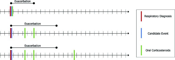
Our approach phenotypes an exacerbation when three components are observed in close temporal proximity: (i) a qualifying clinical encounter, (ii) a co-occurring respiratory diagnosis, and (iii) a prescription for, or administration of, oral corticosteroids. We define an exacerbation as beginning if a patient’s EHR includes one of several types of clinical encounters, co-occurring with a respiratory diagnosis code recorded on the same date, and followed within seven days by a prescription of oral corticosteroids. Any further prescriptions of oral corticosteroids within five days of the last prescription are considered extensions of the same exacerbation. The full interval of the exacerbation begins with the co-occurring encounter and respiratory diagnosis and ends five days after the last oral corticosteroid prescription. This approach is illustrated in Figure 1.

Figure 1:

An illustration of the exacerbation phenotyping task. The figure shows three example patient timelines and the resulting exacerbation event that is recognized in each. Short, vertical black lines on the timeline represent days. Vertical red, blue and green lines represent events recorded in the EHR. The duration of a phenotyped exacerbation is represented by the extent of the corresponding horizontal black line over the timeline.

A qualifying clinical encounter is detected by meeting one of the following conditions: (i) an encounter with type Hospital Encounter, Office Visit, Telephone, Orders Only, or of the generic type Appointment when additionally associated with a visit type of Office Visit, (ii) a recorded encounter associated with an inpatient or urgent care department, or (iii) a charge associated with a CPT code in the range 99221-99223 (initial hospital care), 9923199233 (subsequent hospital care), 99251-99255 (inpatient consultation), or 99281-99285 (emergency department visit). The associated respiratory diagnosis codes that can indicate the start of an exacerbation are ICD-9 493.x (asthma), 46[0-6].x (acute respiratory infections), 48[0-6].x (pneumonia), 490.x (bronchitis nos), 491.x (chronic bronchitis), 519.x (other diseases of respiratory system), or 786.x (symptoms involving respiratory system and other chest symptoms).

Predicting Asthma Exacerbations: Given our phenotyping algorithm to identify exacerbations in electronic health records, we can use supervised learning methods to train models that try to predict these exacerbations in advance. There are various ways in which this task can be framed. Here we approach the problem as a classification task: given a patient’s history up to a given decision date, we want our model to predict whether the patient will experience an exacerbation within the next 90 days or not. The event window of 90 days was selected because follow-up visits for asthma tend to be 3-6 months based on guideline recommendations. In this section, we describe three approaches we have used to learn classification models for this task.

We have investigated a number of variable representations for this task. One approach is to represent static and time-stamped event variables together using a fixed-length vector representation, comprising a summary of the event variables concatenated with the static variables. Alternatively, we can represent event variables by formulating a sequence of vectors for each patient, with each vector representing the events at a given time-stamp. This sequence, together with a fixed-length vector representing the static variables, forms a representation that preserves the patient’s temporal history instead of summarizing it.

The first learning method we apply is logistic regression with L ₁ and L ₂ regularization^11,12. Here we use a fixed-length vector representation comprising binary variables to represent the occurrence of each event variable in each of two different temporal windows: (i) over the last six months, and (ii) over the entire observation period, prior to the decision date. We perform internal cross-validation to tune the strength of the regularization.

A second learning method we apply to this task is a random forest¹³. We test two different fixed-length vector representations here: with event variables summarized based on (i) their occurrence in different temporal windows (as for logistic regression), and (ii) recency. In the latter case, for each event type (e.g. for each possible diagnosis), we include a numeric variable whose value represents the number of days since the last occurrence of the event. For example, a single variable in this representation indicates how long it has been since the patient has had an ICD-9 code in the 020.xx range. In the case in which a patient has not had the event recorded within the period covered by our data set, we set the variable value to ∞. Note that, for random forests, the scale of each variable is not important, and thus values of ∞ are not problematic since it is the relative ordering of variable values that matters. We tune the maximum tree depth as well as the number of sampled variables per split using internal cross-validation.

A third learning method we apply is a Long Short-Term Memory (LSTM) neural network¹⁴. In contrast to the logistic regression and the random forest, where the variables summarize the patient’s temporal history, the LSTM network is able to directly process the sequence of events in the history. However, some event types, namely problem diagnoses, other diagnoses, and interventions (procedures and medications), comprise large vocabularies (our cohort includes observations of 4,398 problem diagnoses, 6,533 other diagnoses, and 8,745 interventions) of which only a small subset is recorded at each encounter. Instead of working directly with the resulting sparse, high-dimensional vectors, we first map these event types to an embedded space, resulting in dense, lower-dimensional vectors that are then used to form the event sequence for the LSTM. To learn the weights for the embedding layer, we use Med2Vec¹⁵, a method that obtains distributed representations of medical concepts, while capturing the context represented by the ordering of EHR visits as well as the co-occurence of codes within an EHR visit. Separate embeddings of size 200 are generated for problem diagnoses, other diagnoses, and interventions. These are then concatenated, along with the other event variables, to produce the event representation at each time-stamp in the record. The ordered sequence of events forms the input sequence for the LSTM. We use an LSTM cell state of size 100 and a sigmoid output layer. The static demographic variables feed directly into the output layer. For the loss function, we use binary cross-entropy with L ₂ regularization. Figure 2 shows the LSTM network architecture.

Figure 2:

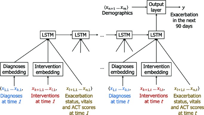
The LSTM network for predicting exacerbations. Time-stamped event variables x ₁ … x _n are represented by formulating a sequence of vectors, with each vector representing the events at a given time-stamp x _1,t ... x _n,t. Diagnoses and interventions are embedded into dense, lower-dimensional vectors. The static demographic variables x _n+1 … x _m feed directly into the output layer of the network.

Identifying Subpopulations of Asthma Patients: To address the second task of identifying subpopulations of patients who share common temporal/seasonal patterns in their exacerbations, we develop a clustering approach based on a mixture of semi-Markov models. The motivation for this approach is to identify groups of patients who have commonality in the (i) durations of their exacerbations, (ii) durations of periods in which their asthma is controlled, and (iii) seasonal dependence of their exacerbations.

As illustrated in Figure 3a, the data that is input to this approach consists of a state sequence for each patient along with a duration for each state. We can think of each patient as transitioning between two states, exacerbated and controlled, or perhaps remaining in the controlled state throughout the observation period. Since we cannot detect an exacerbation that starts before our observation period, we assume that all patients are in the controlled state at the beginning of their sequence. Moreover, because these sequences are both left- and right-censored (i.e., we observe the state sequence only for the period from January 1, 2007 to December 31, 2011), we divide the general controlled state into three separate states: first-controlled, internal-controlled, and last-controlled. Since we assume that all patients are in a controlled state at the beginning of a sequence, all sequences begin with a first-controlled state. An internal-controlled state represents the period between two exacerbated states during which a patient’s asthma is controlled. Only patients who are recorded as having at least two exacerbated states during the study period have internal-controlled states. Finally, patients who have had at least one exacerbated state will also have a last-controlled state. With this partitioning of the controlled states, we can separately estimate the durations of sojourns in the internal-controlled state thereby avoiding the bias that would be imposed in estimating controlled state durations by also including the censored durations of the first-controlled and last-controlled states.

Figure 3:

Modeling exacerbation state sequences using a semi-Markov model. (a) Example state sequences for three patients. (b) A semi-Markov model for characterizing asthma exacerbations. Nodes represent states and edges represent allowable transitions. Aside from the silent start and end states, each state has a duration distribution.

Each state has an associated duration (with days as the units), and thus we can represent patient p’s exacerbation history as follows:

$${\text{S}}^{(p)}\equiv \langle s_1^{(p)},\cdot \cdot \cdot ,s_{L_p}^{(p)}\rangle ,{\text{d}}^{(p)}\equiv \langle d_1^{(p)},\cdot \cdot \cdot ,d_{L_p}^{(p)}\rangle$$

Where s^(p) represents the state sequence for patient p, d^(p) represents the corresponding duration sequence, $s_i^{(p)}$ represents the ith state in patient p’s history, $d_i^{(p)}$ represents the duration of this ith state, and L _p represents the length of the history in terms of the number of state visits. A semi-Markov model¹⁶ represents the probability of a patient’s history as:

$$P({\text{S}}^{(p)},{\text{d}}^{(p)})=P(s_1^{(p)}|\text{start)\hspace{0.17em}}P(d_1^{(p)}|s_1^{(p)}){\displaystyle \prod _{i=2}^{L_p}[P(s_i^{(p)}|s_{i-1}^{(p)})P}(d_i^{(p)}|s_i^{(p)})]P(\text{end\hspace{0.17em}}|s_i^{(p)})$$

where each $P(s_i^{(p)}|s_{i-1}^{(p)})$ term represents astate-transition probability, and each $P(d_i^{(p)}|s_i^{(p)})$ term represents the probability of staying in state $s_i^{(p)}$ for the duration $d_i^{(p)}$. Because we assume that all sequences begin in the first-controlled state, P (first-controlled | start) = 1. Likewise, P (end | last-controlled) = 1. Figure 3b depicts the states and transitions for such a model.

In order to capture the effect of seasonal determinants of exacerbations, we can extend the above model to use in-homogenous duration distributions for the controlled states. Specifically, our approach uses distinct duration distributions for the controlled states conditioned on the month in which the patient entered the controlled state. In this way, the timing of a patient’s transition to the exacerbated state can depend on the time of year. To implement this inhomogeneity, we extend the represention of patient p’s exacerbation history to indicate the month $m_i^{(p)}$ in which each state $s_i^{(p)}$ is entered:

$${\text{s}}^{(p)}\equiv \langle s_1^{(p)},\mathrm{...},s_{L_p}^{(p)}\rangle ,{\text{d}}^{(p)}\equiv \langle d_1^{(p)},\mathrm{...},d_{L_p}^{(p)}\rangle ,{\text{m}}^{(p)}\equiv \langle m_1^{(p)},\mathrm{...},m_{L_p}^{(p)}\rangle$$

We then condition on the month sequence when determining the probability of the states and durations:

$$P({\text{s}}^{(p)},{\text{d}}^{(p)}|m^{(p)})=P(s_1^{(p)}|\text{start)\hspace{0.17em}}P(d_1^{(p)}|s_1^{(p)}){\displaystyle \prod _{i=2}^{L_p}[P(s_i^{(p)}|s_{i-1}^{(p)})P}(d_i^{(p)}|s_i^{(p)},m_i^{(p)})]P(\text{end\hspace{0.17em}}|s_{L_p}^{(p)}).$$

Note that, in this formulation, the duration of the sojourn in the first state does not depend on the month since all of our sequences begin on the same date. Additionally, for $P(d_i^{(p)}|last-controlled,m_i^{(p)})$ and $P(d_i^{(p)}|exacerbated,m_i^{(p)})$ in our models, there is no dependence on $m_i^{(p)}$. We make this choice for the last-controlled state because our durations in this state are censored and hence not informative. Although it would be reasonable to have the duration distribution for the exacerbated state depend on the month, we posit that there is not a strong dependence here and choose not to incorporate it into our representation.

To represent duration distributions, we use histograms at the time granularity of days. The duration for all states is capped at 1,826 days (five years) which is the length of our patient histories. All controlled states have a minimum duration of one day and the exacerbated state has a minimum duration of five days (since our exacerbation phenotyping procedure specifies this as the minimum duration). To contend with the sparsity of our data when estimating durations, we use Gaussian kernel density estimation (with bandwidth = 0.3) followed by discretization to days to smooth the histograms.

In order to cluster patients into distinct subpopulations, we construct a mixure of semi-Markov models as shown in Figure 4. Each component of the mixture incorporates the set of states shown in Figure 3b, aside from there being a common start state. Thus, for example, instead of having one first-controlled state, there is one per component. The transition probabilities from the start state represent prior probabilities of mixture components (i.e., mixture weights). By allowing the parameters in the component semi-Markov models to vary from one component to another, we can learn state transitions and duration distributions that characterize different subpopulations.

Figure 4:

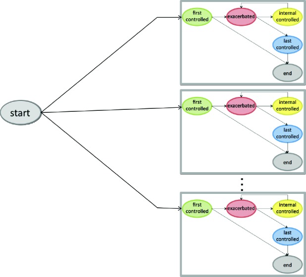
A mixture of semi-Markov models for characterizing asthma exacerbations. The mixture components are shown enclosed in gray boxes.

We learn the parameters for our mixture of semi-Markov models using an Expectation Maximization approach. To initialize the duration parameters for each state, we randomly select from the training set 10 events corresponding to the given state (and month when applicable) and use these events to estimate the associated duration distribution. The transitions going out of each state are initialized to a uniform distribution. To mitigate the effect of local optima in the EM procedure, the parameter estimation process is restarted 10 times, each time re-initializing the model with a different randomly selected subset of events from the training data. For a given number of components k, we then select the model that maximizes the likelihood of the training-set data.

Results

In this section, we describe our results from phenotyping asthma exacerbations from EHRs, predicting near-term exacerbations, and identifying subpopulations of asthma patients who have similar exacerbation patterns.

Phenotyping Asthma Exacerbations: We applied our asthma exacerbation phenotyping algorithm to the electronic health records for 28,101 asthma patients. The algorithm identified a total of 14,447 exacerbations in these records. Figure 5 shows how the frequency of exacerbations varies by time of year in our patient cohort. Several notable features are present in this plot, including a spring peak corresponding to pollen-triggered exacerbations, an early fall peak corresponding to the increase in respiratory virus illness as children return to school, and a smaller peak centered on the holiday travel season.

Figure 5:

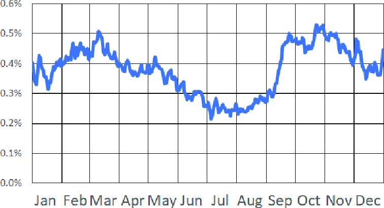
Plot of exacerbation frequency by time of year in our cohort. The y-axis represents the percentage of patients in our cohort who are in the midst of an exacerbation event on a given day of the year.

Predicting Asthma Exacerbations We evaluate our supervised learning approach for predicting asthma exacerbations using 10-fold cross-validation. In the present study, we consider one decision date per patient. For a patient in the training set, we train on data in the patient’s EHR that precedes the decision date and determine the class label for the patient according to whether they experienced an exacerbation within 90 days after the decision date or not. For a patient in the test set, a learned model is given data in the patient’s EHR that precedes the decision date, and then predicts whether the patient will have an exacerbation within the next 90 days.

To ensure that our models are seasonally independent, we choose decision dates such that they are uniformly distributed throughout the days of the year, and we have at least 90 days on record after the decision date for each patient. Moreover, we left-censor the patient histories as needed to ensure that we have observation periods of the same length for every patient.

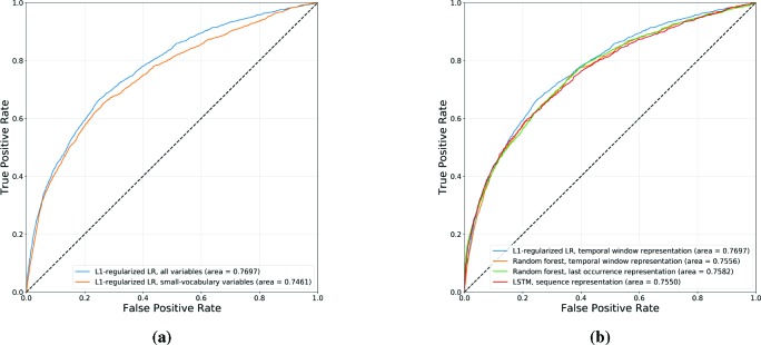
Figure 6a shows the receiver operating characteristic (ROC) curves for logistic regression models learned using L1 regularization over a fixed-length representation based on the occurrence of event variables in two temporal windows: (i) spanning the last six months, and (ii) spanning the entire observation period prior to the decision date. We show results with and without the inclusion of the large-vocabulary variables in the EHR, namely the problem diagnoses, other diagnoses and interventions (medications and procedures). In this way, we can evaluate the predictive value gained from the inclusion of these richer but more complex EHR variables for the purpose of predicting asthma exacerbations. L2-regularized logistic regression models were also learned and evaluated, but yielded lower area under the curve (AUC) values than the L1-regularized models.

Figure 6:

ROC curves for asthma exacerbation prediction, comparing (a) L₁-regularized logistic regression models, with and without the inclusion of large-vocabulary EHR categories (diagnoses and interventions), and (b) the best-performing logistic regression model (L₁ regularization and a temporal window-based representation), random forests (temporal window-based and last occurrence-based representations), and LSTM (sequence-based representation).

The results shown in Figure 6a suggest that, given an asthma patient’s past electronic health record, we are able to predict whether they will have an exacerbation in the near future with some degree of accuracy. The inclusion of large-vocabulary variables yields a small but significant boost in AUC, indicating the value of these richer but more complex variables in predicting exacerbations.

Figure 6b shows ROC curves comparing multiple classifiers and representations used to predict asthma exacerbations, namely: (i) the best-performing logistic regression model, using L₁ regularization and a temporal window-based representation, (ii) random forest models using temporal-window and last occurrence-based representations, and (iii) the LSTM model using a sequence-based representation. Notably, logistic regression outperforms the more complex models given the same representation (random forest) as well as richer representations (random forest, LSTM).

In order to gain insight into which EHR variables are most valuable in predicting asthma exacerbations, we analyze the best-performing L1 logistic regression model by ranking its coefficients in decreasing order of magnitude, and list the top-25 associated variables in Table 1. These results suggest that while exacerbations in the last six months are the single greatest predictor for exacerbations in the near future, a diverse set of variables are useful as predictors. Perhaps surprisingly, the majority of the most important variables correspond to events observed at any point in the patient’s past observation period, as opposed to more recent events observed in the last six months. While small-vocabulary variables such as previous exacerbations, ACT scores, vitals and demographics provide significant predictive value (as indicated in Figure 6a), the large-vocabulary variables (diagnoses and interventions) dominate the list of most important predictors upon their inclusion. Notably, some asthma diagnosis codes are negatively associated with future exacerbations. A possible explanation is that these codes tend to be associated with less acute cases of asthma.

Table 1:

Top-25 variables of L1-regularized logistic regression model by coefficient magnitude.

Coef	Window	Category	Variable
0.90	6 Months	Exacerbations	Asthma exacerbation
0.48	Ever	Prescription meds	Corticosteroids
0.41	Ever	Diagnoses	V58.65: Long-term (current) use of steroids
0.35	Ever	Exacerbations	Asthma exacerbation
0.29	Ever	Procedures	Periodic preventive medication, infant
-0.27	Ever	Problem diagnoses	493.90: Unspecified asthma
-0.22	Ever	Diagnoses	493.81: Exercise induced bronchospasm
-0.22	Ever	Problem diagnoses	493.00: Extrinsic asthma, unspecified
0.21	Ever	Procedures	Hospital discharge day management < 30 min
-0.21	Ever	Diagnoses	493.90: Unspecified asthma
-0.18	N/A	Demographics	Race: White
0.18	Ever	Administered meds	Anticholinergics
-0.17	Ever	Procedures	Office outpatient visit < 5 min
0.17	6 Months	Procedures	Office outpatient visit < 15 min
0.17	Ever	Procedures	Breathing capacity test
-0.16	Ever	Diagnoses	V03.89: Other specified vaccination
0.15	6 Months	Charges	IV infusion therapy/prophylaxis
0.15	6 Months	Diagnoses	493.90: Unspecified asthma
-0.14	Ever	Procedures	Urinalysis
0.13	Ever	Prescription meds	Penicillin Combinations
-0.13	Ever	Procedures	Office outpatient visit < 15 min
0.12	Ever	Procedures	Residual lung capacity
0.12	Ever	Diagnoses	493.92: Unspecified asthma with acute exbn
0.12	Ever	Charges	HB-visit units 46+ minutes room usage
0.12	N/A	Demographics	Age: 55-60 Years

Identifying Subpopulations of Asthma Patients For the second task considered, we evaluate our mixture of semi-Markov model approach to clustering patients by partitioning our patients such that 80% of them are in a training set, and the remaining 20% are in a test set. For each specified number of mixture components, k, we learn a model using data from patients in the training set. We then evaluate the model by determining the likelihood of the test-set patients under that model. To mitigate the effect of local optima in the EM procedure, we use 10 multiple random restarts for a given value of k and then select the model that maximizes the likelihood of the training-set data.

Figure 7 shows the resulting test-set log likelihoods for values of k ranging from 1 (a single semi-Markov model) to 35. We can draw several conclusions from these results. First, the models with multiple components explain the test-set data better than the individual semi-Markov model. Second, the log likelihood keeps rising as we add components to model until about 20, and it then levels off. Even with 35 components, however, we do not see evidence of overfitting.

Figure 7:

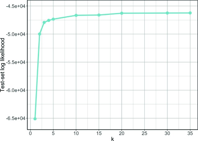
Log likelihood of the test set data as the number of components, k, is varied.

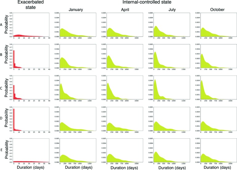
To gain insight from the models, we can inspect the learned parameters. Figure 8 shows selected duration distributions from a learned mixture of semi-Markov models when the number of components k = 5. Each row represents a component. The first column shows the duration distribution for the exacerbated state, and subsequent columns show duration distributions for the internal-controlled state conditioned on entering the state in the months of January, April, July or October. Recall that the internal-controlled state has a separate duration distribution for each month of the year; we show the distributions for only four months due to space limitations. Table 2 shows the transition probabilites for each component in the mixture.

Figure 8:

Selected duration distributions from the mixture of semi-Markov models. Each row shows a selection of the learned state duration distributions for a mixture component in a 5-component model. The first column shows the duration distribution for the exacerbated state. Subsequent columns show duration distributions for the internal-controlled state, conditioned on entering the state in January, April, July or October.

Table 2:

Transition probabilities for the 5-component mixture of semi-Markov models.

Component	Transition probabilities
	first-controlled to	exacerbated to
	exacerbated	internal-controlled
A	0.7509	0.7317
B	0.9965	0.2150
C	0.9981	0.5894
D	0.9985	0.5237
E	0.0003	0.4996

The distributions shown in Figure 8 and Table 2 illustrate several notable differences among the components. Component A mostly represents patients who struggle to keep their asthma under control. Within this component, the duration distribution for the exacerbated state has a long tail, and the probability of transitioning to the internal-controlled state is relatively high indicating that many patients in this component have experienced multiple exacerbations during the observation period. However, this component also seems to represent the patients who did not experience any exacerbations during the observation period. This is indicated by the relatively low transition probability (0.7509) from the first-controlled state to the exacerbation state. The patients who do not take this transition remain in the first-controlled state for the entirety of the observation period. Component B represents patients who have infrequent exacerbations. This is indicated by the relatively low probabability of transitioning from the exacerbated state to internal-controlled state, meaning that most of these patients had only one exacerbation during the observation period. Components C and D are similar to one another

except that patients in the former generally have somewhat more prolonged exacerbations and shorter sojourns in the internal-controlled state. Component E represents patients who rarely, if ever, experience exacerbations. The probability of transitioning to the exacerbated state is near zero and the duration distributions are very close to their initialized values.

The internal-controlled duration distributions show heterogeneity across the months, generally being more peaked in the proximity of fall. However, with the 5-component model, we do not see components with pronounced specificity for seasonal exacerbation patterns (e.g., we do not see a component that obviously corresponds to fall exacerbators). We see such clusters in some of the models with more components.

These results demonstrate that our mixture of semi-Markov models approach is able to identify subpopula-tions of patients who exhibit meaningful differences in the temporal patterns of their exacerbations.

Discussion

We have presented approaches and empirical results that address two key tasks in modeling asthma exacerbations from electronic health records. First, we considered to what extent exacerbations can be predicted given a pa-tient’s clinical history as represented in their electronic health record. Our results indicate that learned models are able to predict exacerbations with a moderately high degree of accuracy (AUC ≈ 0.77) when given such information. The ability to predict asthma exacerbations is important to identify the patients that require more aggressive treatment plans and closer medical followup to improve patient outcomes. Second, we considered whether distinct temporal exacerbation phenotypes can be elicited from EHR data. Our approach to this task, which is based on a mixture of semi-Markov models, was able to identify subpopulations of asthma patients sharing distinct temporal and seasonal patterns in their exacerbation susceptibility.

There are several directions of future work that we plan to explore. First, we plan to investigate whether the mixture of semi-Markov models approach can lend value to our supervised learning approaches for predicting exacerbations. One way in which we might do this is by using the mixture model to cluster each patient based on their past exacerbation history and then computing a seasonally varying, cluster-specific risk score that is another input variable for the exacerbation-prediction models. Second, we plan to extend our exacerbation-prediction models by incorporating environmental variables. We also plan to investigate other formulations of the exacerbation-prediction problem, such as addressing it as a time-to-event task.

References

- 1.To T., et al. Global asthma prevalence in adults: Findings from the cross-sectional world health survey. BMC Public Health. 2012;12(204):1471–2458. doi: 10.1186/1471-2458-12-204. [DOI] [PMC free article] [PubMed] [Google Scholar]
- 2.Winer R. A., et al. Asthma incidence among children and adults: findings from the BRFS system asthma call-back survey–United States, 2006-2008. Journal ofAsthma. 2012;49(1):16–22. doi: 10.3109/02770903.2011.637594. [DOI] [PubMed] [Google Scholar]
- 3.Dougherty R. H., Fahy J. V. Acute exacerbations of asthma: Epidemiology, biology and the exacerbation-prone phenotype. Clinical and Experimental Allergy. 2009;39(2):193–202. doi: 10.1111/j.1365-2222.2008.03157.x. [DOI] [PMC free article] [PubMed] [Google Scholar]
- 4.Wark P. A. B., Gibson P. G. Asthma exacerbations 3: Pathogenesis. Thorax. 2006;61(10):909–915. doi: 10.1136/thx.2005.045187. [DOI] [PMC free article] [PubMed] [Google Scholar]
- 5.Bateman E., et al. Development and validation of a novel risk score for asthma exacerbations: The risk score for exacerbations. Journal of Allergy and Clinical Immunology. 2015;135(6):1457–1464. doi: 10.1016/j.jaci.2014.08.015. [DOI] [PubMed] [Google Scholar]
- 6.Hoch H., et al. Can we predict fall asthma exacerbations? Validation of the seasonal asthma exacerbation index. Journal of Allergy and Clinical Immunology. 2017;140(4):1130–1137. doi: 10.1016/j.jaci.2017.01.026. [DOI] [PMC free article] [PubMed] [Google Scholar]
- 7.Loymans R., et al. Exacerbations in adults with asthma: A systematic review and external validation of prediction models. Journal of Allergy and Clinical Immunology. 2017;140(4):1130–1137. doi: 10.1016/j.jaip.2018.02.004. [DOI] [PubMed] [Google Scholar]
- 8.Reddel H., et al. An official ATS/ERS statement: Asthma control and exacerbations: Standardizing endpoints for clinical asthma trials and clinical practice. American J. Respiratory Critical Care Medicine. 2009;180(1):59–99. doi: 10.1164/rccm.200801-060ST. [DOI] [PubMed] [Google Scholar]
- 9.Busse W., Morgan W., Taggart V., Togias A. Asthma outcomes workshop: Overview. Journal ofAllergy and Clinical Immunology. 2012;129(3 Suppl):S1–S8. doi: 10.1016/j.jaci.2011.12.985. [DOI] [PMC free article] [PubMed] [Google Scholar]
- 10.Global Initiative for Asthma. Global strategy for asthma management and prevention. 2019 www.ginasthma.org. [Google Scholar]
- 11.Hoerl, Kennard R. Ridge regression: Biased estimation for nonorthogonal problems. Technometrics. 1970;12(1):55–77. [Google Scholar]
- 12.Tibshirani R. Regression shrinkage and selection via the lasso. Journal of the Royal Statistical Society, Series B. 1996;58(1):267–288. [Google Scholar]
- 13.Breiman L. Random forests. Machine Learning. 2001;45(1):5–32. [Google Scholar]
- 14.Hochreiter S., Schmidhuber J. Long short-term memory. Neural Computation. 1997;9(8):1735–1780. doi: 10.1162/neco.1997.9.8.1735. [DOI] [PubMed] [Google Scholar]
- 15.Choi E., et al. Multi-layer representation learning for medical concepts; Proceedings of the 22nd ACM SIGKDD International Conference on Knowledge Discovery and Data Mining; ACM; 2016. pp. 1495–1504. [Google Scholar]
- 16.Rabiner L. R. A tutorial on hidden Markov models and selected applications in speech recognition; Proceedings of the IEEE; 1989. pp. 257–286. [Google Scholar]