Habitat productivity is a poor predictor of body size in rodents

Abstract

The “resource availability hypothesis” predicts occurrence of larger rodents in more productive habitats. This prediction was tested in a dataset of 1,301 rodent species. We used adult body mass as a measure of body size and normalized difference vegetation index (NDVI) as a measure of habitat productivity. We utilized a cross-species approach to investigate the association between these variables. This was done at both the order level (Rodentia) and at narrower taxonomic scales. We applied phylogenetic generalized least squares (PGLS) to correct for phylogenetic relationships. The relationship between body mas and NDVI was also investigated across rodent assemblages. We controlled for spatial autocorrelation using generalized least squares (GLS) analysis. The cross-species approach found extremely low support for the resource availability hypothesis. This was reflected by a weak positive association between body mass and NDVI at the order level. We find a positive association in only a minority of rodent subtaxa. The best fit GLS model detected no significant association between body mass and NDVI across assemblages. Thus, our results do not support the view that resource availability plays a major role in explaining geographic variation in rodent body size.

Rodent species are 1) largely variable in body size (Nowak 1999; Jones et al. 2009; Alhajeri and Steppan 2016), 2) have a wide geographic range (Fabre et al. 2012), and 3) constitute most mammal species (Wilson and Reeder 2005). These characteristics make rodents suitable for making inferences about mammals and especially amenable to macroecological studies (e.g., Cano et al. 2014; Amori et al. 2015; Alhajeri 2016, 2018; Maestri et al. 2016, 2017; Alhajeri and Steppan 2018a, 2018b). Such studies investigate the relationship between species’ traits and geographic/environmental variables across their range (Brown 1995; Blackburn and Gaston 2003; Smith and Lyons 2011), often at large spatial scales (Brown and Maurer 1989; Beck et al. 2012). Macroecology can examine patterns within a single species, across species, and across assemblages (Meiri 2011); patterns may also be examined at different geographic scales (i.e., single continent vs. worldwide) (Beck et al. 2012). Observations made at narrow geographic and taxonomic scales do not always scale up (Berke et al. 2013), and patterns observed in geographic region do not always apply to others (Meiri et al. 2004; Rodríguez et al. 2008; Berke et al. 2013). This may reflect regional environmental differences (Rodríguez et al. 2008).

Bergmann’s (1847) rule documents a pattern of increased body size in high latitudes (cold environments) and is among the oldest and most studied macroecological patterns (Gaston and Blackburn 2000; Meiri and Dayan 2003; Blackburn and Hawkins 2004; Maestri et al. 2016; Shelomi and Zeuss 2017; Riemer et al. 2018). This rule is generally observed in endothermic animals (Freckleton et al. 2003; Meiri and Dayan 2003; Rodríguez et al. 2008; Carotenuto et al. 2015). The heat conservation hypothesis is a common explanation for Bergmann’s rule, where increased body size conserves heat via decreased surface-area-to-volume ratio (Bergmann 1847; Mayr 1956; Blackburn and Hawkins 2004). So far, support for Bergmann’s rule is weak or absent in rodents in general (e.g., Meiri and Dayan 2003; Alhajeri and Steppan 2016; Gohli and Voje 2016; Maestri et al. 2016; Mori et al. 2019).

The resource availability hypothesis predicts a positive association between body size and the amount of food resources in a habitat (Rosenzweig 1968; Blackburn et al. 1999; Blackburn and Hawkins 2004; Virgós et al. 2011). More productive habitats have greater resources and as such may be associated with larger body size (Blackburn and Hawkins 2004; McNab 2010). In many terrestrial habitats, primary productivity is inversely related to latitude (Leith and Whittaker 1975; Gillman et al. 2015). Thus, the resource availability hypothesis may lead to a pattern that is opposite to Bergmann’s rule—an increase in body size in low latitudes. Previous rodent studies found some association between body size and indirect habitat productivity measures (e.g., precipitation, latitude, and altitude) (e.g., Taylor et al. 1985; Medina et al. 2007; Alhajeri and Steppan 2016; Maestri et al. 2016; García-Mendoza et al. 2018). Direct measures of habitat productivity (such as vegetation biomass) have been seldom used, possibly due to the difficulty of their estimation in the past.

Here, we investigate the association between rodent body size and habitat productivity using a direct habitat productivity measure, the normalized difference vegetation index (NDVI) (see Bannari et al. 1995), which is good proxy for vegetation biomass in many ecosystems (e.g., Gamon et al. 2013; Yu et al. 2013; Gao et al. 2016; Zhu et al. 2017). We study this association at a large spatial and taxonomic scale—both across species and across assemblages. We study this association based on a large sample size that includes both large- and small-sized rodent species. Based on the resource availability hypothesis, we predict that differences in NDVI values explain geographic variation in rodent body mass. More specifically, we expect a positive relationship between these variables. Because temperature and productivity are often statistically independent (Rosenzweig 1968; Virgós et al. 2011), we may find support for the resource availability hypothesis in rodents despite not finding support for Bergmann’s rule in this group (Alhajeri and Steppan 2016).

Materials and Methods

Data extraction

We used the same 1,315 rodent species dataset from Alhajeri and Steppan (2016) and Alhajeri and Fourcade (2019). This dataset includes mean species body mass (a proxy for body size) from PanTHERIA (Jones et al. 2009); along with the annual mean temperature (BIO1; in °C) and the annual precipitation (BIO12; in millimeters) of each species’ habitat (Supplementary Table S1). The climatic variables (BIO1 and BIO12) were extracted at a spatial resolution of 2.5 arc min from WorldClim (Hijmans et al. 2005), covering the 1950–2000 time period. Alhajeri and Steppan’s (2016) method of extracting species-level bioclimatic data involved cross-referencing WorldClim global climate layers with geographic range data for each species obtained from the International Union for Conservation of Nature Red List (IUCN 2015), and then obtaining the mean value of each bioclimatic variable across the geographic range of each species. The same method was used to estimate habitat productivity using IUCN geographic range data (see below).

We estimated the productivity of each rodent species’ habitat using a commonly used vegetation index, the NDVI (see Bannari et al. 1995). This index is a quantitative measure of vegetation biomass, cover, health, and productivity in various terrestrial ecosystems (e.g., Gamon et al. 2013; Yu et al. 2013; Gao et al. 2016; Zhu et al. 2017). Chidodo (2017) recently detected a positive correlation between rodent abundance and NDVI. This indicates that NDVI can capture aspects of habitat productivity that are relevant for rodents. NDVI is based on visible and near-infrared light reflected by vegetation and is correlated with photosynthetic activity, and thus serves as a quantitative measure of how “green” a habitat is (Myneni et al. 1995). NDVI is unitless, and ranges from −1 to +1, where values close to zero (including negative values) indicate barren regions (bare soil, rock, sand, snow, and water), moderate values indicate sparsely vegetated areas such as grasslands, and high values indicate densely vegetated areas (i.e., highly productive regions) such as forests (Bhandari et al. 2012; Saravanan et al. 2019).

We use Pinzon and Tucker’s (2014) third generation NDVI dataset (NDVI_3g), obtained from the National Oceanic and Atmospheric Administration’s (NOAA) Advanced Very High-Resolution Radiometer (AVHRR) sensors, from the Global Inventory Modelling and Mapping Studies (GIMMS), provided by the National Aeronautics and Space Administration (NASA, https://nex.nasa.gov/nex/projects/1349/). We used the GIMMS library (Detsch 2018) in R (R Development Core Team 2018) to download the global AVHRR GIMMS NDVI_3g dataset—we used the latest version of the dataset (NDVI_3g.v1), which is updated from the NDVI_3g.v0 (Pinzon and Tucker 2014), and provides NDVI values for the period of July 1981 to December 2015, twice a month (half-monthly), with a spatial resolution of one-twelfth degree (∼8 km). We also used the GIMMS library to: 1) rasterize the NDVI_3g data, 2) perform quality control, by discarding all nonreliable NDVI_3g values, or “flagged” pixels that have either been spline-interpolated (flag value = 1) or possibly represent snow or cloud cover (flag value = 2), and 3) aggregate half-monthly NDVI_3g datasets into monthly maximum-value composites (MVC). The MVC procedure is a common preprocessing step in satellite imaging, and allows for the reduction of measurement error rates, such as those caused by variation in the atmosphere and sensor angle (Holben 1986). In the case of NDVI data, MVC involves a pixel-by-pixel comparison of half-monthly data for each month, and the retention of only the highest NDVI value for each pixel location (Holben 1986). This resulted in a total of 414 MVC NDVI values for each pixel location (spanning each month from July 1981 to December 2015).

Cross-species analysis

We used the R library RASTER (Hijmans 2018) to extract the 414 MVC NDVI values of all pixels that fall within each species’ geographic range. These geographic ranges were based on IUCN polygon shape files (previously extracted in Alhajeri and Steppan 2016), which were read into R using the RGDAL library (Bivand et al. 2018). We then calculated both the mean and the median of these MVC NDVI values for each species (Supplementary Table S1). Based on Kendall’s tau (τ) coefficient (Kendall 1938), these mean and the median MVC NDVI values were highly (positively) correlated (P < 0.0001, τ = 0.953), indicating that they may provide similar information. Consequently, only the mean MVC NDVI values were used in subsequent analyses (referred to as “species-level NDVI” values in the rest of the article). We used these values as estimates of the typical productivity of the habitat occupied by each species.

We examined the association between species-level NDVI values and each of the corresponding 1) annual mean temperature (BIO1) and 2) annual precipitation (BIO12) values, using Kendall’s τ (see above). As a nonparametric test, Kendall’s τ does not assume normality, and is less sensitive to outliers than parametric correlation coefficients, such as Pearson’s r (Daniel 1990).

The association between species-level NDVI values and mean species body mass was examined using phylogenetic generalized least squares (PGLS) analysis (Harvey and Pagel 1991), as implemented in the R library CAPER (Orme et al. 2018). This method accounts for the phylogenetic relatedness of examined taxa (Harvey and Pagel 1991; Orme et al. 2018). The phylogenetic covariance matrix used in the PGLS analysis was estimated by weighting the covariances by Pagel’s lambda (λ), which was estimated from model residuals. A value of λ = 1 denotes a Brownian motion model, λ = 0 indicates the absence of phylogenetic signal, and 0<λ < 1 denotes and intermediate model (Pagel 1999).

PGLS analyses were carried out using Fabre et al.’s (2012) supermatrix chronogram. Since the PGLS analysis requires a fully bifurcating tree, polytomies were randomly resolved, while being assigned an internal branch length of zero, following Alhajeri and Steppan (2016). Out of all the examined data transformations, the combination that fit the assumptions of the PGLS model best (i.e., residuals’ normality and homogeneity), was a natural log transformation of mean species body mass (“species-level body mass”) and raw (untransformed) species-level NDVI values—this setup was used in all PGLS analyses.

Uncertainty in the estimates of species-level body mass is a potential source of error in interspecific data, especially across broad phylogenetic scales that encompass >1,000 species. To investigate if error in species-level body mass estimates could affect the overall results, we employed Maestri et al.’s (2017) sampling approach (see below). PanTHERIA provides point estimates for average body mass for each species, without uncertainty values, as such, we randomized species-level body mass (µ) values 1,000 times for each species, around a 30% confidence interval (an arbitrary, but conservative value), which defines the lower (µ −30%) and the upper (µ +30%) intervals for the randomizations, calculated for each species-level body mass value (for details, see Maestri et al. 2017). A PGLS analysis was performed for each of the 1,000 vectors of randomized average values (Supplementary Table S2). The results from all 1,000 runs were summarized numerically and graphically.

Fourteen out of the 1,315 rodent species in the dataset of Alhajeri and Steppan (2016) were dropped from this study. These include 8 species for which species-level NDVI values could not be calculated (mostly due to having an extremely large range size) and 5 Neusticomys species that were included in Fabre et al.’s (2012) tree based on misidentified GenBank sequences. The order-level PGLS analysis was conducted on the remaining 1,301 rodent species that appear in Supplementary Table S1. A scatterplot was generated in the R base library to visualize the association between species-level NDVI values and species-level body mass values.

In addition to the order-level PGLS analysis, we also ran PGLS analyses at narrower taxonomic scales, including suborders, superfamilies, families, subfamilies, and genera. For each taxonomic level, only taxa with 10 or more species sampled in the group were analyzed. This was done to reduce common problems associated with small sample sizes, such as low statistical power and inflated Type I error rate (Forstmeier et al. 2017). This taxonomically partitioned analysis relied on taxonomic information from the Integrated Taxonomic Information System (ITIS 2018), which was retrieved using the R library TAXIZE (Chamberlain et al. 2018). The full data matrix used to carry out all cross-species analyses appears in Supplementary Table S1. This matrix also includes the ITIS taxonomic information for each species.

Cross-assemblage analysis

The association between body mass and NDVI values was also examined across rodent assemblages. In this approach, the species’ geographic ranges (IUCN polygons) were converted into a presence–absence matrix at a 1.5-degree grid resolution using the R library LETSR (Vilela and Villalobos 2015). We considered a species to be present in a given grid cell if its distribution covers any part of it (i.e., >0% of the grid cell). As such, each of the 1,301 rodent species used in the cross-species analysis (Supplementary Table S1) were found in at least one of the resulting grid cells. We removed all cells in the resulting grid where none of the examined species is present, resulting in a total of 7,721 cells (i.e., assemblages) with at least 1 of the 1,301 species present (Supplementary Table S3).

To calculate the mean NDVI value for each grid cell, we first used RASTER to project the raster of MVC NDVI values (see “Data extraction” section) to a new raster that matches the coordinate reference system and resolution of the presence–absence matrix. The NDVI values for this new raster were computed using bilinear interpolation, which is often used for continuous variables (Hijmans 2018). The “assemblage-level NDVI” values were calculated by taking the average of the 414 MVC NDVI values for each grid cell (Supplementary Table S4). NDVI values were missing in 199 out of the 7,721 grid cells. As such, the cross-assemblage analyses were conducted on the remaining 7,602 grid cells. The R libraries RGDAL and MAPTOOLS (Bivand and Lewin-Koh 2017) were used to map of the spatial distribution of assemblage-level NDVI values.

LETSR was used to assign a body mass value to each grid cell based on the presence–absence matrix. This “assemblage-level body mass” value for each grid cell was based on the average of the species-level body mass values of all species present inside the grid cell (Supplementary Table S4). As for NDVI, the R libraries RGDAL and MAPTOOLS were used to map of the spatial distribution of assemblage-level body mass values. In addition, a scatterplot was generated in the R base library to visualize the association between assemblage-level body mass values and assemblage-level NDVI values.

The association between assemblage-level body mass values and assemblage-level NDVI values across the 7,602 grid cells was determined using both ordinary least squares (OLS) and generalized least squares (GLS) regression analyses (Aitken 1934). R base library was used to conduct the OLS regression whereas GLS was conducted using the R library NLME (Pinheiro et al. 2017). GLS models were fit by maximizing the restricted log-likelihood function. We expect some degree of spatial autocorrelation in our dataset, whereby nearby grid cells have similar body mass and NDVI values (see Dormann et al. 2007). As such, we used NLME to fit 5 additional GLS models, each with a unique autocorrelation structure: 1) exponential, 2) Gaussian, 3) linear, 4) rational quadratics, and 5) spherical—for more details, see Pinheiro et al. 2017. In all 5 models, a nugget effect was assumed, and the spatial covariates were based on the distance between the longitude/latitude coordinates of the geographic centroids of the of the grid cells. By default, NLME measures the distance between the observations using Euclidean distance. In addition to Euclidean distance, we also constructed models that use the great-circle distance based on the haversine formula (Inman 1835). This formula considers Earth’s curvature and is thus useful at large spatial scales. We used Akaike information criterion (AIC) weights (wi) to assess model fit (Akaike 1974; Bozdogan 1987; Burnham and Anderson 2002; Wagenmakers and Farrell 2004)—calculated using the R library QPCR (Pabinger et al. 2014).

Results

Cross-species analysis

Species-level NDVI values were correlated with both annual mean temperature (BIO1) (P < 0.0001, τ = 0.348) and annual precipitation (BIO12) (P < 0.0001, τ = 0.807), with the latter (based on the τ coefficient) showing a ∼2.3× stronger relationship with NDVI.

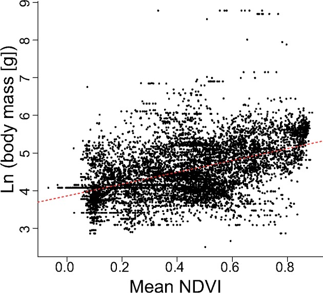
At the order-level, the PGLS analysis yielded a weak positive relationship between species-level body mass values and species-level NDVI values (P = 0.0020, b = 0.34, R²_adj = 0.007; Table 1a, Figure 1A), indicating larger rodent species in more productive habitats. PGLS analyses that consider uncertainty in species-level body mass values (i.e., the 1,000 randomized vectors) returned results (mean values and standard deviations) very similar to those of the empirical values (P = 0.0069 ± 0.0080, b = 0.34 ± 0.04, R²_adj = 0.005 ± 0.001; Supplementary Table S5, Figure 1A,B).

Table 1.

Summary of the PGLS analyses, where species-level body mass values (log body mass in grams) are being predicted by the species-level NDVI values (mean NDVI), at the order (a), suborder (b), and superfamily (c) levels

	df	b	F	R 2 adj	P
a. Order
Rodentia	1,299	0.34	9.45	0.007	0.0021
b. Suborder
Castorimorpha	77	0.80	3.31	0.029	0.0726
Hystricomorpha	181	0.15	0.28	0.000	0.5964
Myomorpha	817	0.41	9.74	0.011	0.0018
Sciuromorpha	205	0.41	1.86	0.004	0.1736
c. Superfamily
Dipodoidea	12	−0.71	0.49	−0.041	0.4991
Muroidea	803	0.42	9.91	0.011	0.0016

Significant P-values are in bold. Please note, results of taxa with low sample sizes (n < 10 or df < 8) are not shown. See “Materials and Methods” section for more information.

df, degrees of freedom (n − 2); b, coefficient estimate; F, F-statistic; R²_adj, adjusted R-squared value.

Figure 1.

Scatterplot of species-level NDVI values (unitless) versus species-level body mass values (grams) for order Rodentia (A). The red dashed line is the line of best fit based on the PGLS regression of the observed data (the points shown on the plot). The shaded blue area is the region occupied by the lines of best fit for each one of the 1,000 vectors of randomized log body mass values (the points are not shown on the plot). In (B), from top to bottom, a histogram showing the frequency distribution of the adjusted R² values of each randomized PGLS analysis, followed by a frequency distribution of the λ values estimated from the residuals of the regression model (using maximum likelihood), and the P-values for each randomized PGLS. The red vertical line indicates P = 0.05. Results of the empirical PGLS analysis are shown in Table 1 and those of the randomized PGLS analyses are found in Supplementary Table S5.

None of the examined suborders showed a significant association between species-level body mass and species-level NDVI values (all P ≥ 0.0726; Table 1b), except for Myomorpha, which showed a weak, significant, positive association between these variables (P = 0.0018, b = 0.41, R²_adj = 0.011; Table 1b). Of the 2 examined superfamilies, Muroidea showed a weak, significant, positive association between species-level body mass and species-level NDVI values (P = 0.0016, b = 0.42, R²_adj = 0.011), whereas Dipodoidea showed no significant association between these variables (P = 0.4991; Table 1c). At the family level, a significant positive association between species-level body mass and species-level NDVI values was found in Erethizontidae (P = 0.0132, b = 5.54, R²_adj = 0.457), Muridae (P = 0.0116, b = 0.64, R²_adj = 0.016), and Spalacidae (P = 0.0055, b = 3.82, R²_adj = 0.548; Table 2a)—all other examined families showed no significant association between these variables (all P ≥ 0.0613; Table 2a). Among examined subfamilies, a significant positive association between species-level body mass and species-level NDVI values was found in Gerbillinae (P = 0.0145, b = 1.54, R²_adj = 0.108), Neotominae (P = 0.0008, b = 0.92, R²_adj = 0.108), Xerinae (P = 0.0005, b = 1.20, R²_adj = 0.106), and Erethizontinae (P = 0.0206, b = 5.50, R²_adj = 0.447)—all other subfamilies showed no significant association between these variables (all P ≥ 0.0774; Table 2b). At the genus level, the association between species-level body mass and species-level NDVI values was significantly positive in Peromyscus (P = 0.0171, b = 0.77, R²_adj = 0.124) and Tamias (P = 0.0071, b = 0.957, R²_adj = 0.2534)—all other genera showed no significant association between these variables (all P ≥ 0.0705; Table 3).

Table 2.

Summary of the PGLS analyses, where species-level body mass values (log body mass in grams) are being predicted by the species-level NDVI values (mean NDVI), at the family (a) and subfamily (b) levels

	df	b	F	R 2 adj	P
a. Family
Bathyergidae	8	1.58	1.29	0.032	0.2872
Caviidae	11	−1.93	3.18	0.154	0.1017
Cricetidae	424	0.16	1.52	0.001	0.2182
Ctenomyidae	34	−0.32	0.61	0.000	0.4384
Dasyproctidae	9	−0.96	0.38	0.000	0.5504
Dipodidae	12	−0.71	0.49	0.000	0.4991
Echimyidae	58	0.41	0.51	0.000	0.4772
Erethizontidae	9	5.54	9.44	0.457	0.0132
Geomyidae	24	0.82	1.59	0.023	0.2184
Gliridae	10	0.09	0.00	0.000	0.9508
Heteromyidae	49	0.86	3.67	0.051	0.0613
Muridae	331	0.64	6.42	0.016	0.0116
Nesomyidae	32	0.86	0.87	0.000	0.3588
Sciuridae	192	0.44	2.01	0.005	0.1573
Spalacidae	9	3.82	13.12	0.548	0.0055
b. Subfamily
Arvicolinae	63	−0.53	1.58	0.009	0.2128
Callosciurinae	29	−0.91	0.96	0.000	0.3357
Caviinae	8	0.66	0.75	0.000	0.4114
Dendromurinae	9	0.32	0.04	0.000	0.8480
Deomyinae	14	0.53	0.79	0.000	0.3875
Dipodomyinae	17	0.48	0.26	0.000	0.6183
Echimyinae	17	1.29	2.54	0.078	0.1293
Erethizontinae	8	5.50	8.27	0.447	0.0206
Eumysopinae	33	−0.13	0.02	−0.030	0.8641
Gerbillinae	44	1.54	6.46	0.109	0.0146
Heteromyinae	9	2.44	2.59	0.137	0.1418
Murinae	259	0.48	2.66	0.006	0.1036
Neotominae	88	0.92	11.88	0.108	0.0008
Nesomyinae	12	1.45	0.80	0.016	0.3890
Otomyinae	8	0.22	0.32	0.000	0.5839
Perognathinae	19	0.55	2.15	0.054	0.1588
Sciurinae	53	−1.47	3.24	0.039	0.0774
Sigmodontinae	254	0.03	0.06	0.000	0.8047
Xerinae	101	1.20	13.10	0.106	0.0005

Significant P-values are in bold. Please note, results of taxa with low sample sizes (n < 10 or df < 8) are not shown. See “Materials and Methods” section for more information.

df, degrees of freedom (n − 2); b, coefficient estimate; F, F-statistic; R²_adj, adjusted R-squared value.

Table 3.

Summary of the PGLS analyses, where species-level body mass values (log body mass in grams) are being predicted by the species-level NDVI values (mean NDVI), at the genus taxonomic level

	df	b	F	R 2 adj	P
Akodon	31	0.24	0.71	0.000	0.4065
Chaetodipus	10	0.42	1.28	0.025	0.2835
Ctenomys	34	−0.32	0.61	0.000	0.4384
Dipodomys	15	−0.51	0.39	0.000	0.5413
Gerbillus	9	2.72	1.09	0.009	0.3242
Microtus	28	−0.86	3.25	0.072	0.0819
Mus	9	0.03	0.00	0.000	0.9627
Neotoma	13	0.43	2.45	0.094	0.1412
Oecomys	11	−0.15	0.04	0.000	0.8391
Oligoryzomys	11	−0.20	0.53	0.000	0.4815
Oxymycterus	9	−0.40	0.13	0.000	0.7212
Paraxerus	8	−3.45	1.52	0.005	0.2524
Peromyscus	36	0.77	6.24	0.124	0.0171
Phyllotis	10	0.25	0.14	0.000	0.7095
Proechimys	18	0.24	0.65	0.000	0.4302
Pseudomys	17	1.38	2.24	0.064	0.1520
Rattus	24	−0.52	0.65	0.000	0.4272
Reithrodontomys	15	0.62	1.95	0.056	0.1827
Rhipidomys	10	−1.20	2.95	0.150	0.1168
Sciurus	23	−1.11	3.60	0.098	0.0705
Spermophilus	27	0.81	1.55	0.019	0.2234
Tamias	22	0.96	8.95	0.257	0.0067
Thomasomys	22	0.48	1.49	0.021	0.2352

Significant P-values are in bold. Please note, results of taxa with low sample sizes (n < 10 or df < 8) are not shown. See “Materials and Methods” section for more information.

df, degrees of freedom (n − 2); b, coefficient estimate; F, F-statistic; R²_adj, adjusted R-squared value.

Cross-assemblage analysis

The rodent assemblage-level NDVI values seem to be greatest near the equator, and particularly in regions that broadly correspond to tropical rainforests, such as the Amazon Rainforest of South America, the Congo Rainforest of Central Africa, and the Rainforests of Southeast Asia (Figure 2). These values are lowest in regions that broadly correspond with deserts, such as the Saharan Desert and the Arabian Desert (Figure 2). Overall, there is low correspondence between the spatial distribution of the assemblage-level NDVI values (Figure 2) and the assemblage-level body mass values (Figure 3). The regions with the highest assemblage-level body mass values seem to be geographically clustered mostly in the Caribbean, and somewhat in scattered regions in the Americas, Asia, and Australia (Figure 3). The regions with the lowest assemblage-level body mass values are scattered in both desert and mesic regions (Figure 3).

Figure 2.

Map of the assemblage-level NDVI values. This map and the associated color scale depict the values of the actual 1.5-degree grid cells used in the cross-assemblage analysis (those in Supplementary Table S4). Negative NDVI values (close to zero) represent permanently snow-covered terrestrial habitats with no discernable vegetation. The white regions of the map denote missing data. The latitude and the longitude are indicated in the Y- and X-axes, respectively.

Figure 3.

Map of the assemblage-level body mass values (logged). This map and the associated color scale depict the values of the actual 1.5-degree grid cells used in the cross-assemblage analysis (those in Supplementary Table S4). The white regions of the map denote regions where none of the 1,301 species are present. The latitude and the longitude are indicated in the Y- and X-axes, respectively.

Out of the 11 examined GLS models of the association between assemblage-level body mass values and assemblage-level NDVI values, the exponential autocorrelation model based on the great-circle (haversine) distance fit the data best, receiving 98.8% of the total weight (ΔAIC = 0.00, wi = 0.988; Table 4). Based on this model, assemblage-level body mass values are not significantly predicted by the assemblage-level NDVI values (P = 0.3979). In contrast, both the OLS and the GLS regression analyses that do not consider spatial autocorrelation (which do not fit the data well) show a significant and strong correlation between these variables (both P < 0.0001, both b = 1.57, OLS R²_adj = 0.219; Figure 4). This result indicates that most of the apparent correlation between assemblage-level body mass values and assemblage-level NDVI values is an artifact of spatial autocorrelation.

Table 4.

Selection table of the fits of the GLS models of the association between assemblage-level body mass and assemblage-level NDVI values

	ln L	AIC	ΔAIC	wi
No spatial autocorrelation structure	−7504.1	15014.2	13952.2	<0.001
Exponential autocorrelation (Euclidean)	−726.9	1463.7	401.7	<0.001
Exponential autocorrelation (haversine)	−526.0	1062.0	0.0	0.988
Gaussian autocorrelation (Euclidean)	−1046.0	2102.0	1040.0	<0.001
Gaussian autocorrelation (haversine)	−962.3	1934.6	872.5	<0.001
Linear autocorrelation (Euclidean)	−1832.7	3675.5	2613.5	<0.001
Linear autocorrelation (haversine)	−1347.3	2704.7	1642.6	<0.001
Rational quadratics autocorrelation (Euclidean)	−808.2	1626.4	564.4	<0.001
Rational quadratics autocorrelation (haversine)	−682.2	1374.4	312.3	<0.001
Spherical autocorrelation (Euclidean)	−733.2	1476.4	414.3	<0.001
Spherical autocorrelation (haversine)	−530.4	1070.8	8.8	0.012

ln L, restricted log-likelihood score; ΔAIC fit relative to the model with the lowest AIC score (italicized). The best-fit model based on ΔAIC and Akaike weights (wi) are denoted in bold. The degrees of freedom (n − 2) for all models is 7,600 (n − 2).

Figure 4.

Scatterplot of assemblage-level NDVI values (unitless) versus assemblage-level body mass values (in grams). The red dashed line corresponds to the regression line of best fit. Each point corresponds to one of the 7,602 grids cells used in the regression models.

Discussion

Larger rodent species tend to occur in wet environments (Alhajeri and Steppan 2016), and at lower latitudes (Maestri et al. 2016). Terrestrial habitat productivity is associated with both increased precipitation (e.g., Yang et al. 2009; Zhou et al. 2009; Guo et al. 2012; this study) and decreased latitude (Gillman et al. 2015). This suggests that habitat productivity is an important predictor of body size in rodent species. Yet, our data do not support the “resource availability hypothesis” (Blackburn and Hawkins 2004) in rodents. The association between body mass and NDVI was weak across species (P = 0.0020, b = 0.34, R²_adj = 0.007; Table 1a, Figure 1A) and insignificant across assemblages (P = 0.3979). This suggests that resource availability is as poor a predictor of rodent body size as temperature (i.e., Bergmann’s rule) (e.g., Freckleton et al. 2003; Meiri and Dayan 2003; Alhajeri and Steppan 2016; Maestri et al. 2016).

The cross-assemblage approach assesses the relationship between climate and the assembly of communities (Feldman and Meiri 2014). Based on this, our data support the view that habitat productivity does not play a large role in the assembly of global rodent communities. If we do not consider spatial autocorrelation (i.e., OLS regression), habitat productivity explains 21.9% of the variation in assemblage body size (Figure 4). This argues for reexamining previous results that do not consider spatial autocorrelation. Further investigation is warranted considering that macroecology was founded on studies conducted at large scales (e.g., Brown and Maurer 1989; Brown 1995).

At the assemblage level, NDVI values (Figure 2) and body mass values (Figure 3) show different spatial distributions. This may lead to differences in associations between these variables across geographic regions (e.g., Meiri et al. 2004; Rodríguez et al. 2008; Berke et al. 2013). For example, the Caribbean has large values of both NDVI and body mass (Figures 2 and 3). This pattern may reflect support for the resource availability hypothesis in this region. Alternatively, the increased body mass in the Caribbean could be explained by the “island rule” (Foster 1964)—a common trend toward gigantism on islands. This interpretation is more plausible given that this region is dominated by large endemic rodents such as hutias (Nowak 1999), which could have evolved their large size in relative isolation. Yet, resource availability may explain the island rule, because it is only observed resource-rich islands (McNab 2010).

According to Feldman and Meiri (2014), the cross-species approach focuses on trait evolution. Thus, our data suggest that resource availability plays a minor role in the evolution of body size at the order-level (Table 1a, Figure 1A). Rodent clades may have contrasting macroevolutionary patterns, which may lead to a net signal of no association (see Cruz et al. 2005). The strength of the association between body mass and NDVI varied across the examined subtaxa (Tables 1–3); a pattern detected in other animals (e.g., Berke et al. 2013). Support for the resource availability hypothesis was generally stronger at narrower scales (Tables 2 and 3) than broader ones (Table 1). Bergmann’s rule shows similar scale-dependence (Cruz et al. 2005; Berke et al. 2013). A potential explanation is that species share more biological attributes at narrower scales. This may lead to concordant (i.e., additive) macroevolutionary patterns.

Among the strongest support for the resource availability hypothesis was found in Erethizontidae (New World porcupines and relatives) (P = 0.0132, b = 5.54, R²_adj = 0.457) and Spalacidae (Old World mole-rats and relatives) (P = 0.0055, b = 3.82, R²_adj = 0.548; Table 2a). At first glance, these 2 families seem to have little in common. For example, spalacids are subterranean whereas erethizontids are arboreal (Nowak 1999). Yet, on closer look, both these groups consist of species with a specialized niche. Traits associated with either niche may respond in the same direction under similar environmental pressures. For example, an association between body mass and habitat richness was found in crested porcupines (Lovari et al. 2013), a hystricid rodent (Old World porcupine) that shares a similar specialized niche. To directly test this hypothesis, the propensity for convergence needs to be compared among specialists and generalists.

Our results are generally concordant with prior studies at lower taxonomic scales. For example, Gerbillinae showed a significant positive association between body mass and NDVI (P = 0.0145, b = 1.54, R²_adj = 0.108; Table 2b). This result agrees Alhajeri et al. (2015) who found that gerbil species from less arid environments had larger cranial sizes, even after phylogenetic correction. Likewise, Peromyscus showed a significant positive association between body mass and NDVI (P = 0.0171, b = 0.77, R²_adj = 0.124; Table 3), which agrees with García-Mendoza et al. (2018), who found a similar association at the intraspecific level in Peromyscus melanotis.

In conclusion, at this broad spatio-taxonomic scale, rodent body size variation can neither be explained by Bergmann’s rule (e.g., Alhajeri and Steppan 2016; Maestri et al. 2016) nor resource availability (this study). Support for the resource availability hypothesis varied among subtaxa (Tables 1–3) and among geographic regions (Figures 2 and 3). This may indicate conflicting macroevolutionary signals, which may have reduced association between habitat productivity and body size at broad scales. As such, the resource availability hypothesis may only apply to some taxa at certain geographic contexts.

References

- Aitken AC, 1934. On least-squares and linear combinations of observations. Proc R Soc Edinb 55:42–48. [Google Scholar]
- Akaike H, 1974. A new look at the statistical model identification. IEEE Trans Automat Contr 19:716–723. [Google Scholar]
- Alhajeri BH, 2016. A phylogenetic test of the relationship between saltation and habitat openness in gerbils (Gerbillinae, Rodentia). Mammal Res 61:231–241. [Google Scholar]
- Alhajeri BH, 2018. Craniomandibular variation in the taxonomically problematic gerbil genus Gerbillus (Gerbillinae, Rodentia): assessing the influence of climate, geography, phylogeny, and size. J Mamm Evol 25:261–276. [Google Scholar]
- Alhajeri BH, Hunt OJ, Steppan SJ, 2015. Molecular systematics of gerbils and deomyines (Rodentia: Gerbillinae, Deomyinae) and a test of desert adaptation in the tympanic bulla. J Zool Syst Evol Res 53:312–330. [Google Scholar]
- Alhajeri BH, Steppan SJ, 2016. Association between climate and body size in rodents: a phylogenetic test of Bergmann’s rule. Mammalian Biology 81:219–225. [Google Scholar]
- Alhajeri BH, Steppan SJ, 2018a. A phylogenetic test of adaptation to deserts and aridity in skull and dental morphology across rodents. J Mammal 99:1197–1216. [Google Scholar]
- Alhajeri BH, Steppan SJ, 2018b. Community structure in ecological assemblages of desert rodents. Biol J Linn Soc 124:308–318. [Google Scholar]
- Alhajeri BH, Fourcade Y, 2019. High correlation between species-level environmental data estimates extracted from IUCN expert range maps and from GBIF occurrence data. J Biogeogr 46:1329–1341. [Google Scholar]
- Amori G, Milana G, Rotondo C, Luiselli L, 2015. Macro-ecological patterns of the endemic Afrosoricida and Rodentia of Madagascar. Hystrix It J Mammal 26:53–57. [Google Scholar]
- Bannari A, Morin D, Bonn F, Huete AR, 1995. A review of vegetation indices. Remote Sens Rev 13:95–120. [Google Scholar]
- Beck J, Ballesteros-Mejia L, Buchmann CM, Dengler J, Fritz SA. et al. , 2012. What’s on the horizon for macroecology? Ecography 35:673–683. [Google Scholar]
- Bergmann C, 1847. Über die Verhältnisse der Wärmeökonomie der Thiere zu ihrer Grösse. Göttinger Studien 3:595–708. [Google Scholar]
- Berke SK, Jablonski D, Krug AZ, Roy K, Tomasovych A, 2013. Beyond Bergmann’s rule: size-latitude relationships in marine Bivalvia world-wide. Glob Ecol Biogeogr 22:173–183. [Google Scholar]
- Bhandari AK, Kumar A, Singh GK, 2012. Feature extraction using normalized difference vegetation index (NDVI): a case study of jabalpur city. Procedia Technol 6:612–621. [Google Scholar]
- Bivand R, Lewin-Koh N, 2017. Maptools: Tools for Reading and Handling Spatial Objects R package version 0.9-2 [cited 2018 July 23]. Available from: https://CRAN.R-project.org/package=maptools/.
- Bivand R, Keitt T, Rowlingson B, 2018. rgdal: Bindings for the ‘Geospatial’ Data Abstraction Library R package version 1.3-3 [cited 2018 July 23]. Available from: https://CRAN.R-project.org/package=rgdal/.
- Blackburn TM, Hawkins BA, 2004. Bergmann’s rule and the mammal fauna of northern North America. Ecography 27:715–724. [Google Scholar]
- Blackburn TM, Gaston KJ, 2003. Macroecology: Concepts and Consequences. Cambridge: Cambridge University Press. [Google Scholar]
- Blackburn TM, Gaston KJ, Loder N, 1999. Geographic gradients in body size: a clarification of Bergmann’s rule. Divers Distrib 5:165–174. [Google Scholar]
- Bozdogan H, 1987. Model selection and Akaike’s Information Criterion (AIC): the general theory and its analytical extensions. Psychometrika 52:345–370. [Google Scholar]
- Brown JH, 1995. Macroecology. Chicago (IL: ): University of Chicago Press. [Google Scholar]
- Brown JH, Maurer BA, 1989. Macroecology: the division among species on of food and continents space. Science 243:1145–1150. [DOI] [PubMed] [Google Scholar]
- Burnham KP, Anderson DR, 2002. Model Selection and Multimodel Inference: A Practical Information-Theoretic Approach. New York: Springer. [Google Scholar]
- Cano ARG, Cantalapiedra JL, Álvarez-Sierra MÁ, Fernández MH, 2014. A macroecological glance at the structure of late Miocene rodent assemblages from Southwest Europe. Scientific Reports 4:1–8. [DOI] [PMC free article] [PubMed] [Google Scholar]
- Carotenuto F, Diniz-Filho JAF, Raia P, 2015. Space and time: the two dimensions of Artiodactyla body mass evolution. Palaeogeogr Palaeoclimatol Palaeoecol 437:18–25. [Google Scholar]
- Chamberlain S, Szoecs E, Foster Z, Arendsee Z, Boettiger C. et al. , 2018. taxize: Taxonomic Information from around the Web R package version 0.9.3 [cited 2018 July 23]. Available from: https://github.com/ropensci/taxize/.
- Chidodo DJ, 2017. Evaluation of Normalized Difference Vegetation Index of Common Vegetation Habitats for Monitoring Rodent Population and Outbreaks in Isimani, Tanzania [Master’s Thesis]. Morogoro, Tanzania: Sokoine University of Agriculture.
- Cruz FB, Fitzgerald LA, Espinoza RE, Schulte JA, 2005. The importance of phylogenetic scale in tests of Bergmann’s and Rapoport’s rules: lessons from a clade of South American lizards. J Evol Biol 18:1559–1574. [DOI] [PubMed] [Google Scholar]
- Daniel WW, 1990. Applied Nonparametric Statistics .Boston (MA: ): PWS-Kent. [Google Scholar]
- Detsch F, 2018. gimms: Download and Process GIMMS NDVI3g Data R package version 1.1.0 [cited 2018 June 27]. Available from: https://CRAN.R-project.org/package=gimms/
- Dormann CF, McPherson JM, Araújo BM, Bivand R, Bolliger J. et al. , 2007. Methods to account for spatial autocorrelation in the analysis of species distributional data: a review. Ecography 30:609–628. [Google Scholar]
- Fabre P-H, Hautier L, Dimitrov D, Douzery E, 2012. A glimpse on the pattern of rodent diversification: a phylogenetic approach. BMC Evol Biol 12:1–19. [DOI] [PMC free article] [PubMed] [Google Scholar]
- Feldman A, Meiri S, 2014. Australian snakes do not follow Bergmann’s rule. Evol Biol 41:327–335. [Google Scholar]
- Forstmeier W, Wagenmakers E-J, Parker TH, 2017. Detecting and avoiding likely false-positive findings: a practical guide. Biol Rev 92:1941–1968. [DOI] [PubMed] [Google Scholar]
- Foster JB, 1964. Evolution of mammals on islands. Nature 202:234–235. [Google Scholar]
- Freckleton RP, Harvey PH, Pagel M, 2003. Bergmann’s rule and body size in mammals. Am Nat 161:821–825. [DOI] [PubMed] [Google Scholar]
- Gamon JA, Huemmrich KF, Stone RS, Tweedie CE, 2013. Spatial and temporal variation in primary productivity (NDVI) of coastal Alaskan tundra: decreased vegetation growth following earlier snowmelt. Remote Sens Environ 129:144–153. [Google Scholar]
- Gao Q, Zhu W, Schwartz MW, Ganjurjav H, Wan Y. et al. , 2016. Climatic change controls productivity variation in global grasslands. Sci Rep 6:26958.. [DOI] [PMC free article] [PubMed] [Google Scholar]
- García-Mendoza DF, López-González C, Hortelano-Moncada Y, López-Wilchis R, Ortega J, 2018. Geographic cranial variation in Peromyscus melanotis (Rodentia: Cricetidae) is related to primary productivity. J Mammal 99:898–905. [Google Scholar]
- Gaston KJ, Blackburn TM, 2000. Pattern and Process in Macroecology. Malden (MA: ): Blackwell Science. [Google Scholar]
- Gillman LN, Wright SD, Cusens J, McBride PD, Malhi Y. et al. , 2015. Latitude, productivity and species richness. Glob Ecol Biogeogr 24:107–117. [Google Scholar]
- Guo Q, Hu Z, Li S, Li X, Sun X. et al. , 2012. Spatial variations in aboveground net primary productivity along a climate gradient in Eurasian temperate grassland: effects of mean annual precipitation and its seasonal distribution. Glob Chang Biol 18:3624–3631. [Google Scholar]
- Gohli J, Voje KL, 2016. An interspecific assessment of Bergmann’s rule in 22 mammalian families. BMC Evol Biol 16:222.. [DOI] [PMC free article] [PubMed] [Google Scholar]
- Harvey PH, Pagel MD, 1991. The Comparative Method in Evolutionary Biology .Oxford: Oxford University Press. [Google Scholar]
- Hijmans RJ, 2018. raster: Geographic Data Analysis and Modeling R package version 2.6-7 [cited 2018 June 27]. Available from: https://CRAN.R-project.org/package=raster/.
- Hijmans RJ, Cameron SE, Parra JL, Jones PG, Jarvis A, 2005. Very high resolution interpolated climate surfaces for global land areas. Int J Climatol 25:1965–1978. [Google Scholar]
- Holben BN, 1986. Characteristics of maximum-value composite images from temporal AVHRR data. Int J Remote Sens 7:1417–1434. [Google Scholar]
- Inman JW, 1835. Navigation and Nautical Astronomy: For the Use of British Seamen. London: C. and J. Rivington. [Google Scholar]
- ITIS, 2018. Integrated Taxonomic Information System [cited 2018 June 27]. Available from: http://www.itis.gov/.
- IUCN, 2015. The IUCN Red List of Threatened Species Version 2017-3 [cited 2018 June 27]. Available from: https://www.iucnredlist.org/.
- Jones KE, Bielby J, Cardillo M, Fritz SA, O'Dell J. et al. , 2009. PanTHERIA: a species-level database of life history, ecology, and geography of extant and recently extinct mammals. Ecology 90:2648. [Google Scholar]
- Kendall MG, 1938. A new measure of rank correlation. Biometrika 30:81–93. [Google Scholar]
- Leith H, Whittaker RH, 1975. Primary Productivity of the Biosphere. New York: Springer. [Google Scholar]
- Lovari S, Sforzi A, Mori E, 2013. Habitat richness affects home range size in a monogamous large rodent. Behav Process 99:42–46. [DOI] [PubMed] [Google Scholar]
- Maestri R, Luza AL, Barros LD, Hartz SM, Ferrari A. et al. , 2016. Geographical variation of body size in sigmodontine rodents depends on both environment and phylogenetic composition of communities. J Biogeogr 43:1192–1202. [Google Scholar]
- Maestri R, Luza AL, Barros LD, Hartz SM, Ferrari A. et al. , 2017. Geographical patterns of body mass distribution are robust even when inserting uncertainty in average estimates of species body mass. J Biogeogr 44:2678–2680. [Google Scholar]
- Mayr E, 1956. Geographical character gradients and climatic adaptation. Evolution 10:105–108. [Google Scholar]
- McNab BK, 2010. Geographic and temporal correlations of mammalian size reconsidered: a resource rule. Oecologia 164:13–23. [DOI] [PubMed] [Google Scholar]
- Medina AI, Martí DA, Bidau CJ, 2007. Subterranean rodents of the genus Ctenomys (Caviomorpha, Ctenomyidade) follow the converse to Bergmann’s rule. J Biogeogr 34:1439–1454. [Google Scholar]
- Meiri S, 2011. Bergmann’s rule: what’s in a name? Glob Ecol Biogeogr 20:203–207. [Google Scholar]
- Meiri S, Dayan T, 2003. On the validity of Bergmann’s rule. J Biogeogr 30:331–351. [Google Scholar]
- Meiri S, Dayan T, Simberloff D, 2004. Carnivores, biases and Bergmann’s rule. Biol J Linn Soc 81:579–588. [Google Scholar]
- Mori E, Ancillotto L, Lovari S, Russo D, Nerva L. et al. , 2019. Skull shape and Bergmann’s rule in mammals: hints from Old World porcupines. J Zool 308:47–55. [Google Scholar]
- Myneni RB, Hall F, Sellers P, Marshak A, 1995. The interpretation of spectral vegetation indexes. IEEE Trans Geosci Remote Sens 33:481–486. [Google Scholar]
- Nowak RM, 1999. Walker’s Mammals of the World. 6th edn Baltimore (MD: ): Johns Hopkins University Press. [Google Scholar]
- Orme D, Freckleton R, Thomas G, Petzoldt T, Fritz S. et al. , 2018. caper: Comparative Analyses of Phylogenetics and Evolution in R R package version 1.0.1 [cited 2018 June 27]. Available from: https://CRAN.R-project.org/package=caper/.
- Pabinger S, Rödiger S, Kriegner A, Vierlinger K, Weinhäusel A, 2014. A survey of tools for the analysis of quantitative PCR (qPCR) data. Biomol Detect Quantif 1:23–33. [DOI] [PMC free article] [PubMed] [Google Scholar]
- Pagel M, 1999. Inferring the historical patterns of biological evolution. Nature 401:877–884. [DOI] [PubMed] [Google Scholar]
- Pinheiro J, Bates D, DebRoy S, Sarkar D, R Core Team, 2017. nlme: Linear and Nonlinear Mixed Effects Models R package version 3.1-131 [cited 2018 April 26]. Available from: https://CRAN.R-project.org/package=nlme/.
- Pinzon EJ, Tucker JC, 2014. A non-stationary 1981–2012 AVHRR NDVI3g time series. Remote Sens 6:6929–6960. [Google Scholar]
- Riemer K, Guralnick RP, White EP, 2018. No general relationship between mass and temperature in endothermic species. Elife e27166:1–16. [DOI] [PMC free article] [PubMed] [Google Scholar]
- Rodríguez MA, Ollala-Tárraga MÁ, Hawkins BA, 2008. Bergmann’s rule and the geography of mammal body size in the Western Hemisphere. Glob Ecol Biogeogr 17:274–283. [Google Scholar]
- Saravanan S, Jegankumar R, Selvaraj A, Jacinth Jennifer J, Parthasarathy KSS, 2019. Utility of landsat data for assessing mangrove degradation in Muthupet Lagoon, South India In: Ramkumar M, James RA, Menier D, Kumaraswamy KBT, editors. Coastal Zone Management. Amsterdam, Netherlands: Elsevier; 471–484. [Google Scholar]
- Shelomi M, Zeuss D, 2017. Bergmann’s and Allen’s rules in native European and Mediterranean Phasmatodea. Front Ecol Evol 5:1–13. [Google Scholar]
- Smith FA, Lyons SK, 2011. How big should a mammal be? A macroecological look at mammalian body size over space and time. Philos Trans R Soc Lond B Biol Sci 366:2364–2378. [DOI] [PMC free article] [PubMed] [Google Scholar]
- R Development Core Team, 2018. A Language and Environment for Statistical Computing. Vienna, Austria: R Foundation for Statistical Computing [cited 2018 June 27]. Available from: https://www.R-project.org/.
- Rosenzweig ML, 1968. The strategy of body size in mammalian carnivores. Am Midl Nat 80:299–315. [Google Scholar]
- Taylor JM, Smith SC, Calaby JH, 1985. Altitudinal distribution and body size among New Guinean Rattus (Rodentia: Muridae). J Mammal 66:353–358. [Google Scholar]
- Vilela B, Villalobos F, 2015. Letsr: a new r package for data handling and analysis in macroecology. Methods Ecol Evol 6:1229–1234. [Google Scholar]
- Virgós E, Kowalczyk R, Trua A, de Marinis A, Mangas JG. et al. , 2011. Body size clines in the European badger and the abundant centre hypothesis. J Biogeogr 38:1546–1556. [Google Scholar]
- Wagenmakers EJ, Farrell S, 2004. AIC model selection using Akaike weights. Psychon Bull Rev 11:192–196. [DOI] [PubMed] [Google Scholar]
- Wilson DE, Reeder DM, 2005. Mammal Species of the World: A Taxonomic and Geographic Reference. Baltimore (MD: ): Johns Hopkins University Press. [Google Scholar]
- Yang YH, Fang JY, Pan YD, Ji CJ, 2009. Aboveground biomass in Tibetan grasslands. J Arid Environ 73:91–95. [Google Scholar]
- Yu X, Wu Z, Guo X, 2013. Investigating the potential of GIMMS and MODIS NDVI data sets for estimating gross primary productivity in Harvard Forest. In: MultiTemp 2013: 7th International Workshop on the Analysis of Multi-temporal Remote Sensing Images, Banff, AB, Canada. IEEE, pp. 1–4. doi: 10.1109/Multi-Temp.2013.6866013. [Google Scholar]
- Zhou X, Talley M, Luo Y, 2009. Biomass, litter, and soil respiration along a precipitation gradient in Southern Great Plains, USA. Ecosystems 12:1369–1380. [Google Scholar]
- Zhu Q, Zhao J, Zhu Z, Zhang H, Zhang Z. et al. , 2017. Remotely sensed estimation of net primary productivity (NPP) and its spatial and temporal variations in the Greater Khingan Mountain region, China. Sustainability 9:1213. [Google Scholar]
Associated Data
This section collects any data citations, data availability statements, or supplementary materials included in this article.
Supplementary Materials
Data Availability Statement
All macroecological environmental data generated for this study are available in the supporting information of this article.