

Abstract
This paper proposes a deep neural network (DNN) model using the reduced input feature space of Parkinson’s telemonitoring dataset to predict Parkinson’s disease (PD) progression. PD is a chronic and progressive nervous system disorder that affects body movement. PD is assessed by using the unified Parkinson’s disease rating scale (UPDRS). In this paper, firstly, principal component analysis (PCA) is employed to the featured dataset to address the multicollinearity problems in the dataset and to reduce the dimension of input feature space. Then, the reduced input feature space is fed into the proposed DNN model with a tuned parameter norm penalty (L2) and analyses the prediction performance of it in PD progression by predicting Motor and Total-UPDRS score. The model’s performance is evaluated by conducting several experiments and the result is compared with the result of previously developed methods on the same dataset. The model’s prediction accuracy is measured by fitness parameters, mean absolute error (MAE), root mean squared error (RMSE), and coefficient of determination (R2). The MAE, RMSE, and R2 values are 0.926, 1.422, and 0.970 respectively for motor-UPDRS. These values are 1.334, 2.221, and 0.956 respectively for Total-UPDRS. Both the Motor and Total-UPDRS score is better predicted by the proposed method. This paper shows the usefulness and efficacy of the proposed method for predicting the UPDRS score in PD progression.
Keywords: Deep neural network, Prediction, Parkinson disease progression, Principal component analysis
Introduction
PD [1] is a chronic and progressive nervous system disorder that affects movement. It is estimated that by 2020, approximately one million people will be living with PD in the U.S, which is more than those affected by Amyotrophic lateral sclerosis, Multiple sclerosis, and Muscular dystrophy combined. Also, worldwide, around 7–10 million people are living with PD [2]. The signs and symptoms of the disease include: tremor, slowed movement, rigid muscles, impaired posture and balance, loss of automatic movements, speech changes, and writing changes. Although the cause of the disease is unknown, researchers have identified specific genetic mutations and exposure to certain toxic as the cause of the disease [3]. Several scales have been developed for assessing the stage of PD [4]. UPDRS is the most commonly used scale for PD assessment [5]. The UPDRS is assessed by the following [6]: (i) assessment of behavior, mentation, and mood (ii) self-assessment of activities of daily life’s (ADLs) such as hygiene, speech, walking, handwriting, swallowing, dressing, falling, salivating, cutting food, and turning in bed (iii) motor assessment through clinicians monitoring (iv) therapy complications (v) severity of PD staging by Hoehn and Yahr (vi) ADL scale by Schwab and England. It has been observed that the scores for “mentation, behavior, and mood” increase later in the disease. However, other scores develop in the early-onset form of the disease [7]. Motor and Total-UPDRS refers respectively the motor section and full range of metric. Shulman et al. [8] had studied the clinically important difference on the UPDRS. Recognition of the PD is a challenge for the researchers, especially in the early stage as the cardinal features are not conclusive in this phase [9]. Early diagnosis of PD affects disease progression and the quality of life [10]. PD patient’s age plays a crucial role in PD progression, particularly, the older age is found to be related to more rapid motor impairment [11, 12]. The gender difference is also found to be associated with PD progression [13].
Many researchers have worked for the diagnosis of PD using machine learning (ML) techniques. Authors of [14, 15] have used support vector machine (SVM), authors of [16–19] have used neural network (NN), authors of [20, 21] have used fuzzy logic (FL), authors of [22] have used genetic programming (GP), authors of [23] have used random forest (RF), authors of [24] have used decision tree (DT), authors of [25] have used GP and expectation maximization (EM), authors of [26] have used KNN, FL, and K-means (KM), authors of [27] have used SVM and NN, authors of [28] have used SVM, KNN, FL, and Principal component analysis (PCA), authors of [29] have used NN, EM, PCA, and linear discriminant analysis (LDA), authors of [30] have used KNN, NN, and association rule (AR), authors of [31] have used SVM, KNN, and naïve Bayes (NB). Table 1 shows the various studies conducted on the automated diagnosis of PD.
Table 1.
Related work on PD diagnosis using different machine learning techniques [32]
| Authors | Techniques | ||||||||||||
|---|---|---|---|---|---|---|---|---|---|---|---|---|---|
| SVM | KNN | NN | FL | KM | GP | EM | PCA | RF | LDA | DT | AR | NB | |
| Bhattacharya and Bhatia [14] | ✓ | ||||||||||||
| Ozcift [15] | ✓ | ||||||||||||
| Das [16] | ✓ | ||||||||||||
| Babu and Suresh [17] | ✓ | ||||||||||||
| Buza and Varga [18] | ✓ | ||||||||||||
| Al-Fatlawi et al. [19] | ✓ | ||||||||||||
| Åström and Koker [20] | ✓ | ||||||||||||
| Li et al. [21] | ✓ | ||||||||||||
| Avci and Dogantekin [22] | ✓ | ||||||||||||
| Peterek et al. [23] | ✓ | ||||||||||||
| Froelich et al. [24] | ✓ | ||||||||||||
| Guo et al. [25] | ✓ | ✓ | |||||||||||
| Polat [26] | ✓ | ✓ | ✓ | ||||||||||
| Eskidere et al. [27] | ✓ | ✓ | |||||||||||
| Chen et al. [28] | ✓ | ✓ | ✓ | ✓ | |||||||||
| Hariharan et al. [29] | ✓ | ✓ | ✓ | ✓ | |||||||||
| Jain and Shetty [30] | ✓ | ✓ | ✓ | ||||||||||
| Behroozi and Sami [31] | ✓ | ✓ | ✓ | ||||||||||
In this paper, PCA is used with a deep learning paradigm for the assessment of PD progression. PCA addresses the multicollinearity problem in the data and reduces the dimensionality of the feature space that may improve the model’s performance. The deep learning paradigm provides numerous advantages over other ML techniques and has a great impact on state-of-the-art research in all domains of life including medical diagnosis and prognosis [33–35]. The deep networks can learn complex structures in high dimensional data. Moreover, unlike conventional ML algorithms, it does not require explicit feature extraction and selection [36]. This is done automatically by the deep networks. Not only it has beaten records in image recognition [37–39] and speech recognition [40–42], but also outperformed other ML techniques at predicting the activity of drug molecules [43], and predicting the effect of mutations in non-coding DNA on gene expression and disease [44, 45].
The rest of the paper is organized as follows. Section 2 briefly discusses the theoretical background of the model. Section 3 describes the dataset used. Section 4 describes the proposed DNN model. Section 5 presents the metric for the assessment of the model’s performance. Section 6 presents the finding of the proposed model and discussion about the results and implications of the current research. Finally, Sect. 7 concludes the paper.
Background
This section provides a brief discussion about the basic concepts of PCA and DNNs along with the hyperparameters tuning method used in the new DNN model proposed in this paper.
PCA
PCA is used to extract the features in a multivariate analysis where a large number of correlated variables are present. The primary benefit of employing PCA is that it addresses the problem of multicollinearity by transforming the input space into a set of variables that are uncorrelated with each other. These uncorrelated variables are called principal components (PCs). Usually, the first few PCs can capture most of the variations present in the dataset. The first principal component contains the maximum variability present in the data and each succeeding component contains as much of the remaining variability as possible. Therefore, the least important PCs can be dropped to reduce the dimensionality of the dataset while retaining the most valuable parts of all the variables [46]. PCA, first calculate a matrix that summarizes how the original variables are related to one another. Then, the matrix is broken into two components, ‘direction’ and ‘magnitude’ to know the direction and magnitude of the data. The axes of the original variable coordinate system are rotated to new axes. The new axes, called principal axes, are aligned with directions of the best fitting line along which the original variation is present. The first principal axis is the line of best fit because the sum of squares of the perpendicular distance from the original data points is minimum. The subsequent principal axis is always perpendicular to the previous principal axis [47].
Suppose, a set X that contains ‘p’ number of variables, X = (x1, x2, …, xp) affects the UPDRS score. PCA obtains the set of new variables ξ = (ξ1, ξ2, …, ξp) that is a linear function of input space but uncorrelated. These new variables are called PCs where PC1 contains the maximum variation present in the dataset that decreases subsequently from PC1 to PCp. The variance contribution of each PC is calculated as [48];
| 1 |
For orthogonal transformation, the following conditions are required.
| 2 |
| 3 |
Deep neural networks
Deep neural networks (DNNs) are artificial neural networks having multiple layers. These networks can be trained with a large amount of data to learn the representations of data with various levels of abstraction automatically. DNNs use a backpropagation algorithm to discover the complex structures in large datasets. The backpropagation algorithm uses the error (the difference between the system’s output and known expected output) to modify the internal weights of the network [49]. There are many variants of deep learning such as recurrent neural network, deep Boltzmann machine, deep belief network, convolution neural networks (ConvNets), deep autoencoder, and deep neural network [50]. Recently, ConvNets has been applied for many medical diagnosis problems that use biomedical signals and images for disease classification [33, 51–54]. ConvNets can also be used for regression problems where the goal is to predict continuous value rather than discrete classes [55].
During training, the input to the network is a set of labeled data, which has two parts, the first part has the information about the various attributes related to the concerned domain and the second part has the information about the belongingness to a particular label (or target). In a classification task, the set of labels are categorized into classes. However, in a regression task, labels are not categorized and can take any real value. For both tasks, after training, the loss function is computed which estimates the error between the model’s output and the known expected output (target). The DNNs consists of a large number of adjustable weights and labeled examples (typically hundreds of millions) to train the network. These weights are adjusted to improve the performance of the models.
For proper adjustment of the weight vector, the gradient vector is computed by the learning algorithm, which indicates the increase or decrease in error when the weight is increased slightly. The weight vector is modified in the reverse direction of the gradient vector. The average of the loss function for the entire training example looks like a hilly landscape in the high-dimensional space of weight vectors. At the minimum point, the average output error is the lowest.
There are many optimization techniques available to find a good set of weights. Stochastic gradient descent (SGD) is a commonly used algorithm that computes the output and error by using the input vector for a few examples. After this, the average gradient is computed for those examples to compute the weight. This process is iterated for many small training datasets until the average of the loss function stops reducing. SGD can quickly find a good set of weights [56]. After training the network, performance is measured on the test dataset to know the generalization ability of the network system. For the optimization of DNNs performance, many decisions need to be taken regarding the overall network architecture and parameters. These include a deeper vs wider network, choice of the number of neurons in the hidden layer, choice of activation function, choice of the optimizer, choice of batch size, epoch, and implementation of a mechanism to avoid overfitting and underfitting of the network.
Optimizer
Adam is an optimization algorithm [57] which was introduced after the stochastic gradient descent (SGD), adaptive gradient algorithm (AdaGrad) [58], root mean square propagation (RMSProp) [59], AdaDelta [60], and SGDNesterov. Adam can be used instead of the well-known classical SGD algorithm for updating the network weights iteratively in the training phase. The basic difference between classical SGD and Adam is that SGD does not change the learning rate during training, however, Adam uses the estimate of first and second moments of the gradients to compute individual adaptive learning rates for different network weights (parameters). ‘Adam’ combines the advantages of two other variants of SGD—AdaGrad, and RMSProp. In [57], the authors compared the performance of AdaGrad, RMSProp, SGDNesterov, AdaDelta, and Adam. Among these, the performance of ‘Adam’ was found better when applied to different algorithms and datasets. Also, the authors of [61–63] suggested ‘Adam’ as the default optimizer for deep learning applications.
Regularization
One of the most common problems in machine learning is to prevent the situation where the performance of an algorithm is good on the training dataset but poor with the unseen dataset (that is test dataset). This situation is termed as overfitting. The reason for poor performance with the unseen dataset is that the model learns too well the details and the noise from the training dataset. In such situations, training error decreases but the test error does not decrease. The techniques applied to the learning algorithms for reducing the generalization error (error with the test dataset but not the training error) are called regularization. Therefore, in the context of deep learning, regularization improves the model’s performance with the unseen dataset by penalizing the weight matrices of the nodes [64].
L2 & L1 regularizers
Many regularization approaches limit the capacity of models such as logistic regression, neural networks, or linear regression, by adding a parameter norm penalty to the loss function. L2 parameter norm penalty is most common and simplest and it is known as weight decay. The L2 regularization strategy derives the weight closer to the origin but not exactly zero. This is done by adding a regularization term to the loss function. For more detail on the L2 regularization see [65]. Due to the addition of the regularization term to the loss function, the value of weight matrices decreases because of the assumption that neural networks with smaller weight matrices can lead to simpler models. The regularization term in the case of L2 is given below as follows.
| 4 |
where λ is a regularization hyperparameter whose value is to be optimized for better performance. In the case of L1, the cost function is given by adding the following regularization term in the loss function. Here, the absolute value of the weight is penalized, and unlike L2 the weight may be reduced to zero. Therefore, it is useful when we want to compress our model, otherwise, L2 is preferred.
| 5 |
Dataset used
The proposed DNN model has been implemented on real-world public dataset taken from the machine learning repository provided by the University of California at Irvine (UCI). The dataset was created by Athanasios Tsanas and Max Little [66]. The patient’s data were acquired from 10 medical centers in the US with the help of a telemonitoring device that was developed by Intel Corporation. The voice measurements were captured automatically from the patient’s home for 6 months period. The columns of the data include subject number, age, gender, test time, Motor-UPDRS, Total-UPDRS, and the 16 biomedical voice measures. The rows consist of a total of 5875 voice measurements taken from 42 PD patients. Each row corresponds to one voice recording and there are about 200 recordings per patient. The Motor and Total-UPDRS scores are used by the clinicians for the PD symptom assessment. The UPDRS score is more variable and subjective. Figure 1 shows the variability of Motor and Total-UPDRS scores. The various attributes related to the dataset and their description have been listed in Table 2.
Fig. 1.

Variability of motor and total-UPDRS scores
Table 2.
Description of the features and UPDRS scores of the Parkinson’s telemonitoring dataset [27]
| Description | Feature label | Min | Max | Mean | SD |
|---|---|---|---|---|---|
| Clinician’s motor UPDRS score, linearly interpolated | Motor-UPDRS (baseline) | 6 | 36 | 19.42 | 8.12 |
| Motor-UPDRS (after 3 months) | 6 | 38 | 21.69 | 9.18 | |
| Motor-UPDRS (after 6 months) | 5 | 41 | 29.57 | 9.17 | |
| Clinician’s total UPDRS score, linearly interpolated | Total-UPDRS (baseline) | 8 | 54 | 26.39 | 10.8 |
| Total-UPDRS (after 3 months) | 7 | 55 | 29.36 | 11.82 | |
| Total-UPDRS (after 6 months) | 7 | 54 | 29.57 | 11.92 | |
| Several measures of variation in fundamental frequency | MDVP:Jitter (%) | 8E−4 | 0.1 | 0.006 | 0.006 |
| MDVP:Jitter (Abs) | 2E−6 | 4E−4 | 4E−5 | 3E−5 | |
| MDVP:Jitter:RAP | 3E−4 | 0.057 | 0.003 | 0.003 | |
| MDVP:Jitter:PPQ5 | 4E−4 | 0.069 | 0.003 | 0.004 | |
| Jitter:DDP | 10E−4 | 0.173 | 0.009 | 0.009 | |
| Several measures of variation in amplitude | MDVP:Shimmer | 0.003 | 0.269 | 0.034 | 0.026 |
| MDVP:Shimmer (dB) | 0.026 | 2.107 | 0.311 | 0.230 | |
| Shimmer:APQ3 | 0.002 | 0.163 | 0.017 | 0.013 | |
| Shimmer:APQ5 | 0.002 | 0.167 | 0.020 | 0.017 | |
| Shimmer:APQ11 | 0.003 | 0.276 | 0.028 | 0.020 | |
| Shimmer:DDA | 0.005 | 0.488 | 0.052 | 0.040 | |
| Two measures of the ratio of noise to tonal components in the voice | NHR | 3E−4 | 0.749 | 0.032 | 0.060 |
| HNR | 1.659 | 37.875 | 21.679 | 4.291 | |
| A nonlinear dynamical complexity measure | RPDE | 0.151 | 0.966 | 0.541 | 0.101 |
| The signal fractal scaling exponent | DFA | 0.514 | 0.866 | 0.653 | 0.071 |
| A nonlinear measure of fundamental frequency variation | PPE | 0.022 | 0.732 | 0.220 | 0.092 |
| Age of the PD subjects | Age | 36 | 85 | 64.80 | 8.82 |
| Sex of the PD subjects | Sex (Male, Female) | NA | |||
| Test duration of the PD subjects | Test_time | NA | |||
PCA is used for feature extraction and dimensionality reduction. The whole dataset contains a total of 19 attributes that include, 16 biomedical speech features, age, gender, and test time duration. The PCA is employed on the whole dataset to extract the variance present in the whole dataset. The first few PCs are selected that captures the sufficient variation present in the whole dataset for efficient performance. And, then the selected PCs are fed to the new DNN model. The previous methods used only the 16 speech features for predicting the UPDRS score [32, 67]. However, in this paper, PCA extracted the features from the whole dataset that include age, gender, and test time duration of the PD patients. Clinically, the age and gender affect the UPDRS score [11–13].
Proposed DNN model
The proposed DNN model consists of a stack of four dense layers. These multiple non-linear layers provide the network with the ability to find the non-linear structures in the dataset. The input to the model is 8 principal components (PCs) as shown in Fig. 2. The number of neurons in the dense layer-1, dense layer-2, dense layer-3, and the output dense layer-4 are 160, 80, 40 and 1 respectively. The values of the various hyperparameters are adjusted using trial and error method, which includes optimization method, activation function, the number of hidden layers, the number of neurons in each layer, L2-regularizer, batch size, and epoch.
Fig. 2.

The basic structure of the proposed DNN model
Figure 3 shows the process flow of the proposed DNN model. First, the raw PD dataset that consists of a total of 5875 rows and 19 columns is selected. After this, PCA is applied to the raw dataset to reduce the dimensionality of the dataset which gives 19 independent principal components (PCs) corresponding to the 19 columns. As the first few PCs were able to retain the maximum variability present in the data. The proposed DNN model uses the first 8 PCs which reduces the input dimensionality to 8. The cumulative proportion of variance captured by the eight PCs (PC1 to PC8) is 96.23%. The reduced dataset was split into a training dataset, test dataset, and validation dataset. The training dataset is used to fit the model parameters. However, the validation dataset is used to evaluate the trained model and tuning of model parameters, and then the loss function is evaluated. This process continues until the maximum number of epochs is reached. When the maximum number of epochs is reached, the final tuned DNN model is obtained. Finally, the test dataset is applied to the final tuned DNN model to get the model’s prediction.
Fig. 3.

Process flow of the proposed DNN model
Model performance assessment metric
To investigate the performance of the prediction model, three statistical evaluation metrics, mean absolute error (MAE), root mean square error (RMSE), and coefficient of determination (R2) have been used. The corresponding evaluation metrics are represented by Eqs. (6)–(8). These evaluation metrics were calculated using the ‘hydroGOF’ R package [68].
| 6 |
| 7 |
| 8 |
where are respectively the actual value, predicted value by the method, average of [y1, y2, …, yn], and n denotes the entire number of samples.
Results and discussion
In this study, the proposed DNN model was built in the ‘Python 3.6’ tool and executed on PC with 2 core Intel(R) Core (TM) i5-7200U CPU@2.50 GHz processors and 8 GB of RAM. The performance of the proposed DNN model is tuned by conducting the experiments several times.
The scheme for splitting the reduced dataset into a training dataset, validation dataset, and test dataset is as follows: First, the entire dataset was split into a training dataset and test dataset in a 90/10 ratio. And, then the training dataset is split into the training dataset and validation dataset in the ratio of 80/20. As there is a total of 5875 data points. So, after the splitting, corresponding data points in the training, validation and test sets are 4229, 1058, and 588 respectively. Table 3 summarizes the descriptions of the best hyperparameters value which are optimized for the proposed model.
Table 3.
Description of the hyperparameters
| Hyperparameters | Values |
|---|---|
| Optimizer | Adam |
| Activation function | ReLu |
| Loss function | Mean squared error (MSE) |
| Number of dense hidden layers with the respective number of neurons in each layer | 4 with 160, 80, 40, 1 |
| Regularization method used in layer-1, layer-2, and layer-3 and the value at each layer | L2 (0.0001) |
| Batch size | 8 |
| Epochs | 2000 |
The decision to choose the optimal number of PCs that are to be fed as input to the proposed DNN model is taken by running the model with five, six, seven, eight, and nine PCs as input that captures 86.71%, 90.91%, 94.67%, 96.23%, and 97.32% of the overall variation (present in the data) respectively. The best performance is obtained with the 8 PCs. Figure 4 shows the proportion of the variance captured by the PCs. The number of hidden layers and the number of respective neurons in each hidden layer in the proposed DNN model is decided by analyzing the prediction metrics (MAE, RMSE, and R2) for both the Motor and Total-UPDRS for the different number of dense layers. For the predictive model, the number of neurons in the last layer is always 1 and the goal is to minimize the errors (MAE and RMSE) and maximize the prediction metrics R2. To keep the model simple, in general, it is required to have a smaller number of neurons in the respective layers and the number of neurons in the succeeding layer should be half of the previous layer. The effect of varying the number of dense layers and the number of neurons in the dense layers for batch size eight is presented in Table 4. It is observed from Table 4 that when the number of dense layers is 2 and as the number of neurons in the layers is increased from (1, 20) to (320, 1), the R2 value increases. Where the DNN configuration (320, 1) is found with better prediction accuracy (R2 value). The MAE and RMSE values for both the Motor and Total-UPDRS are also decreased for the same configuration (Table 4). Thereafter, the number of dense layers is increased to 3, it is observed that the R2 value for the Motor-UPDRS is increased from 0.840 to 0.921 when the configuration is varied from (64, 32, 1) to (320, 160, 1). However, the R2 value for the Total-UPDRS score is decreased from 0.910 to 0.898 when the configuration is varied from (64, 32, 1) to (320, 160, 1). When the number of dense layers is increased to 4, it is observed that by increasing the number of neurons in the respective layers, the best performance concerning all the metrics (MAE, RMSE, and R2) is achieved for (160, 80, 40, 1) configuration. In this case, the MAE, RMSE, and R2 values are (0.926, 1.422, 0.970) and (1.334, 2.221, 0.956) respectively for the Motor and Total-UPDRS. However, for the same number of dense layers, the performance decreases on increasing the number of neurons in the respective layers (see configuration (200, 50, 25, 1) in Table 4). To verify whether the model’s performance is optimized for the configuration (160, 80, 40, 1), the number of dense layers is increased to 5 and the number of neurons in the respective layers is increased from (40, 20, 10, 6, 1) to (160, 80, 40, 20, 1). It is observed that the performance of the configuration (160, 80, 40, 1) is better than all the configurations of 5-dense layers. This verifies that the configuration (160, 80, 40, 1) is optimal.
Fig. 4.
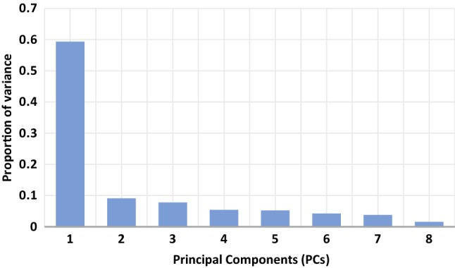
The proportion of the variance captured by PCs
Table 4.
Effect of varying the number of neurons in dense layers for batch size eight
| Number of dense layers | Number of neurons in the respective dense layers | Measure | MAE | RMSE | R2 |
|---|---|---|---|---|---|
| 2 | 20, 1 | Motor-UPDRS | 3.942 | 5.154 | 0.588 |
| Total-UPDRS | 4.954 | 6.511 | 0.619 | ||
| 80, 1 | Motor-UPDRS | 3.115 | 4.145 | 0.744 | |
| Total-UPDRS | 3.764 | 5.222 | 0.762 | ||
| 160, 1 | Motor-UPDRS | 3.117 | 4.325 | 0.719 | |
| Total-UPDRS | 3.993 | 5.350 | 0.749 | ||
| 320, 1 | Motor-UPDRS | 3.069 | 4.134 | 0.755 | |
| Total-UPDRS | 3.783 | 5.055 | 0.788 | ||
| 3 | 64, 32, 1 | Motor-UPDRS | 2.095 | 3.242 | 0.840 |
| Total-UPDRS | 2.030 | 3.181 | 0.910 | ||
| 160, 80, 1 | Motor-UPDRS | 1.531 | 2.570 | 0.898 | |
| Total-UPDRS | 1.727 | 2.813 | 0.931 | ||
| 320, 160, 1 | Motor-UPDRS | 1.399 | 2.242 | 0.921 | |
| Total-UPDRS | 2.167 | 3.378 | 0.898 | ||
| 4 | 32, 16, 8, 1 | Motor-UPDRS | 1.894 | 3.159 | 0.846 |
| Total-UPDRS | 1.770 | 2.604 | 0.938 | ||
| 64, 32, 16, 1 | Motor-UPDRS | 1.169 | 1.773 | 0.952 | |
| Total-UPDRS | 1.568 | 2.394 | 0.948 | ||
| 128, 64, 32, 1 | Motor-UPDRS | 1.069 | 1.959 | 0.942 | |
| Total-UPDRS | 1.462 | 2.657 | 0.940 | ||
| 160, 80, 40, 1 | Motor-UPDRS | 0.926 | 1.422 | 0.970 | |
| Total-UPDRS | 1.334 | 2.221 | 0.956 | ||
| 200, 100, 50, 1 | Motor-UPDRS | 1.399 | 2.324 | 0.915 | |
| Total-UPDRS | 1.415 | 2.383 | 0.954 | ||
| 5 | 40, 20, 10, 6, 1 | Motor-UPDRS | 1.298 | 2.002 | 0.938 |
| Total-UPDRS | 2.127 | 4.022 | 0.857 | ||
| 80, 40, 20, 10, 1 | Motor-UPDRS | 0.962 | 1.581 | 0.962 | |
| Total-UPDRS | 1.558 | 2.786 | 0.927 | ||
| 120, 60, 30, 16, 1 | Motor-UPDRS | 1.102 | 1.901 | 0.944 | |
| Total-UPDRS | 1.506 | 2.386 | 0.948 | ||
| 140, 70, 35, 18, 1 | Motor-UPDRS | 1.125 | 1.860 | 0.946 | |
| Total-UPDRS | 1.471 | 2.282 | 0.956 | ||
| 160, 80, 40, 20, 1 | Motor-UPDRS | 1.051 | 1.871 | 0.946 | |
| Total-UPDRS | 1.375 | 2.622 | 0.938 |
From, the number of experiments, it is found that the batch size for optimal performance is 8. To verify this, the batch size is varied from 4 to 24 while all the other hyperparameters values were kept the same as listed in Table 3. The effect of varying the batch size is presented in Table 5. It is observed from Table 5 that the best prediction performance is obtained for batch size 8 for both the Motor and Total-UPDRS. For batch size 4, the R2 value for Motor and Total-UPDRS is 0.954 and 0.935 respectively. However, for batch size 8, the R2 value for Motor and Total-UPDRS is 0.970 and 0.956 respectively which is the best. Further increase in the value of batch size does not improve the performance.
Table 5.
Effect of varying batch size
| Batch size | Measure | MAE | RMSE | R2 |
|---|---|---|---|---|
| 4 | Motor-UPDRS | 0.960 | 1.722 | 0.954 |
| Total-UPDRS | 1.688 | 2.826 | 0.935 | |
| 8 | Motor-UPDRS | 0.926 | 1.422 | 0.970 |
| Total-UPDRS | 1.334 | 2.221 | 0.956 | |
| 12 | Motor-UPDRS | 0.967 | 1.749 | 0.954 |
| Total-UPDRS | 1.469 | 2.540 | 0.944 | |
| 16 | Motor-UPDRS | 0.839 | 1.632 | 0.958 |
| Total-UPDRS | 1.823 | 2.755 | 0.942 | |
| 20 | Motor-UPDRS | 1.310 | 2.624 | 0.893 |
| Total-UPDRS | 1.397 | 2.576 | 0.940 | |
| 24 | Motor-UPDRS | 0.993 | 1.859 | 0.946 |
| Total-UPDRS | 1.315 | 2.314 | 0.952 |
Figure 5 shows the model’s convergence for the Motor and Total-UPDRS. It is observed from Fig. 5a that in the training phase of Motor-UPDRS, the model converges around 750 epochs. Also, the smooth convergence of the loss in the validation phase with the training phase indicates that the model has been tuned properly. In the case of Total-UPDRS, the model converges around 400 epochs as shown in Fig. 5b. Figure 6 depicts the scatter plot for the prediction of Motor-UPDRS and Total-UPDRS for the test dataset and validation dataset. The R2 values for the Motor-UPDRS in the test phase and validation phase are 0.970 and 0.948 respectively. The R2 values for the Total-UPDRS in the test phase and validation phase are 0.956 and 0.929 respectively. Figure 7 shows the prediction capability of the proposed DNN model for the Motor and Total-UPDRS. Figure 7a–c show the observed and predicted value of each data point in the training dataset, validation dataset, and test dataset respectively for the Motor-UPDRS. Similarly, Fig. 7d–f show the observed and predicted value of each data point in the training dataset, validation dataset, and test dataset respectively for the Total-UPDRS. Also, for Motor-UPDRS, the MAE, RMSE, and R2 values for the training phase, validation phase, and testing phase are found to be (0.783, 1.055, 0.984), (1.046, 1.949, 0.948), and (0.926, 1.422, 0.970) respectively in the order. However, for total-UPDRS, the MAE, RMSE, and R2 values for the training phase, validation phase, and testing phase are found to be (1.026, 1.398, 0.984), (1.520, 2.948, 0.929), and (1.334, 2.221, 0.956) respectively in the order.
Fig. 5.

Convergence curve for a motor-UPDRS and b total-UPDRS
Fig. 6.

Scatter plot for Motor-UPDRS in a test phase and b validation phase and Total-UPDRS in c test phase and d validation phase
Fig. 7.

Prediction capability of the DNN model for Motor-UPDRS a training phase, b validation phase, c testing phase, and total-UPDRS d training phase, e validation phase, f testing phase
To observe the effect of regularization parameter norm penalty (L2), the configuration (160, 80, 40, 1) is run with all the parameters the same as listed in Table 3 except that the L2 is not applied. In this case, the proposed DNN model overfits. This is verified by values of R2 in the training phase compared to values of R2 in the validation phase which is 0.998 and 0.855 respectively for Motor-UPDRS and 0.996 and 0.870 for Total-UPDRS. Therefore, L2 plays a crucial role in achieving better performance.
This paper compares the performance of the proposed DNN model with other methods [32, 67] for the prediction of Motor and Total-UPDRS which is shown in Table 6. Authors of [32, 67] normalize the observed Motor and Total-UPDRS values before predicting the MAE and RMSE values. This paper uses the original target values (which are numerically larger as compared to the normalized values) to predict MAE and RMSE values. This is why the predicted MAE and RMSE values are numerically larger than the previously proposed methods. From Table 6, it is observed that our method achieved the best R2 values for both the motor and total-UPDRS prediction which is 0.970 and 0.956 respectively for motor and total-UPDRS.
Table 6.
Results of MAE, RMSE, and R2 for all prediction methods
| Method | Measure | MAE | RMSE | R2 |
|---|---|---|---|---|
| MLR [32] | Motor-UPDRS | 0.997 | 2.4142 | 0.697 |
| Total-UPDRS | 0.987 | 2.3911 | 0.709 | |
| NN [32] | Motor-UPDRS | 0.977 | 2.3836 | 0.719 |
| Total-UPDRS | 0.951 | 2.3135 | 0.734 | |
| ANFIS [32] | Motor-UPDRS | 0.771 | 1.7047 | 0.785 |
| Total-UPDRS | 0.743 | 1.6062 | 0.798 | |
| SVR [32] | Motor-UPDRS | 0.721 | 1.4942 | 0.814 |
| Total-UPDRS | 0.689 | 1.4526 | 0.819 | |
| HSLSSVR [67] | Motor-UPDRS | – | 0.8158 | – |
| Total-UPDRS | – | 0.8004 | – | |
| SOM-NIPALS-ISVR [32] | Motor-UPDRS | 0.4656 | 0.6268 | 0.885 |
| Total-UPDRS | 0.4967 | 0.7097 | 0.868 | |
| PCA + Deep Learning (this study) | Motor-UPDRS | 0.926 | 1.422 | 0.970 |
| Total-UPDRS | 1.334 | 2.221 | 0.956 |
MLR multiple linear regression, NN neural network, ANFIS adaptive neuro-fuzzy inference system, SVR support vector regression, HSLSSVR householder transformation based sparse least squares support vector regression, SOM-NIPALS-ISVR self-organizing map-nonlinear iterative partial least squares-incremental support vector regression
The main findings of this study are that the deep learning-based prediction model is combined with PCA to enhance the performance of the PD prediction. The PCA produces as many principal components as the number of input features. But the first few PCs can capture the majority of the variations presents in the data. Also, all the PCs are independent of each other that solves the multicollinearity problem in the dataset. Therefore, the reduced and independent feature space (only 8 PCs) which is fed as input to the proposed DNN model results in a less complex DNN model that may improve the generalization capability of the proposed model. The proposed model achieved the best performance on the PD telemonitoring dataset compared to previously known methods. As the proposed DNN model is based on deep learning, the performance of the model may improve with the addition of more data points in datasets.
The proposed model is practical as the healthcare data tend to grow large. PCA extracted the features from the whole dataset that include age and gender of the PD patients. Clinically, the age and gender affect the UPDRS score [12, 13]. Therefore, the proposed method is more reliable and robust in predicting the UPDRS score.
Conclusion
This paper proposed a PCA based DNN model for the prediction of Motor-UPDRS and Total-UPDRS in PD progression. The DNN model was evaluated on a real-world PD dataset taken from UCI. It was observed that the proposed DNN model may precisely capture non-linearity in the feature space and shows better performance than the previously known methods, namely MLR, NN, ANFIS, SVR, HSLSSVR, and SOM-NIPALS-ISVR. Being a DNN model, the performance of the proposed model may improve with the addition of more data points in the datasets. PCA was used to extract the features from the whole dataset that include age and gender of the PD patients. Clinically, the age and gender affect the UPDRS score. Therefore, the proposed method is better, reliable, and robust in predicting the UPDRS score.
Acknowledgements
The authors would like to acknowledge the Ministry of Electronics & Information Technology (MeitY), Government of India for supporting the research work through “Visvesvaraya Ph.D. Scheme for Electronics & IT”.
Compliance with ethical standards
Conflict of interest
Afzal Hussain Shahid declares that he has no conflict of interest. Maheshwari Prasad Singh declares that he has no conflict of interest.
Ethical approval
This article does not contain any studies with human participants or animals performed by any of the authors.
Footnotes
Publisher's Note
Springer Nature remains neutral with regard to jurisdictional claims in published maps and institutional affiliations.
References
- 1.National Institute of Neurological Disorders and Stroke . Parkinson’s disease: hope through research. Bethesda: National Institute of Neurological Disorders and Stroke; 1994. [Google Scholar]
- 2.Marras C, Beck J, Bower J, Roberts E, Ritz B, Ross G, et al. Prevalence of Parkinson’s disease across North America. NPJ Parkinson’s Dis. 2018;4(1):21. doi: 10.1038/s41531-018-0058-0. [DOI] [PMC free article] [PubMed] [Google Scholar]
- 3.Clinic M. Parkinson’s disease (2019). https://www.mayoclinic.org.
- 4.Ramaker C, Marinus J, Stiggelbout AM, Van Hilten BJ. Systematic evaluation of rating scales for impairment and disability in Parkinson’s disease. Mov Disord. 2002;17(5):867–876. doi: 10.1002/mds.10248. [DOI] [PubMed] [Google Scholar]
- 5.Rascol O, Goetz C, Koller W, Poewe W, Sampaio C. Treatment interventions for Parkinson’s disease: an evidence based assessment. Lancet. 2002;359(9317):1589–1598. doi: 10.1016/S0140-6736(02)08520-3. [DOI] [PubMed] [Google Scholar]
- 6.Leon S, Mutnick H, Souney F, Swanson N. Comprehensive pharmacy review. Baltimore: West Camden Street; 2004. [Google Scholar]
- 7.Rosenbaum RB. Understanding Parkinson’s disease: a personal and professional view. Westport: Greenwood Publishing Group; 2006. [Google Scholar]
- 8.Shulman LM, Gruber-Baldini AL, Anderson KE, Fishman PS, Reich SG, Weiner WJ. The clinically important difference on the unified Parkinson’s disease rating scale. Arch Neurol. 2010;67(1):64–70. doi: 10.1001/archneurol.2009.295. [DOI] [PubMed] [Google Scholar]
- 9.Brooks DJ. The early diagnosis of Parkinson’s disease. Ann Neurol. 1998;44(1):S10–S18. doi: 10.1002/ana.410440704. [DOI] [PubMed] [Google Scholar]
- 10.Tsanas A, Little MA, McSharry PE, Ramig LO. Accurate telemonitoring of Parkinson’s disease progression by noninvasive speech tests. IEEE Trans Biomed Eng. 2010;57(4):884–893. doi: 10.1109/TBME.2009.2036000. [DOI] [PubMed] [Google Scholar]
- 11.Hely MA, Morris JG, Traficante R, Reid WG, O’Sullivan DJ, Williamson PM. The Sydney multicentre study of Parkinson’s disease: progression and mortality at 10 years. J Neurol Neurosurg Psychiatry. 1999;67(3):300–307. doi: 10.1136/jnnp.67.3.300. [DOI] [PMC free article] [PubMed] [Google Scholar]
- 12.Diamond S, Markham C, Hoehn M, McDowell F, Muenter M. Effect of age at onset on progression and mortality in Parkinson’s disease. Neurology. 1989;39(9):1187–1190. doi: 10.1212/wnl.39.9.1187. [DOI] [PubMed] [Google Scholar]
- 13.Haaxma CA, Bloem BR, Borm GF, Oyen WJ, Leenders KL, Eshuis S, et al. Gender differences in Parkinson’s disease. J Neurol Neurosurg Psychiatry. 2007;78(8):819–824. doi: 10.1136/jnnp.2006.103788. [DOI] [PMC free article] [PubMed] [Google Scholar]
- 14.Bhattacharya I, Bhatia MPS. SVM classification to distinguish Parkinson disease patients. In: Proceedings of the 1st Amrita ACM-W celebration on women in computing in India. ACM; 2010.
- 15.Ozcift A. SVM feature selection based rotation forest ensemble classifiers to improve computer-aided diagnosis of Parkinson disease. J Med Syst. 2012;36(4):2141–2147. doi: 10.1007/s10916-011-9678-1. [DOI] [PubMed] [Google Scholar]
- 16.Das R. A comparison of multiple classification methods for diagnosis of Parkinson disease. Expert Syst Appl. 2010;37(2):1568–1572. [Google Scholar]
- 17.Babu GS, Suresh S. Parkinson’s disease prediction using gene expression—a projection based learning meta-cognitive neural classifier approach. Expert Syst Appl. 2013;40(5):1519–1529. [Google Scholar]
- 18.Buza K, Varga NÁ. ParkinsoNET: estimation of UPDRS score using hubness-aware feedforward neural networks. Applied Artificial Intelligence. 2016;30(6):541–555. [Google Scholar]
- 19.Al-Fatlawi AH, Jabardi MH, Ling SH. Efficient diagnosis system for Parkinson’s disease using deep belief network. In: 2016 IEEE congress on evolutionary computation (CEC). IEEE; 2016.
- 20.Åström F, Koker R. A parallel neural network approach to prediction of Parkinson’s disease. Expert Syst Appl. 2011;38(10):12470–12474. [Google Scholar]
- 21.Li D-C, Liu C-W, Hu SC. A fuzzy-based data transformation for feature extraction to increase classification performance with small medical data sets. Artif Intell Med. 2011;52(1):45–52. doi: 10.1016/j.artmed.2011.02.001. [DOI] [PubMed] [Google Scholar]
- 22.Avci D, Dogantekin A. An expert diagnosis system for parkinson disease based on genetic algorithm-wavelet kernel-extreme learning machine. Parkinson’s Dis. 2016;2016:5264743. doi: 10.1155/2016/5264743. [DOI] [PMC free article] [PubMed] [Google Scholar]
- 23.Peterek T, Dohnálek P, Gajdoš P, Šmondrk M. Performance evaluation of Random Forest regression model in tracking Parkinson’s disease progress. In: 13th international conference on hybrid intelligent systems (HIS 2013). IEEE; 2013.
- 24.Froelich W, Wrobel K, Porwik P. Diagnosis of Parkinson’s disease using speech samples and threshold-based classification. J Med Imaging Health Inform. 2015;5(6):1358–1363. [Google Scholar]
- 25.Guo P-F, Bhattacharya P, Kharma N. Advances in detecting Parkinson’s disease. In: International conference on medical biometrics. Springer; 2010.
- 26.Polat K. Classification of Parkinson’s disease using feature weighting method on the basis of fuzzy C-means clustering. Int J Syst Sci. 2012;43(4):597–609. [Google Scholar]
- 27.Eskidere Ö, Ertaş F, Hanilçi C. A comparison of regression methods for remote tracking of Parkinson’s disease progression. Expert Syst Appl. 2012;39(5):5523–5528. [Google Scholar]
- 28.Chen H-L, Huang C-C, Yu X-G, Xu X, Sun X, Wang G, et al. An efficient diagnosis system for detection of Parkinson’s disease using fuzzy k-nearest neighbor approach. Expert Syst Appl. 2013;40(1):263–271. [Google Scholar]
- 29.Hariharan M, Polat K, Sindhu R. A new hybrid intelligent system for accurate detection of Parkinson’s disease. Comput Methods Programs Biomed. 2014;113(3):904–913. doi: 10.1016/j.cmpb.2014.01.004. [DOI] [PubMed] [Google Scholar]
- 30.Jain S, Shetty S. Improving accuracy in noninvasive telemonitoring of progression of Parkinson’s disease using two-step predictive model. In: Third international conference on electrical, electronics, computer engineering and their applications (EECEA). IEEE; 2016.
- 31.Behroozi M, Sami A. A multiple-classifier framework for Parkinson’s disease detection based on various vocal tests. Int J Telemed Appl. 2016 doi: 10.1155/2016/6837498. [DOI] [PMC free article] [PubMed] [Google Scholar]
- 32.Nilashi M, Ibrahim O, Ahmadi H, Shahmoradi L, Farahmand M. A hybrid intelligent system for the prediction of Parkinson’s disease progression using machine learning techniques. Biocybern Biomed Eng. 2018;38(1):1–15. [Google Scholar]
- 33.Acharya UR, Oh SL, Hagiwara Y, Tan JH, Adeli H. Deep convolutional neural network for the automated detection and diagnosis of seizure using EEG signals. Comput Biol Med. 2018;100:270–278. doi: 10.1016/j.compbiomed.2017.09.017. [DOI] [PubMed] [Google Scholar]
- 34.Yu L, Chen H, Dou Q, Qin J, Heng P-A. Automated melanoma recognition in dermoscopy images via very deep residual networks. IEEE Trans Med Imaging. 2017;36(4):994–1004. doi: 10.1109/TMI.2016.2642839. [DOI] [PubMed] [Google Scholar]
- 35.Liu M, Zhang J, Adeli E, Shen D. Landmark-based deep multi-instance learning for brain disease diagnosis. Med Image Anal. 2018;43:157–168. doi: 10.1016/j.media.2017.10.005. [DOI] [PMC free article] [PubMed] [Google Scholar]
- 36.Shahid AH, Singh MP. Computational intelligence techniques for medical diagnosis and prognosis: problems and current developments. Biocybern Biomed Eng. 2019;10(3):345. [Google Scholar]
- 37.Krizhevsky A, Sutskever I, Hinton GE. Imagenet classification with deep convolutional neural networks. Advances in neural information processing systems. Red Hook: Curran Associates Inc.; 2012. [Google Scholar]
- 38.Farabet C, Couprie C, Najman L, LeCun Y. Learning hierarchical features for scene labeling. IEEE Trans Pattern Anal Mach Intell. 2013;35(8):1915–1929. doi: 10.1109/TPAMI.2012.231. [DOI] [PubMed] [Google Scholar]
- 39.Szegedy C, Liu W, Jia Y, Sermanet P, Reed S, Anguelov D, et al. Going deeper with convolutions. In: Proceedings of the IEEE conference on computer vision and pattern recognition; 2015.
- 40.Mikolov T, Deoras A, Povey D, Burget L, Černocký J. Strategies for training large scale neural network language models. In: IEEE workshop on automatic speech recognition and understanding (ASRU). IEEE; 2011.
- 41.Hinton G, Deng L, Yu D, Dahl GE, Mohamed A-R, Jaitly N, et al. Deep neural networks for acoustic modeling in speech recognition: the shared views of four research groups. IEEE Signal Process Mag. 2012;29(6):82–97. [Google Scholar]
- 42.Sainath TN, Mohamed A-R, Kingsbury B, Ramabhadran B. Deep convolutional neural networks for LVCSR. In: 2013 IEEE international conference on acoustics, speech and signal processing (ICASSP). IEEE; 2013.
- 43.Ma J, Sheridan RP, Liaw A, Dahl GE, Svetnik V. Deep neural nets as a method for quantitative structure–activity relationships. J Chem Inf Model. 2015;55(2):263–274. doi: 10.1021/ci500747n. [DOI] [PubMed] [Google Scholar]
- 44.Leung MK, Xiong HY, Lee LJ, Frey BJ. Deep learning of the tissue-regulated splicing code. Bioinformatics. 2014;30(12):i121–i129. doi: 10.1093/bioinformatics/btu277. [DOI] [PMC free article] [PubMed] [Google Scholar]
- 45.Xiong HY, Alipanahi B, Lee LJ, Bretschneider H, Merico D, Yuen RK, et al. The human splicing code reveals new insights into the genetic determinants of disease. Science. 2015;347(6218):1254806. doi: 10.1126/science.1254806. [DOI] [PMC free article] [PubMed] [Google Scholar]
- 46.Jolliffe I. Principal component analysis. In: Lorvic M, editor. International encyclopedia of statistical science. New York: Springer; 2011. pp. 1094–1096. [Google Scholar]
- 47.Campbell N, Atchley WR. The geometry of canonical variate analysis. Syst Biol. 1981;30(3):268–280. [Google Scholar]
- 48.Hu T, Wu F, Zhang X. Rainfall–runoff modeling using principal component analysis and neural network. Hydrology Research. 2007;38(3):235–248. [Google Scholar]
- 49.LeCun Y, Bengio Y, Hinton G. Deep learning. Nature. 2015;521(7553):436. doi: 10.1038/nature14539. [DOI] [PubMed] [Google Scholar]
- 50.Ravı D, Wong C, Deligianni F, Berthelot M, Andreu-Perez J, Lo B, et al. Deep learning for health informatics. IEEE J Biomed Health Inform. 2017;21(1):4–21. doi: 10.1109/JBHI.2016.2636665. [DOI] [PubMed] [Google Scholar]
- 51.Acharya UR, Fujita H, Oh SL, Raghavendra U, Tan JH, Adam M, et al. Automated identification of shockable and non-shockable life-threatening ventricular arrhythmias using convolutional neural network. Fut Gener Comput Syst. 2018;79:952–959. [Google Scholar]
- 52.Acharya UR, Fujita H, Lih OS, Adam M, Tan JH, Chua CK. Automated detection of coronary artery disease using different durations of ECG segments with convolutional neural network. Knowl-Based Syst. 2017;132:62–71. [Google Scholar]
- 53.Tajbakhsh N, Shin JY, Gurudu SR, Hurst RT, Kendall CB, Gotway MB, et al. Convolutional neural networks for medical image analysis: full training or fine tuning? IEEE Trans Med Imaging. 2016;35(5):1299–1312. doi: 10.1109/TMI.2016.2535302. [DOI] [PubMed] [Google Scholar]
- 54.Kallenberg M, Petersen K, Nielsen M, Ng AY, Diao P, Igel C, et al. Unsupervised deep learning applied to breast density segmentation and mammographic risk scoring. IEEE Trans Med Imaging. 2016;35(5):1322–1331. doi: 10.1109/TMI.2016.2532122. [DOI] [PubMed] [Google Scholar]
- 55.Belagiannis V, Rupprecht C, Carneiro G, Navab N. Robust optimization for deep regression. In: Proceedings of the IEEE international conference on computer vision, 2015.
- 56.Bottou L, Bousquet O. The tradeoffs of large scale learning. Adv Neural Inf Process Syst. 2008;20:161–168. [Google Scholar]
- 57.Kingma DP, Ba JA. A method for stochastic optimization. arXiv preprint, 2014. arXiv:14126980.
- 58.Duchi J, Hazan E, Singer Y. Adaptive subgradient methods for online learning and stochastic optimization. J Mach Learn Res. 2011;12:2121–2159. [Google Scholar]
- 59.Tieleman T, Hinton G. Lecture 6.5-rmsprop: divide the gradient by a running average of its recent magnitude. COURSERA Neural Netw Mach Learn. 2012;4(2):26–31. [Google Scholar]
- 60.Zeiler MD. ADADELTA: an adaptive learning rate method. arXiv preprint, 2012. arXiv:12125701.
- 61.Karpathy A. Cs231n convolutional neural networks for visual recognition. Neural Netw. 2016;1:1. [Google Scholar]
- 62.Xu K, Ba J, Kiros R, Cho K, Courville A, Salakhudinov R, et al. Show, attend and tell: neural image caption generation with visual attention. In: International conference on machine learning, 2015.
- 63.Gregor K, Danihelka I, Graves A, Rezende DJ, Wierstra D. Draw: a recurrent neural network for image generation. arXiv preprint, 2015. arXiv:150204623.
- 64.Bühlmann P, Van De Geer S. Statistics for high-dimensional data: methods, theory and applications. Berlin: Springer; 2011. [Google Scholar]
- 65.Goodfellow I, Bengio Y, Courville A, Bengio Y. Deep learning. Cambridge: MIT Press; 2016. [Google Scholar]
- 66.Tsanas A, Little MA, McSharry PE, Ramig LO. Accurate telemonitoring of Parkinson’s disease progression by noninvasive speech tests. IEEE Trans Biomed Eng. 2009;57(4):884–893. doi: 10.1109/TBME.2009.2036000. [DOI] [PubMed] [Google Scholar]
- 67.Zhao Y-P, Li B, Li Y-B, Wang K-K. Householder transformation based sparse least squares support vector regression. Neurocomputing. 2015;161:243–253. [Google Scholar]
- 68.Bigiarini MZ, Bigiarini MMZ. Package “hydroGOF”. R-package www.r-project.org (2013). Accessed 7 May 2018.