Figure 5. Two-level Hierarchical Gaussian Filter for continuous inputs.

(A) Schematic of the two-level HGF, which models how an agent infers a hidden state in the environment (a random variable), $x_1$, as well as its rate of change over time ($x_2$, environmental volatility). Beliefs about those two hierarchically related hidden states ($x_1$, $x_2$) at trial $k$ are updated by the sensory input ($u^k$, observed feedback scores in our study) for that trial via prediction errors (PEs). The states $x_1$ and $x_2$ are continuous variables evolving as coupled Gaussian random walks, where the step size (variance) of the random walk depends on a set of parameters (shown in yellow boxes). The lowest level is coupled to the level above through the variance of the random walk: $x_1^k\sim 𝒩(x_1^{k-1},\exp (\kappa x_2^{k-1}+{\omega }_1))$. The posterior distribution of beliefs about these states is fully determined by the sufficient statistics ${\displaystyle {\mu }_i}$ (mean) and ${\displaystyle {\sigma }_i}$ (variance) for levels $i=1,2$. The equations describing how expectations (${\displaystyle {\mu }_i}$) change from trial $k-1$ to $k$ are Equation 6 and Equation 10. The response model generates the most probable response, $y^k$, according to the current beliefs, and is modulated by the response model parameters ${\beta }_0,{\beta }_1,{\beta }_2,\zeta$. In the winning model, the response parameter was the change between trial $k-1$ and $k$ in the degree of temporal variability across keystrokes: ${\displaystyle y^k=\mathrm{\Delta }\mathrm{c}\mathrm{v}\mathrm{I}\mathrm{K}{\mathrm{I}}_{\mathrm{t}\mathrm{r}\mathrm{i}\mathrm{a}\mathrm{l}}^{\mathrm{k}}}$, normalized to range 0–1. (B, C) Example of belief trajectories (mean, variance) associated with the two levels of the HGF for continuous inputs. Panel (C) displays the expectation on the first level, ${\mu }_1^k$, which represents an individual’s expectation (posterior mean) of the true reward values for the trial, $x_1^k$. Black dots represent the trial-wise input (feedback scores, $u^k$). Panel (B) shows the trial-by-trial beliefs about log-volatility $x_2^k$ , determined by the expectation ${\mu }_2^k$ and associated variance. Shaded areas denote the variance or estimation uncertainty on that level. (D) Illustration of the performance measure used as response in the winning model, ${\displaystyle y^k=\mathrm{\Delta }\mathrm{c}\mathrm{v}\mathrm{I}\mathrm{K}{\mathrm{I}}_{\mathrm{t}\mathrm{r}\mathrm{i}\mathrm{a}\mathrm{l}}^{\mathrm{k}}}$.

Figure 5—figure supplement 1. Trial-by-trial belief trajectories for simulated performances.

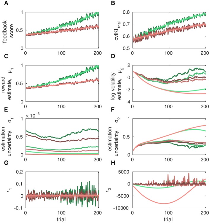
All belief trajectories were generated using prior values on the HGF parameters as shown in Table 1. We simulated performances in six agents by changing the trial-to-trial difference in IKI values across keystroke positions, thus leading to different trajectories of ${\mathrm{cvIKI}}_{\mathrm{trial}}$ (B) and feedback scores (A). We started with a pattern of IKI values of [0.2, 0.6, 0.2, 0.6, 0.2, 0.6, 0.2] s and iteratively prolonged the inter-keystroke interval at positions 2, 4, and 6, thereby increasing the temporal difference between IKI values, the vector norm of the total IKI pattern, and the cvIKI value across keystroke positions within the trial, termed ${\mathrm{cvIKI}}_{\mathrm{trial}}$. In the plot, steeper and shallower slopes of change across trials in ${\mathrm{cvIKI}}_{\mathrm{trial}}$ and associated feedback scores are denoted by green and pink colored lines, respectively. In addition, lighter colors denote smoother trial-by-trial transitions in ${\mathrm{cvIKI}}_{\mathrm{trial}}$ values. Darker colors indicate noisier trial-by-trial changes in this measure, representing an agent with a more variable behavioral strategy every trial. (C, D) Expectation on reward and log-volatility, and (E, F) the associated variance or estimation uncertainty. (G,H) Precision-weighted prediction error on reward, ${ϵ}_1$, and volatility, ${ϵ}_2$. A steeper slope of change in feedback scores and ${\mathrm{cvIKI}}_{\mathrm{trial}}$ was associated with higher log-volatility estimates and reduced uncertainty about volatility, ${\sigma }_2$. For a fixed slope, increasing levels of noise in the trajectories of the feedback scores and ${\mathrm{cvIKI}}_{\mathrm{trial}}$ also contributed to higher volatility estimates and reduced ${\sigma }_2$. Thus, agents either (i) introducing more fluctuations in behavior from trial to trial or (ii) observing a faster rise in scores had a higher expectation of volatility and lower uncertainty about volatility.

Figure 5—figure supplement 2. Simulated trial-by-trial belief trajectories in an ideal learner.

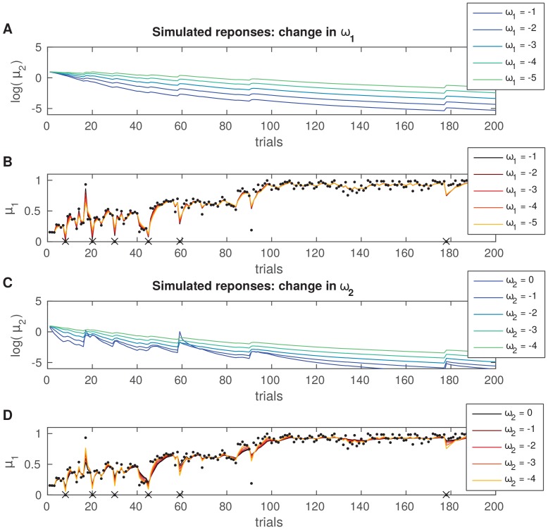
Simulated trial-by-trialtrajectories of posterior means of belief distributions in an ideal learner with different values of ${\omega }_1$ (A, B) or ${\omega }_2$ (C, D). All trajectories were simulated with identical input scores and parameters, except for ${\omega }_1$ (A, B) or ${\omega }_2$ (C, D): ${\mu }_1(0)=0.1,{\mu }_2(0)=1,{\sigma }_1(0)={\sigma }_2(0)=log(1),\kappa =1,{\pi }_u=1/35$ (precision of input). (A) Increasing values of ${\omega }_1$ (largest value ${\omega }_1$ = −1 in this example) lead to a more pronounced general reduction in the estimate of log-volatility across trials, log(${\mu }_2$). (B) The time series of the expectation on reward does not vary in a noticeable way as a function of ${\omega }_1$. (C) Increasing values of ${\omega }_2$ (largest value ${\omega }_2$ = 0 in this example) triggered more phasic trial-by-trial changes in the log-volatility estimate, log(${\mu }_2$), in response to prediction errors at the lower level (PE about reward, indicated by sharp changes in the trajectories of reward expectations in panel [D]). Increasing values of ${\omega }_2$ correspond to higher uncertainty in the prediction on that level (see Equation 13 in 'Materials and methods'). (D) Same as panel (B), but for varying values of ${\omega }_2$. Expectations on reward did not change considerably as a function of ${\omega }_2$ in this example.

Figure 5—figure supplement 3. $\beta$ coefficients of the winning response model.

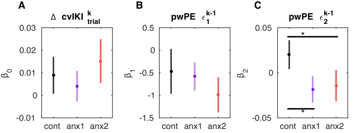
(A–C) Mean (and SEM) values of the $\beta$ coefficients that explain the performance measure in trial $k$ as a linear function of (i) a constant value ($\mathrm{\Delta }{\mathrm{cvIKI}}_{\mathrm{trial}}^{\mathrm{k}}$) and (ii) the precision-weighted prediction errors on the previous trial $k-1$: pwPE concerning reward (${ϵ}_1^{k-1}$) and pwPE concerning volatility (${ϵ}_2^{k-1}$). The performance measure in the winning model, $\mathrm{\Delta }{\mathrm{cvIKI}}_{\mathrm{trial}}^{\mathrm{k}}$, was the change in the degree of temporal variability across keystroke positions from trial $k-1$ to $k$. The $\beta$ values are plotted separately for each control and experimental group. The best response model was obtained using Random Effects Bayesian Model Comparison (BMC) in a set of two families of response models, followed by BMC within the winning family (see main text). The noise parameter $\zeta$ did not significantly differ between groups ($P>0.05$), and therefore we found no differences in how the model was able to estimate predicted responses to fit the observed responses in each group. (B, C) There were no significant between-group differences in ${\beta }_0$ or ${\beta }_1$ coefficients ($P>0.05$). (C) Control participants had a positive and significantly higher ${\beta }_2$ coefficient than anx1 and anx2 participants ($P_{FDR}<0.05$, denoted by the horizontal lines and black asterisks). This implies that in control participants an increase in ${ϵ}_2$ (larger update in the expectation of volatility) contributed to a greater change in the relevant performance measure on the following trial, yet it led to a decrease in anx1 and anx2.

Figure 5—figure supplement 4. Example in one control participant of the association between pwPEs and performance.

Example in one control participant of the association between pwPEs relating to volatility and subsequent changes in performance. (A, B) Illustration of the trajectory of pwPE relating to volatility on trial $k-1$, ${ϵ}_2^{k-1}$. Right panels are an enlarged display of a section of the corresponding left panel. (C, D) Trajectory of the expectation on log-volatility, ${\mu }_2^{k-1}$. (E, F) Performance measure in the winning response model, $\mathrm{\Delta }{\mathrm{cvIKI}}_{\mathrm{trial}}^{\mathrm{k}}$, representing the change from trial $k-1$ to $k$ in the task-relevant performance variable associated with reward, ${\mathrm{cvIKI}}_{\mathrm{trial}}^{\mathrm{k}}$. Green circles denote trials of large values of ${ϵ}_2$ that were followed by an increment in the performance measure (larger behavioral change). This figure illustrates the effect of positive ${\displaystyle {\beta }_2}$ coefficients in the response model in control participants, linking large ${\displaystyle {ϵ}_2}$ values to large changes in behavior on the next trial. Red circles mark trials of large ${ϵ}_2$ values that led to smaller changes in the performance variable in the subsequent trial.

Figure 5—figure supplement 5. Example in one anx1 participant of the association between pwPEs and performance.

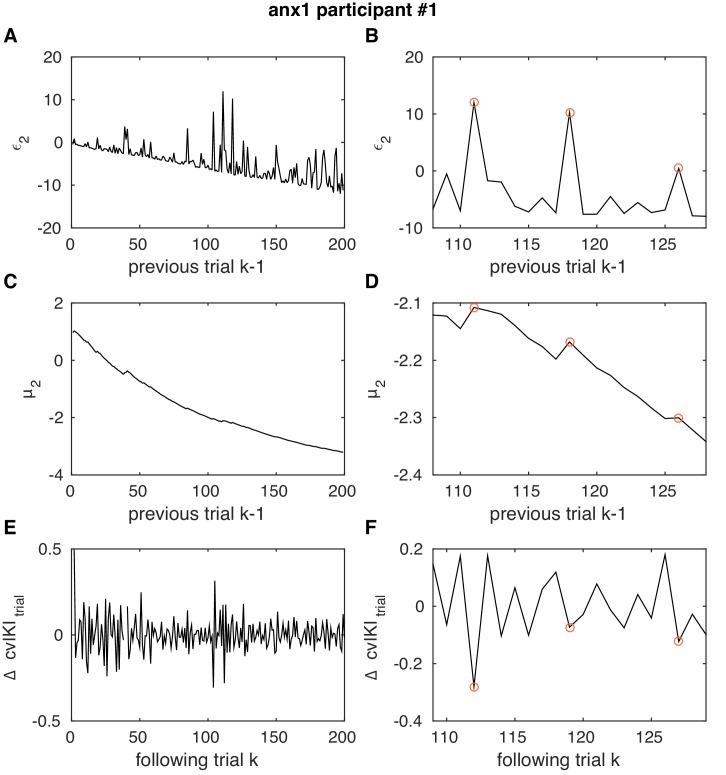
Example in one anx1 participant of the association between pwPEs relating to volatility and subsequent changes in performance. This figure illustrates the effect of negative ${\displaystyle {\beta }_2}$ coefficients in the response model in anx1 and anx2 participants, linking large ${\displaystyle {ϵ}_2}$ values to large changes in behavior on the next trial. Same as Figure 5—figure supplement 4 but in one participant from the anx1 group.

Figure 5—figure supplement 6. Grand-average trialwise residuals.

Grand-average trialwise residuals resulting from the difference between the observed responses and the responses predicted by the HGF. (A–C) The trialwise residuals in each control and experimental group are shown together as mean and SEM (shaded areas). The winning response model used as response variable the trial-by-trial change in ${\mathrm{cvIKI}}_{\mathrm{trial}}$, which is related to the temporal variability of IKI across keystroke positions in a trial. There were no systematic differences in the model fits across groups ($P>0.05$; between-group differences in the mean residual, after averaging across trials — cont: ${\displaystyle 0.0004[0.00095]}$; anx1: $-0.001[0.0013]$; anx2: $0.0003[0.0003]$). In the additional control experiment, we also found no significant differences between groups in the mean residual values (mean residual values per group: cont: $-0.0003[0.00047]$; anx3: ${\displaystyle -0.0023[0.0016]}$).