A novel kernel Wasserstein distance on Gaussian measures: an application of identifying dental artifacts in head and neck computed tomography

Abstract

The Wasserstein distance is a powerful metric based on the theory of optimal mass transport. It gives a natural measure of the distance between two distributions with a wide range of applications. In contrast to a number of the common divergences on distributions such as Kullback-Leibler or Jensen-Shannon, it is (weakly) continuous, and thus ideal for analyzing corrupted and noisy data. Until recently, however, no kernel methods for dealing with nonlinear data have been proposed via the Wasserstein distance. In this work, we develop a novel method to compute the L²-Wasserstein distance in reproducing kernel Hilbert spaces (RKHS) called kernel L²-Wasserstein distance, which is implemented using the kernel trick. The latter is a general method in machine learning employed to handle data in a nonlinear manner. We evaluate the proposed approach in identifying computed tomography (CT) slices with dental artifacts in head and neck cancer, performing unsupervised hierarchical clustering on the resulting Wasserstein distance matrix that is computed on imaging texture features extracted from each CT slice. We further compare the performance of kernel Wasserstein distance with alternatives including kernel Kullback-Leibler divergence we previously developed. Our experiments show that the kernel approach outperforms classical non-kernel approaches in identifying CT slices with artifacts.

1. Introduction

Optimal mass transport (OMT) theory is an old research area with its roots in civil engineering (Monge 1781) and economics (Kantorovich 1942) [1]. Recently there has been an ever increasing growth in OMT research both theoretically and practically, with impact on numerous fields including medical imaging analysis, statistical physics, machine learning, and genomics [2, 3, 4, 5]. The classical OMT problem formulated by Monge in 1781 concerns finding the optimal way via the minimization of a transportation cost required to move a pile of soil from one site to another [6, 7, 8, 9]. Let X and Y denote two probability spaces with measures μ and v, respectively, and let c(x, y) denote the transportation cost for moving one unit of mass from x ∈ X to y ∈ Y . Then the OMT problem seeks to find a (measurable) transport map T : X → Y that minimizes the total transportation cost ${\int }_X\mathbf{\text{C}}(x,T(x))\mu (dx)$. In 1942, Kantorovich proposed a relaxed formulation that transforms the Monge’s nonlinear problem to a linear programming problem [8]. Based on the Kantorovich’s formulation, the L^p- Wasserstein distance between μ and v on ${ℝ}^d$ is defined as:

$${\mathbf{\text{W}}}_p^p(\mu ,\nu )=\underset{\pi \in \Pi (\mu ,\nu )}{\text{inf}}{\int }_{{ℝ}^d\times {ℝ}^d}\Vert x-y{\Vert }^{p}d\pi (x,y),$$ (1)

where Π(μ, v) is the set of all joint probability measures π on X × Y whose marginals are μ and v. In particular, in the present study, we focus on L²- Wasserstein distance in which the squared Euclidean distance c(x, y) = ||x – y||² is the cost function [10].

Recently, a formulation to compute the Wasserstein distance between Gaussian measures in reproducing kernel Hilbert spaces (RKHS) was proposed by Zhang et al. [11]. In the present study, we propose a new alternative formulation to compute the Wasserstein distance in RKHS giving an explicit detailed proof, which is lacking in the Zhang et al. study. Both methods take O(n³) operations to compute the Wasserstein distance in RKHS due to the computation of square roots of a matrix [12] and nuclear norm in our approach and Zhang et al. study, respectively. Before introducing our proposed kernel Wasserstein distance, we first review some background on the kernel method.

The kernel computation in RKHS is based on the following idea. Suppose that we are given a data set of η samples in a native space, denoted by $\text{X=}\left[{\text{x}}_1,{\text{x}}_2,\cdots ,{\text{x}}_n\right]\in {ℝ}^d$. The input data can be mapped (transformed) into a higher dimensional feature space via a nonlinear mapping function ϕ [13, 14]. We let Φ := Φ_l×n [ϕ(x₁), (x₂), ⋯, ϕ(x_n)]denote the transformed data, where l is the number of features in the feature space (RKHS) with l > d. To avoid complex data handling in the feature space, and to avoid the explicit computation of the mapping funciton ϕ, typically one applies the kernel trick. More precisely, given any positive definite kernel function k, one can find an associated mapping function ϕ such that k(x, y) =< ϕ(x), ϕ(y) > with $\text{x},\text{y}\in {ℝ}^d$ [15, 16]. The resulting kernel Gram matrix K is defined as:

$$\mathbf{\text{K}}={\mathbf{\Phi }}^{\text{T}}\mathbf{\Phi },$$ (2)

where the ijth element, ϕ(x_i)^Tϕ(x_j), is computed using a kernel function k(x_i, x_j) =< ϕ(x_i), ϕ(x_j) >. Common choices of kernel functions are the polynomial and radial basis function (RBF) kernels [17]. In this study, the following RBF kernel will be employed:

$$k\left({\text{x}}_i,{\text{x}}_j\right)=\text{exp}\left(-\gamma {\Vert {\text{x}}_i-{\text{x}}_j\Vert }^2\right),$$ (3)

where γ > 0 controls the kernel width. We will fix γ = 1 in what follows. The mean and the covariance matrix in the feature space are given by:

$$\mu =\frac{1}{n}\sum _{i=1}^n\varphi \left({\text{x}}_i\right)={\mathbf{\Phi }}_{\mathbf{\text{s}}},\Sigma =\frac{1}{n}\sum _{i=1}^n\left(\varphi \left({\text{x}}_i\right)-\mu \right){\left(\varphi \left({\text{x}}_i\right)-\mu \right)}^{\text{T}}=\mathbf{\Phi }\mathbf{\text{J}}{\mathbf{\text{J}}}^{\text{T}}{\mathbf{\Phi }}^{\text{T}},$$ (4)

where ${\mathbf{\text{s}}}_{n\times 1}=\frac{1}{n}{\overrightarrow{1}}^{\text{T}}$, $\mathbf{\text{J}}=\frac{1}{\sqrt{n}}\left(I_n-\mathbf{\text{s}}\overrightarrow{1}\right)$, and $\overrightarrow{1}=[1,1,\cdots ,1]$. Then in Eq. (4), denoting ΦJ by W we have

$$\mathbf{\text{W}}=\mathbf{\Phi }\mathbf{\text{J}}=\frac{1}{\sqrt{n}}\left[\left(\varphi \left({\text{x}}_1\right)-\mu \right),\cdots ,\left(\varphi \left({\text{x}}_n\right)-\mu \right)\right].$$ (5)

Of note, these equations are used to compute the kernel Wasserstein distance as described in the following section.

2. Methods

In this section, we introduce the classical L²-Wasserstein distance between Gaussian measures and then propose a novel approach to compute L^2-Wasserstein distance in RKHS (denoted as kernel L²-Wasserstein distance). For comparison, we also provide a brief review of the Kullback-Leibler divergence in RKHS that we proposed in [18]. The code was implemented using MATLAB R2018b.

2.1. L²-Wasserstein Distance

For two Gaussian measures, v₁ = N₁(m₁, C₁) and v₂ = N₂ (m₂, C₂) on ${ℝ}^d$, the L²-Wasserstein distance between the two distributions may be computed as follows [19]:

$$W_2{\left({\nu }_1,{\nu }_2\right)}^2={\Vert {\mathbf{\text{m}}}_1-{\mathbf{\text{m}}}_2\Vert }^2+\text{tr}\left({\mathbf{\text{C}}}_1+{\mathbf{\text{C}}}_2-2{\left({\mathbf{\text{C}}}_1^{\frac{1}{2}}{\mathbf{\text{C}}}_2{\mathbf{\text{C}}}_1^{\frac{1}{2}}\right)}^{\frac{1}{2}}\right),$$ (6)

where tr is the trace. The term $\text{tr}\left({\mathbf{\text{C}}}_1+{\mathbf{\text{C}}}_2-2{\left({\mathbf{\text{C}}}_1^{\frac{1}{2}}{\mathbf{\text{C}}}_2{\mathbf{\text{C}}}_1^{\frac{1}{2}}\right)}^{\frac{1}{2}}\right)$ may be expressed as follows [20, 21, 22]:

$$\text{tr}\left({\mathbf{\text{C}}}_1+{\mathbf{\text{C}}}_2-2{\left({\mathbf{\text{C}}}_1^{\frac{1}{2}}{\mathbf{\text{C}}}_2{\mathbf{\text{C}}}_1^{\frac{1}{2}}\right)}^{\frac{1}{2}}\right)=\text{tr}\left({\mathbf{\text{C}}}_1+{\mathbf{\text{C}}}_2-2{\left({\mathbf{\text{C}}}_2{\mathbf{\text{C}}}_1\right)}^{\frac{1}{2}}\right).$$ (7)

For the convenience of the reader we include the explicit derivation of Eq. (7) in the Appendix.

2.2. L²-Wasserstein Distance in RKHS

We will now describe our formulation of the kernel L²-Wasserstein distance metric. Suppose that we are given two Gaussian measures, kv₁ and $k{\nu }_2\in {ℝ}^l$, in RKHS with mean μ_i and covariance matrix Σ_i, for i=1 and 2, and two sets of sample data in the native space, X = [x₁, x₂, ⋯, x_n] and $\mathbf{\text{Y}}=\left[{\text{y}}_1,{\text{y}}_2,\cdots ,{\text{y}}_m\right]\in {ℝ}^d$ associated with kv₁ and kv₂, respectively. The assumption that the data in RKHS follow a Gaussian distribution is based on the fact that data transformed by nonlinear kernels including RBF are more likely to be Gaussian, as justified by Huang et al. [23]. Then, as in Eq. (6), the L²-Wasserstein distance between the two distributions is given by:

$$W_2{\left(k{\nu }_1,k{\nu }_2\right)}^2={\Vert {\mu }_1-{\mu }_2\Vert }^2+\text{tr}\left({\Sigma }_1+{\Sigma }_2-2{\left({\Sigma }_1^{\frac{1}{2}}{\Sigma }_2{\Sigma }_1^{\frac{1}{2}}\right)}^{\frac{1}{2}}\right),$$ (8)

where the definitions of μ_i and Σ_i are shown in Eq. (4). As previously mentioned, $\text{tr}{\left({\Sigma }_1^{\frac{1}{2}}{\Sigma }_2{\Sigma }_1^{\frac{1}{2}}\right)}^{\frac{1}{2}}=\text{tr}{\left({\Sigma }_2{\Sigma }_1\right)}^{\frac{1}{2}}$. In Eq. (8), the first term ||μ₁ − μ₂||² (the squared maximum mean discrepancy) can be obtained as follows [24]:

$${\Vert {\mu }_1-{\mu }_2\Vert }^2={\Vert {\mu }_1\Vert }^2-2{\mu }_1^{\text{T}}{\mu }_2+{\Vert {\mu }_2\Vert }^2.$$ (9)

Via a simple computation, Eq. (9) may be expressed with kernel functions as follows:

$${\Vert {\mu }_1-{\mu }_2\Vert }^2=\frac{1}{n^2}\sum _{i=1}^n\sum _{j=1}^{n}k\left({\text{x}}_i,{\text{x}}_j\right)-\frac{2}{nm}\sum _{i=1}^n\sum _{j=1}^{m}k\left({\text{x}}_i,{\text{y}}_j\right)+\frac{1}{m^2}\sum _{i=1}^m\sum _{j=1}^{m}k\left({\text{y}}_i,{\text{y}}_j\right).$$ (10)

Now we simplify the last term in Eq. (8) by using Eq. (4) :

$$\text{tr}\left({\Sigma }_1+{\Sigma }_2-2{\left({\Sigma }_2{\Sigma }_1\right)}^{\frac{1}{2}}\right)=\text{tr}\left({\mathbf{\text{J}}}_1{\mathbf{\text{J}}}_1^{\text{T}}{\mathbf{\text{K}}}_{11}\right)+\text{tr}\left({\mathbf{\text{J}}}_2{\mathbf{\text{J}}}_2^{\text{T}}{\mathbf{\text{K}}}_{22}\right)-2\text{tr}{\left({\mathbf{\Phi }}_2\mathbf{\text{R}}{\mathbf{\Phi }}_1^{\text{T}}\right)}^{\frac{1}{2}},$$ (11)

where $\mathbf{\text{R}}={\mathbf{\text{J}}}_2{\mathbf{\text{J}}}_2^{\text{T}}{\mathbf{\text{K}}}_{21}{\mathbf{\text{J}}}_1{\mathbf{\text{J}}}_1^{\text{T}}$ and ${\mathbf{\text{K}}}_{ij}={\mathbf{\Phi }}_i^{\text{T}}{\mathbf{\Phi }}_j$ . We give the full proof of Eq. (11) in the Appendix. Note that Σ₁ and Σ₂ are symmetric positive semidefinite. Therefore, ${\Sigma }_2{\Sigma }_1={\mathbf{\Phi }}_2\mathbf{\text{R}}{\mathbf{\Phi }}_1^{\text{T}}$ is diagonalizable and has nonnegative eigenvalues. Suppose that the eigenvector and eigenvalue matrices of ${\mathbf{\Phi }}_2\mathbf{\text{R}}{\mathbf{\Phi }}_1^{\text{T}}$ are $\widetilde{\mathbf{\text{P}}}$ and $\tilde{\Lambda }$:

$${\mathbf{\Phi }}_2\mathbf{\text{R}}{\mathbf{\Phi }}_1^{\text{T}}\widetilde{\mathbf{\text{P}}}=\widetilde{\mathbf{\text{P}}}\tilde{\Lambda }.$$ (12)

By multiplying both sides by ${\mathbf{\Phi }}_1^{\text{T}}$, we have ${\mathbf{\Phi }}_1^{\text{T}}{\mathbf{\Phi }}_2\mathbf{\text{R}}{\mathbf{\Phi }}_1^{\text{T}}\widetilde{\mathbf{\text{P}}}={\mathbf{\Phi }}_1^{\text{T}}\widetilde{\mathbf{\text{P}}}\tilde{\Lambda }$. That is, the eigenvalue matrix of ${\mathbf{\Phi }}_1^{\text{T}}{\mathbf{\Phi }}_2\mathbf{\text{R}}$ is the same as that of ${\mathbf{\Phi }}_2\mathbf{\text{R}}{\mathbf{\Phi }}_1^{\text{T}}$ with $\tilde{\Lambda }$. Therefore, the following equations hold:

$$\text{tr}{\left({\mathbf{\Phi }}_2\mathbf{\text{R}}{\mathbf{\Phi }}_1^{\text{T}}\right)}^{\frac{1}{2}}=\text{tr}{\left({\mathbf{\Phi }}_1^{\text{T}}{\mathbf{\Phi }}_2\mathbf{\text{R}}\right)}^{\frac{1}{2}}=\text{tr}{\left({\mathbf{\text{K}}}_{12}\mathbf{\text{R}}\right)}^{\frac{1}{2}}=\text{tr}{\left({\mathbf{\text{K}}}_{12}{\mathbf{\text{J}}}_2{\mathbf{\text{J}}}_2^{\text{T}}{\mathbf{\text{K}}}_{21}{\mathbf{\text{J}}}_1{\mathbf{\text{J}}}_1^{\text{T}}\right)}^{\frac{1}{2}}.$$ (13)

Finally, using Eq. (10) and Eq. (13), the kernel L²-Wasserstein distance may be expressed as:

$$\begin{gathered} W_2{\left(k{\nu }_1,k{\nu }_2\right)}^2={\Vert {\mu }_1-{\mu }_2\Vert }^2+\text{tr}\left({\Sigma }_1+{\Sigma }_2-2{\left({\Sigma }_1^{\frac{1}{2}}{\Sigma }_2{\Sigma }_1^{\frac{1}{2}}\right)}^{\frac{1}{2}}\right) \\ =\frac{1}{n^2}\sum _{i=1}^n\sum _{j=1}^{n}k\left({\text{x}}_i,{\text{x}}_j\right)-\frac{2}{nm}\sum _{i=1}^n\sum _{j=1}^{m}k\left({\text{x}}_i,{\text{y}}_j\right)+\frac{1}{m^2}\sum _{i=1}^m\sum _{j=1}^{m}k\left({\text{y}}_i,{\text{y}}_j\right) \\ +\text{tr}\left({\mathbf{\text{J}}}_1{\mathbf{\text{J}}}_{\text{1}}^{\text{T}}{\mathbf{\text{K}}}_{11}\right)+\text{tr}\left({\mathbf{\text{J}}}_2{\mathbf{\text{J}}}_2^{\text{T}}{\mathbf{\text{K}}}_{22}\right)-2\text{tr}{\left({\mathbf{\text{K}}}_{12}{\mathbf{\text{J}}}_2{\mathbf{\text{J}}}_2^{\text{T}}{\mathbf{\text{K}}}_{21}{\mathbf{\text{J}}}_1{\mathbf{\text{J}}}_1^{\text{T}}\right)}^{\frac{1}{2}}. \end{gathered}$$ (14)

When Σ₁ is the same as Σ₂, we have

$$W_2{\left(k{\nu }_1,k{\nu }_2\right)}^2=\frac{1}{n^2}\sum _{i=1}^n\sum _{j=1}^{n}k\left({\text{x}}_i,{\text{x}}_j\right)-\frac{2}{nm}\sum _{i=1}^n\sum _{j=1}^{m}k\left({\text{x}}_i,{\text{y}}_j\right)+\frac{1}{m^2}\sum _{i=1}^m\sum _{j=1}^{m}k\left({\text{y}}_i,{\text{y}}_j\right).$$

2.3. Kullback-Leibler Divergence in RKHS

Kullback-Leibler (KL) divergence is another type of method to compare two probability distributions [25]. It is not a distance measure due to its asymmetric nature. Let P and Q be two continuous probability distributions with the corresponding probability densities p(x) and q(x), respectively. Then the KL divergence or relative entropy of P and Q over the same variable x is defined as:

$$D_{\text{KL}}(P\Vert Q)={\int }_{-\infty }^{\infty }p(x)\text{\hspace{0.17em}log}\frac{p(x)}{q(x)}dx,$$ (15)

where D_KL(P||Q) equals zero if and only if P = Q. Given two Gaussian measures in RKHS, N₁(μ₁, Σ₁) and N₂(μ₂, Σ₂) with both $\in {ℝ}^l$, the KL divergence may be computed to be:

$$D_{\text{KL}}\left(N_1\Vert N_2\right)=\frac{1}{2}\left\{{\left({\mu }_1-{\mu }_2\right)}^{\text{T}}{\Sigma }_2^{-1}\left({\mu }_1-{\mu }_2\right)+\text{log}\frac{|{\Sigma }_2|}{|{\Sigma }_1|}+\text{tr}\left[{\Sigma }_1{\Sigma }_2^{-1}\right]-l\right\},$$ (16)

where |Σ_i| is the determinant of covariance matrix Σ_i. Note that l is the number of features in RKHS and indeed this is unknown. Importantly, this variable is canceled out when Eq. (16) is completely solved, which will be explained later. In a special case, when $\Sigma ={\Sigma }_1={\Sigma }_2,D_{\text{KL}}\left(N_1\Vert N_2\right)=\frac{1}{2}\left\{{\left({\mu }_1-{\mu }_2\right)}^{\text{T}}{\Sigma }^{-1}\left({\mu }_1-{\mu }_2\right)\right\}$.

2.3.1. Singularity Problem

In many real-world problems, the number of samples is considerably smaller than the number of features, leading to the covariance matrix being singular, and therefore non-invertible. Typically, one deals with data in a higher dimensional space as in this study. To avoid the singularity problem, several methods have been proposed [26, 27]. In this work, we employ a straightforward scheme by adding a positive value to the diagonal elements of the covariance matrix [28]. Therefore, the modified covariance matrix is of full rank and invertible. Set

$$\mathbf{\text{H}}=\Sigma +\rho {\mathbf{\text{I}}}_l=\mathbf{\Phi }\mathbf{\text{J}}{\mathbf{\text{J}}}^{\text{T}}{\mathbf{\Phi }}^{\text{T}}+\rho {\mathbf{\text{I}}}_l=\mathbf{\text{W}}{\mathbf{\text{W}}}^{\text{T}}+\rho {\mathbf{\text{I}}}_l=\mathbf{\Phi }\mathbf{\text{S}}{\mathbf{\Phi }}^{\text{T}}+\rho {\mathbf{\text{I}}}_l,$$ (17)

where W = ΦJ as in Eq. (5), S = JJ^T, l is the number of features, and I_l is an l × l identity matrix. In this study, ρ = 0.1 is used.

In the next computation, we will employ the Woodbury formula [29], which we now review. Let A be a square r × r invertible matrix, and let U and V be matrices of size r × k with k ≤r. Assume that the k × k matrix Σ = I_k + β+V^TA⁻¹U is invertible, where β is an arbitrary scalar. Then the Woodbury formula states that

$${\left(\mathbf{\text{A}}+\beta \mathbf{\text{U}}{\mathbf{\text{V}}}^{\text{T}}\right)}^{-1}={\mathbf{\text{A}}}^{-1}-\beta {\mathbf{\text{A}}}^{-1}\mathbf{\text{U}}{\Sigma }^{-1}{\mathbf{\text{V}}}^{\text{T}}{\mathbf{\text{A}}}^{-1}.$$

Accordingly, utilizing this formula, we can compute the inverse of H:

$$\begin{gathered} {\mathbf{\text{H}}}^{-1}={\left(\rho {\mathbf{\text{I}}}_l+\mathbf{\Phi }\mathbf{\text{J}}{\mathbf{\text{J}}}^{\text{T}}{\mathbf{\Phi }}^{\text{T}}\right)}^{-1} \\ ={\left(\rho {\mathbf{\text{I}}}_l+\mathbf{\text{W}}{\mathbf{\text{W}}}^{\text{T}}\right)}^{-1}⊲\text{apply }\mathit{\text{Woodbury }}\mathit{\text{formula\hspace{0.17em}}} \\ ={\rho }^{-1}\left({\mathbf{\text{I}}}_l-\mathbf{\Phi }\mathbf{\text{B}}{\mathbf{\Phi }}^{\text{T}}\right), \end{gathered}$$ (18)

where $\mathbf{\text{B}}=\mathbf{\text{J}}{\mathbf{\text{M}}}^{-1}{\mathbf{\text{J}}}^{\text{T}}$, $\mathbf{\text{M}}=\rho {\mathbf{\text{I}}}_n+{\mathbf{\text{W}}}^{\text{T}}\mathbf{\text{W}}=\rho {\mathbf{\text{I}}}_n+{\mathbf{\text{J}}}^{\text{T}}{\mathbf{\Phi }}^{\text{T}}\mathbf{\Phi }\mathbf{\text{J}}=\rho {\mathbf{\text{I}}}_n+{\mathbf{\text{J}}}^{\text{T}}K\mathbf{\text{J}}$, and n is the number of samples. In H⁻¹, some mapping functions are still left. These will be replaced with kernel functions when kernel KL divergence is completely solved. See the Appendix for all the details regarding the derivation of Eq. (18).

2.3.2. Calculation of Kernel KL Divergence

In the Experiments section below, we will compare Wasserstein distance and KL divergence based kernel methods. Accordingly, we sketch the necessary theory for the kernel KL divergence approach.

Suppose that we are given two Gaussian measures in RKHS, N₁(μ₁, Σ₁) and $N_2\left({\mu }_2,{\Sigma }_2\right)\in {ℝ}^l$, consisting of n and m samples, respectively. Assume that Σ₁ and Σ₂ are singular in the higher dimensional space. Let H₁ and H₂ denote the approximate covariance matrices for the two distributions as in Eq. (17). Then, the kernel KL divergence is expressed as follows:

$$2D_{\text{KL}}\left(N_1\Vert N_2\right)={\left({\mu }_1-{\mu }_2\right)}^{\text{T}}{\mathbf{\text{H}}}_2^{-1}\left({\mu }_1-{\mu }_2\right)+\text{log}\frac{|{\mathbf{\text{H}}}_2|}{|{\mathbf{\text{H}}}_1|}+\text{tr}\left[{\mathbf{\text{H}}}_1{\mathbf{\text{H}}}_2^{-1}\right]-l.$$ (19)

We now solve each term separately: (1) ${\left({\mu }_1-{\mu }_2\right)}^{\text{T}}{\mathbf{\text{H}}}_2^{-1}\left({\mu }_1-{\mu }_2\right)$, (2) $\text{log}\frac{|{\mathbf{\text{H}}}_2|}{|{\mathbf{\text{H}}}_1|}$, and (3) $\text{tr}\left[{\mathbf{\text{H}}}_1{\mathbf{\text{H}}}_2^{-1}\right]$. The first term consists of four sub-terms:

$${\left({\mu }_1-{\mu }_2\right)}^{\text{T}}{\mathbf{\text{H}}}_2^{-1}\left({\mu }_1-{\mu }_2\right)={\mu }_1^{\text{T}}{\mathbf{\text{H}}}_2^{-1}{\mu }_1+{\mu }_2^{\text{T}}{\mathbf{\text{H}}}_2^{-1}{\mu }_2-{\mu }_1^{\text{T}}{\mathbf{\text{H}}}_2^{-1}{\mu }_2-{\mu }_2^{\text{T}}{\mathbf{\text{H}}}_2^{-1}{\mu }_1$$ (20)

Substituting Eq. (4) and Eq. (18) into each sub-term ${\mu }_i^{\text{T}}{\mathbf{\text{H}}}_j^{-1}{\mu }_k$, we have

$$\begin{gathered} {\mu }_i^{\text{T}}{\mathbf{\text{H}}}_j^{-1}{\mu }_k={\mathbf{\text{s}}}_i^{\text{T}}{\mathbf{\Phi }}_i^{\text{T}}{\rho }^{-1}\left(I_l-{\mathbf{\Phi }}_j{\mathbf{\text{B}}}_j{\mathbf{\Phi }}_j^{\text{T}}\right){\mathbf{\Phi }}_k{\mathbf{\text{s}}}_k \\ ={\rho }^{-1}\left({\mathbf{\text{s}}}_i^{\text{T}}{\mathbf{\text{K}}}_{ik}{\mathbf{\text{s}}}_k-{\mathbf{\text{s}}}_i^{\text{T}}{\mathbf{\text{K}}}_{ij}{\mathbf{\text{B}}}_j{\mathbf{\text{K}}}_{jk}{\mathbf{\text{s}}}_k\right) \\ ={\rho }^{-1}{\theta }_{ijk}, \end{gathered}$$ (21)

where ${\theta }_{ijk}={\mathbf{\text{s}}}_i^{\text{T}}{\mathbf{\text{K}}}_{ik}{\mathbf{\text{s}}}_k-{\mathbf{\text{s}}}_i^{\text{T}}{\mathbf{\text{K}}}_{ij}{\mathbf{\text{B}}}_j{\mathbf{\text{K}}}_{jk}{\mathbf{\text{s}}}_k$. As a result, all the mapping functions in the first term can be replaced with kernel functions. For the second term, we need to compute the determinant of H. To accomplish this, we use a simple trick by computing the determinant of H⁻¹ instead of H.

$$\begin{gathered} |{\mathbf{\text{H}}}_1^{-1}|=|{\rho }^{-1}\left({\mathbf{\text{I}}}_l-{\mathbf{\Phi }}_1{\mathbf{\text{B}}}_1{\mathbf{\Phi }}_1^{\text{T}}\right)| \\ ={\rho }^{-l}|{\mathbf{\text{I}}}_l-{\mathbf{\text{Q}}}_1{\mathbf{\Phi }}_1^{\text{T}}| \\ ={\rho }^{-l}|{\mathbf{\text{I}}}_n-{\mathbf{\text{K}}}_{11}{\mathbf{\text{B}}}_1|, \end{gathered}$$ (22)

where Q₁ = Φ₁B₁. See the Appendix for the complete derivation of Eq. (22). Now we compute |H₁| as follows:

$$|{\mathbf{\text{H}}}_1|=\frac{1}{|{\mathbf{\text{H}}}_1-1|}=\frac{{\rho }^l}{|{\mathbf{\text{I}}}_n-{\mathbf{\text{K}}}_{11}{\mathbf{\text{B}}}_1|}.$$ (23)

By taking logarithm of |H₁|, we have

$$\text{log}|{\mathbf{\text{H}}}_1|=\text{log}\frac{{\rho }^l}{|{\mathbf{\text{I}}}_n-{\mathbf{\text{K}}}_{11}{\mathbf{\text{B}}}_1|}=l\text{log}\rho -\text{log}|{\mathbf{\text{I}}}_n-{\mathbf{\text{K}}}_{11}{\mathbf{\text{B}}}_1|.$$ (24)

Therefore, we have the second term composed of kernel functions:

$$\text{log}\frac{|{\mathbf{\text{H}}}_2|}{|{\mathbf{\text{H}}}_1|}=\text{log}|{\mathbf{\text{H}}}_2|-\text{log}|{\mathbf{\text{H}}}_1|=\text{log}|{\mathbf{\text{I}}}_n-{\mathbf{\text{K}}}_{11}{\mathbf{\text{B}}}_1|-\text{log}|{\mathbf{\text{I}}}_m-{\mathbf{\text{K}}}_{22}{\mathbf{\text{B}}}_2|.$$ (25)

The third term can be replaced with kernel functions using properties of trace (see the Appendix for all the details of the derivation):

$$\text{tr}\left[{\mathbf{\text{H}}}_1{\mathbf{\text{H}}}_2^{-1}\right]={\rho }^{-1}\text{tr}\left[{\mathbf{\text{S}}}_1{\mathbf{\text{K}}}_{11}\right]-{\rho }^{-1}\text{tr}\left[{\mathbf{\text{S}}}_1{\mathbf{\text{K}}}_{12}{\mathbf{\text{B}}}_2{\mathbf{\text{K}}}_{21}\right]+l-\text{tr}\left[{\mathbf{\text{B}}}_2{\mathbf{\text{K}}}_{22}\right].$$ (26)

Consequently, we have solved kernel KL divergence by replacing all mapping functions with kernel functions and it is expressed as follows:

$$\begin{gathered} 2D_{\text{KL}}\left(N_1\Vert N_2\right)={\left({\mu }_1-{\mu }_2\right)}^{\text{T}}{\mathbf{\text{H}}}_2^{-1}\left({\mu }_1-{\mu }_2\right)+\text{log}\frac{|{\mathbf{\text{H}}}_2|}{|{\mathbf{\text{H}}}_1|}+\text{tr}\left[{\mathbf{\text{H}}}_1{\mathbf{\text{H}}}_2^{-1}\right]-l \\ ={\rho }^{-1}\left({\theta }_{121}+{\theta }_{222}-{\theta }_{122}-{\theta }_{221}\right)+\text{log}|{\mathbf{\text{I}}}_n-{\mathbf{\text{K}}}_{11}{\mathbf{\text{B}}}_1|-\text{\hspace{0.17em}log}|{\mathbf{\text{I}}}_m-{\mathbf{\text{K}}}_{22}{\mathbf{\text{B}}}_2|+{\rho }^{-1}\text{tr}\left[{\mathbf{\text{S}}}_1{\mathbf{\text{K}}}_{11}\right]-{\rho }^{-1}\text{tr}\left[{\mathbf{\text{S}}}_1{\mathbf{\text{K}}}_{12}{\mathbf{\text{B}}}_2{\mathbf{\text{K}}}_{21}\right]-\text{tr}\left[{\mathbf{\text{B}}}_2{\mathbf{\text{K}}}_{22}\right]. \end{gathered}$$ (27)

Note that the l is canceled out. Moreover, since D_KL(P||Q) ≠ D_KL(Q||P), in this study an average value of two KL measures is used: $J_{\text{KL}}(P\Vert Q)=\frac{1}{2}\left\{D_{\text{KL}}(P\Vert Q)+D_{\text{KL}}(Q\Vert P)\right\}$ [30].

3. Experiments

3.1. Data

We investigated the utility of kernel L²-Wasserstein distance to identify slices with dental artifacts in computed tomography (CT) scans in head and neck cancer. Serious image degradation caused by metallic fillings or crowns in teeth is a common problem in CT images. We analyzed 1164 axial slices from 44 CT scans that were collected from 44 patients with head and cancer who were treated in our institution. This retrospective study was approved by the institutional review board and informed consent was obtained from all patients. Before the analysis, each CT slice was labeled as noisy or clean based on the presence of dental artifacts by a medical imaging expert, resulting in 276 noisy and 888 clean slices. Figure 1 shows representative noisy and clean CT slices from two different scans.

Figure 1:

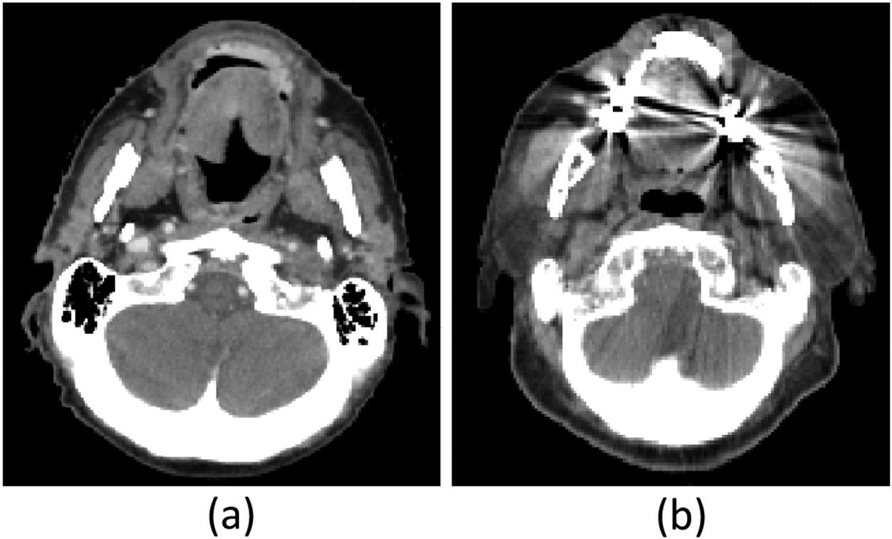
Representative clean (a) and noisy (b) slices.

3.2. Texture Features

Intensity thresholding (at the 5th percentile) was performed to exclude air voxels on each CT slice. The Computational Environment for Radiological Research (CERR) radiomics toolbox was then used to calculate the gray-level co-occurrence matrix (GLCM) from the remaining voxels using 64 gray levels and with a neighborhood of 8 voxels across all 4 directions in 2D [31, 32]. A total of 25 scalar features were then extracted from the GLCM (listed in Table 1). For further information on the GLCM features used, see https://github.com/cerr/CERR/wiki/Radiomics. Each feature was nomalized between 0 and 1 for further analysis.

Table 1:

GLCM-based 25 texture features used in this study.

No	Features	No	Features
1	Auto-correlation	14	Inverse Difference Moment
2	Joint Average	15	First Informal Correlation
3	Cluster Prominence	16	Second Informal Correlation
4	Cluster Shade	17	Inverse Difference Moment Normalized
5	Cluster Tendency	18	Inverse Difference Normalized
6	Contrast	19	Inverse Variance
7	Correlation	20	Sum Average
8	Difference Entropy	21	Sum Entropy
9	Dissimilarity	22	Sum Variance
10	Difference Variance	23	Haralick Correlation
11	Joint Energy	24	Joint Maximum
12	Joint Entropy	25	Joint Variance
13	Inverse Difference

3.3. Experimental Results

For 1164 CT slices, we computed kernel L²-Wasserstein distance between each pair of slices on 25 GLCM-based texture features. After that, we conducted unsupervised hierarchical clustering using the resulting distance matrix. Figure 2a shows a heatmap of the symmetric distance matrix for each pair of slices and Figure 2b presents the hierarchical clustering result. We identified two clusters: Cluster 1 with blue lines and Cluster 2 with red lines, consisting of 666 and 498 slices, respectively. In Figure 2b, the bar under the hierarchical graph indicates the actual labels with blue for clean slices and red for noisy slices. As a result, Cluster 1 has 658 clean and 8 noisy slices whereas Cluster 2 has 230 clean and 268 noisy slices (table in Figure 2b). That is, Cluster 1 and 2 were significantly enriched for clean and noisy slices, respectively, with a Chi-square test p-value < 0.0001. Prediction rates were 97.10% and 74.10% for noisy and clean slices, respectively, and overall prediction rate was 79.6%. In Figure 2a, the order of slices is the same as that shown in Figure 2b and the two clusters were divided by the black dot lines; the left bottom block represents Cluster 1 and the right top block for Cluster 2. The areas with blue color indicate close distance between slices whereas the areas with red color indicate far distance. Not surprisingly, the blue areas are mostly shown in the two blocks that represent the distances within each cluster. On the other hand, other two blocks (in the left top and right bottom) mostly have red areas, implying far distance between the two clusters (between noisy and clean slices).

Figure 2:

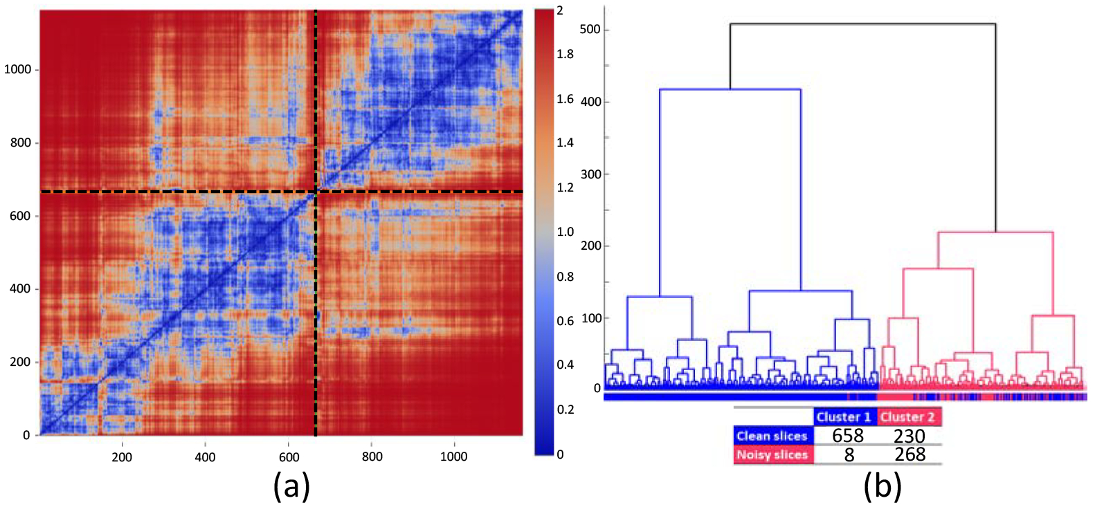
Results for kernel Wasserstein distance: (a) heatmap for the resulting distance matrix and (b) hierarchical clustering result conducted using the distance matrix.

We compared performance of kernel L²-Wasserstein distance with other methods, including Wasserstein distance and KL and kernel KL divergence, using Chi-square statistic. Note that for KL and kernel KL divergence we computed the average value of two KL measures, i.e., J_KL(P||Q). We repeated the analysis process noted above for alternative methods. Of note, kernel methods (kernel Wasserstein distance and kernel KL divergence) had the same accuracy with a Chi-square statistic of 436 (Figure 3). By contrast, non-kernel methods (Wasserstein distance and KL divergence) had substantially lower Chi-square statistics with 21 and 91, respectively, showing the superiority of kernel methods in this application.

Figure 3:

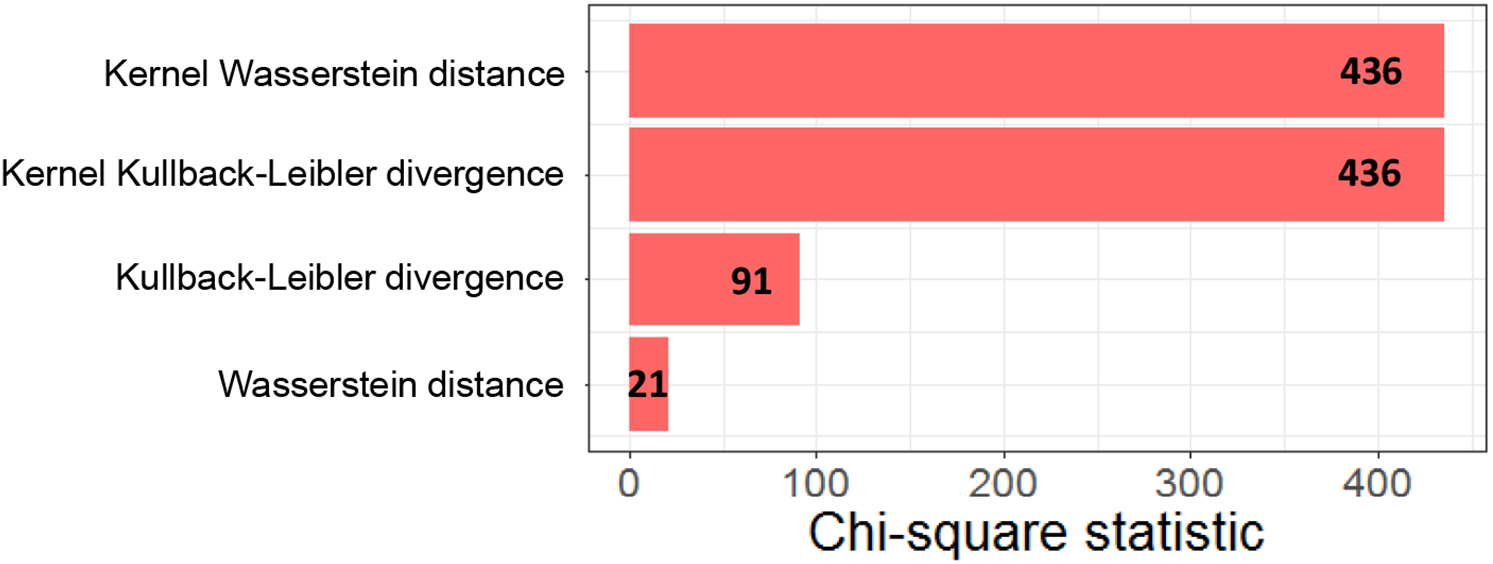
Chi-square statistics for four methods: Wasserstein distance, kernel Wasserstein distance, Kullback-Leibler divergence, and kernel Kullback-Leibler divergence.

The basic idea of kernel mean embedding is to map distributions into RKHS by representing each distribution as a mean function [33]. As a baseline test, the Maximum Mean Discrepancy (MMD) that indicates the RKHS-distance between two mapped measures on the space of probability measures was computed. Its Chi-square statistic was 410, which was lower than that of kernel methods.

We examined the performance difference between kernel Wasserstein distance and Wasserstein distance shown in Figure 3 using Pearson correlation tests. For the clustering results of kernel Wasserstein distance shown in Figure 2b, Pearson correlation coefficients between kernel Wasserstein distance and Wasserstein distance were 0.61, 0.62, and 0.47 in Cluster 1 (Figure 4a), Cluster 2 (Figure 4b), and between two clusters (Figure 4c), respectively. In addition, the correlation between the two methods in Cluster 2 that was enriched for noisy slices showed a relatively more linear pattern. This suggests that the superior performance of kernel Wasserstein distance is likely due to better prediction in Cluster 1 than the Wasserstein distance.

Figure 4:

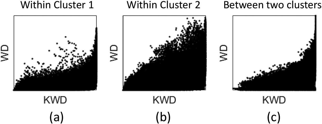
Scatter plots for the correlation between kernel Wasserstein distance and Wasserstein distance in (a) Cluster 1, (b) Cluster 2, and (c) between two clusters. KWD: kernel Wasserstein distance and WD: Wasserstein distance.

3.4. Computation Time

The computation time was compared for four different approaches. We used a PC with Intel Xeon CPU E5–2620 v3 @ 2.40GHz and 32GB RAM. Averaged running time after 10 runs was 13, 19, 8, and 19 seconds for kernel Wasserstein distance, kernel Kullback-Leibler divergence, Wasserstein distance, and Kullback-Leibler divergence, respectively. The computation time of kernel Wasserstein distance was faster than the kernel Kullback-Leibler divergence.

4. Discussion

The Wasserstein distance is a very versatile tool with a wide range of applications. Although extensively used, a method of computing this metric in RKHS has been lacking. In this paper, we proposed a new computational method to solve L²-Wasserstein distance in RKHS with a detailed derivation. Although the current study and the work of Zhang et al. [11] treat the same problem, the final solutions to compute kernel Wasserstein distance are not the same. More importantly, we described the procedure to obtain the final equation clearly and simply whereas in the Zhang et al. paper, there is no detailed process or proof to reach the equation. This is a significant contribution in the current study.

We applied the proposed technique to a medical imaging problem in which CT scans are often degraded by artifacts arising from high-density materials. Our unsupervised method consisting of kernel L²-Wasserstein distance and hierarchical clustering showed a good level of performance in identifying noisy CT slices, outperforming conventional Wasserstein distance. Notably, kernel Kullback-Leibler divergence also obtained comparable performance. This implies the nonlinearity of data and thus nonlinear analysis using kernel methods would be more likely to be essential.

Welch et al. (2020) developed a convolutional neural network model to classify dental artifact statuses on head and neck CT images which can automate image quality assurance tasks required for unbiased image analysis research [34]. Wei et al. (2019) developed a random forest model for CT artifacts detection and showed such dental artifacts in head and neck CT images have a negative impact on the performance in radiomics research [35]. These studies used supervised learning methods. In contrast, our approach is a fully unsupervised method and thus it is not feasible to directly compare the performance of our approach with those methods. We plan to develop a new supervised OMT method.

The clustering results showed that noisy slices are better clustered than clean slices. To demonstrate the application of kernel Wasserstein distance, we used only GLCM texture features that are the most frequently utilized texture features. Recently, several new types of texture features have been developed including the gray level run length matrix (GLRLM), the gray level size zone matrix (GLSZM), the neighborhood gray tone difference matrix (NGTDM), and the neighboring gray level dependence matrix (NGLDM), which can detect different patterns of textures on images [31]. Adding such texture features in our analysis is likely to improve a specificity of clustering clean slices, which is a goal of our future work.

A limitation of the current study is that there is no adequate experiment to show the benefit of Wasserstein distance in RKHS. The goal of this study was focusing on proposing a novel computational method and demonstrating the feasibility of the approach. That is, this study was intended to be a proof of concept of using the proposed computation method prior to actively applying it to more datasets. Future work will focus on further applications of kernel L²-Wasserstein distance in imaging and biological data analysis.

Highlights.

• A novel method to compute the L²-Wasserstein distance in reproducing kernel Hilbert spaces was proposed.

• The resultant kernel Wasserstein distance matrix was integrated with a conventional hierarchical clustering method for grouping samples.

• The proposed approach was used to identify computed tomography slices with dental artifacts in head and neck cancer using radiomics.

Biography

Jung Hun Oh received the PhD degree in Computer Science from the University of Texas, Arlington in 2008. He is currently an Assistant Attending Computer Scientist with the Department of Medical Physics, Memorial Sloan Kettering Cancer Center. His current research interests include outcomes modeling, radiomics, and radiogenomics in cancer using machine learning and bioinformatics techniques.

Maryam Pouryahya received the PhD degree in Applied Mathematics & Statistics, Stony Brook University in 2018. She is a postdoctoral fellow in the Department of Medical Physics, Memorial Sloan Kettering Cancer Center. Her research focuses on multi-omics data integration and drug response prediction based on optimal mass transport theory.

Aditi Iyer received the MS degree in Electrical and Computer Engineering from Purdue University in 2015. She is a key contributor to the development of the Computational Environment for Radiological Research (CERR), an open-source software tool for image and dosimetry analysis. Her research interests include developing algorithms for medical image analysis, particularly image segmentation, using machine learning methods.

Aditya P. Apte received the PhD degree in Mechanical Engineering from the University of Texas, Arlington in 2009. He is currently an Assistant Attending Physicist with the Department of Medical Physics, Memorial Sloan Kettering Cancer Center. He is the lead architect and programmer for the open source informatics tool, the Computational Environment for Radiological Research (CERR). His research interests include medical image analysis and radiomics.

Joseph O. Deasy is the Chair of the Department of Medical Physics and Chief of the Service for Predictive Informatics (SPI) at Memorial Sloan Kettering Cancer Center. He created the SPI in 2011 with a mission of conducting image-based/big data analyses, and advancing new clinical decision support tools, e.g., imagebased radiation oncology, radiomics, imaging genomics, tumor response, toxicity prediction, and genomebased predictive models. He has over 20 years of experience in data science and informatics, including creating the CERR software platform.

Allen Tannenbaum is a Distinguished Professor of Computer Science and Applied Mathematics & Statistics at Stony Brook University as well as Affiliate Attending Computer Scientist at Memorial Sloan Kettering Cancer Center. His research interests are in systems and control, network theory, computer vision, systems biology, and medical image processing.

Appendix

Here, we prove equations used in the paper.

Proof of Eq. (7):

$$\text{tr}\left({\mathbf{\text{C}}}_1+{\mathbf{\text{C}}}_2-2{\left({\mathbf{\text{C}}}_1^{\frac{1}{2}}{\mathbf{\text{C}}}_2{\mathbf{\text{C}}}_1^{\frac{1}{2}}\right)}^{\frac{1}{2}}\right)=\text{tr}\left({\mathbf{\text{C}}}_1+{\mathbf{\text{C}}}_2-2{\left({\mathbf{\text{C}}}_2{\mathbf{\text{C}}}_1\right)}^{\frac{1}{2}}\right)$$

For convenience, we sketch the proof of this fact. Indeed, by the linearity of the trace, $\text{tr}\left({\mathbf{\text{C}}}_1+{\mathbf{\text{C}}}_2-2{\left({\mathbf{\text{C}}}_2{\mathbf{\text{C}}}_1\right)}^{\frac{1}{2}}\right)=\text{tr}\left({\mathbf{\text{C}}}_1\right)+\text{tr}\left({\mathbf{\text{C}}}_2\right)-2\text{tr}{\left({\mathbf{\text{C}}}_2{\mathbf{\text{C}}}_1\right)}^{\frac{1}{2}}$. herefore, we need to prove that $\text{tr}{\left({\mathbf{\text{C}}}_2{\mathbf{\text{C}}}_1\right)}^{\frac{1}{2}}=\text{tr}{\left({\mathbf{\text{C}}}_1^{\frac{1}{2}}{\mathbf{\text{C}}}_2{\mathbf{\text{C}}}_1^{\frac{1}{2}}\right)}^{\frac{1}{2}}$. Note that C₁ and C₂ are symmetric positive semidefinite, and C₂C₁ is diagonalizable and has nonnegative eigenvalues [36]. The eigenvalue decomposition of C₂C₁ can be computed as C₂C₁P = PΛ where P and Λ are the eigenvector and eigenvalue matrices, respectively. Multiplying both sides by ${\mathbf{\text{C}}}_1^{\frac{1}{2}}$ , we have ${\mathbf{\text{C}}}_1^{\frac{1}{2}}{\mathbf{\text{C}}}_2{\mathbf{\text{C}}}_1^{\frac{1}{2}}{\mathbf{\text{C}}}_1^{\frac{1}{2}}\mathbf{\text{P}}={\mathbf{\text{C}}}_1^{\frac{1}{2}}\mathbf{\text{P}}\Lambda$. That is, ${\mathbf{\text{C}}}_1^{\frac{1}{2}}{\mathbf{\text{C}}}_2{\mathbf{\text{C}}}_1^{\frac{1}{2}}$ has an eigenvector matrix ${\mathbf{\text{C}}}_1^{\frac{1}{2}}\mathbf{\text{P}}$ and an eigenvalue matrix Λ which is the same as that of C₂C₁ [37]. Let λ₁, λ₂, …, λ_k be the distinct eigenvalues of C₂C₁. Then the eigenvalues of ${\left({\mathbf{\text{C}}}_2{\mathbf{\text{C}}}_1\right)}^{\frac{1}{2}}$ are $\sqrt{{\lambda }_1},\sqrt{{\lambda }_2},\dots ,\sqrt{{\lambda }_k}$. Therefore, $\text{tr}{\left({\mathbf{\text{C}}}_2{\mathbf{\text{C}}}_1\right)}^{\frac{1}{2}}=\text{tr}{\left({\mathbf{\text{C}}}_1^{\frac{1}{2}}{\mathbf{\text{C}}}_2{\mathbf{\text{C}}}_1^{\frac{1}{2}}\right)}^{\frac{1}{2}}$. This concludes the derivation. In particular, when C₁ = C₂, we have W₂(v₁,v₂)² = ||m₂−m₂||².

Proof of Eq. (11):

$$\begin{gathered} \text{tr}\left({\Sigma }_1+{\Sigma }_2-2{\left({\Sigma }_2{\Sigma }_1\right)}^{\frac{1}{2}}\right) \\ =\text{tr}\left({\Sigma }_1\right)+\text{tr}\left({\Sigma }_2\right)-2\text{tr}{\left({\Sigma }_2{\Sigma }_1\right)}^{\frac{1}{2}} \\ =\text{tr}\left({\mathbf{\Phi }}_1{\mathbf{\text{J}}}_1{\mathbf{\text{J}}}_1^{\text{T}}{\mathbf{\Phi }}_1^{\text{T}}\right)+\text{tr}\left({\mathbf{\Phi }}_2{\mathbf{\text{J}}}_2{\mathbf{\text{J}}}_2^{\text{T}}{\mathbf{\Phi }}_2^{\text{T}}\right)-2\text{tr}{\left({\mathbf{\Phi }}_2{\mathbf{\text{J}}}_2{\mathbf{\text{J}}}_2^{\text{T}}{\mathbf{\Phi }}_2^{\text{T}}{\mathbf{\Phi }}_1{\mathbf{\text{J}}}_1{\mathbf{\text{J}}}_1^{\text{T}}{\mathbf{\Phi }}_1^{\text{T}}\right)}^{\frac{1}{2}} \\ =\text{tr}\left({\mathbf{\text{J}}}_1{\mathbf{\text{J}}}_1^{\text{T}}{\mathbf{\Phi }}_1^{\text{T}}{\mathbf{\Phi }}_1\right)+\text{tr}\left({\mathbf{\text{J}}}_2{\mathbf{\text{J}}}_2^{\text{T}}{\mathbf{\Phi }}_2^{\text{T}}{\mathbf{\Phi }}_2\right)+2\text{tr}{\left({\mathbf{\Phi }}_2{\mathbf{\text{J}}}_2{\mathbf{\text{J}}}_2^{\text{T}}{\mathbf{\text{K}}}_{21}{\mathbf{\text{J}}}_1{\mathbf{\text{J}}}_1^{\text{T}}{\mathbf{\Phi }}_1^{\text{T}}\right)}^{\frac{1}{2}} \\ =\text{tr}\left({\mathbf{\text{J}}}_1{\mathbf{\text{J}}}_1^{\text{T}}{\mathbf{\text{K}}}_{11}\right)+\text{tr}\left({\mathbf{\text{J}}}_2{\mathbf{\text{J}}}_2^{\text{T}}{\mathbf{\text{K}}}_{22}\right)-2\text{tr}{\left({\mathbf{\Phi }}_2\mathbf{\text{R}}{\mathbf{\Phi }}_1^{\text{T}}\right)}^{\frac{1}{2}}, \end{gathered}$$

where $\mathbf{\text{R}}={\mathbf{\text{J}}}_2{\mathbf{\text{J}}}_2^{\text{T}}{\mathbf{\text{K}}}_{21}{\mathbf{\text{J}}}_1{\mathbf{\text{J}}}_1^{\text{T}}$ and ${\mathbf{\text{K}}}_{iJ}={\mathbf{\Phi }}_i^{\text{T}}{\mathbf{\Phi }}_J$.

Proof of Eq. (18):

$$\begin{gathered} {\mathbf{\text{H}}}^{-1}={\left(\rho {\mathbf{\text{I}}}_l+\mathbf{\Phi }\mathbf{\text{J}}{\mathbf{\text{J}}}^{\text{T}}{\mathbf{\Phi }}^{\text{T}}\right)}^{-1} \\ ={\left(\rho {\mathbf{\text{I}}}_l+\mathbf{\text{W}}{\mathbf{\text{W}}}^{\text{T}}\right)}^{-1}⊲\text{apply\hspace{0.17em}}\mathit{\text{Woodbury\hspace{0.17em}}}\mathit{\text{formula}} \\ ={\left(\rho {\mathbf{\text{I}}}_l\right)}^{-1}-{\left(\rho {\mathbf{\text{I}}}_l\right)}^{-1}\mathbf{\text{W}}{\left({\mathbf{\text{I}}}_n+{\mathbf{\text{W}}}^{\text{T}}{\left(\rho {\mathbf{\text{I}}}_l\right)}^{-1}\mathbf{\text{W}}\right)}^{-1}{\mathbf{\text{W}}}^{\text{T}}{\left(\rho {\mathbf{\text{I}}}_l\right)}^{-1} \\ ={\rho }^{-1}\left({\mathbf{\text{I}}}_l-{\rho }^{-1}\mathbf{\text{W}}{\left({\mathbf{\text{I}}}_n+{\rho }^{-1}{\mathbf{\text{W}}}^{\text{T}}\mathbf{\text{W}}\right)}^{-1}{\mathbf{\text{W}}}^{\text{T}}\right) \\ ={\rho }^{-1}\left({\mathbf{\text{I}}}_l-\mathbf{\text{W}}{\left(\rho {\mathbf{\text{I}}}_n+{\mathbf{\text{W}}}^{\text{T}}\mathbf{\text{W}}\right)}^{-1}{\mathbf{\text{W}}}^{\text{T}}\right) \\ ={\rho }^{-1}\left({\mathbf{\text{I}}}_l-\mathbf{\Phi }\mathbf{\text{J}}{\mathbf{\text{M}}}^{-1}{\mathbf{\text{J}}}^{\text{T}}{\mathbf{\Phi }}^{\text{T}}\right) \\ ={\rho }^{-1}\left({\mathbf{\text{I}}}_l-\mathbf{\Phi }\mathbf{\text{B}}{\mathbf{\Phi }}^{\text{T}}\right), \end{gathered}$$

where $\mathbf{\text{B}}=\mathbf{\text{J}}{\mathbf{\text{M}}}^{-1}{\mathbf{\text{J}}}^{\text{T}},\mathbf{\text{M}}=\rho {\mathbf{\text{I}}}_n+{\mathbf{\text{W}}}^{\text{T}}\mathbf{\text{W}}=\rho {\mathbf{\text{I}}}_n+{\mathbf{\text{J}}}^{\text{T}}{\mathbf{\Phi }}^{\text{T}}\mathbf{\Phi }\mathbf{\text{J}}=\rho {\mathbf{\text{I}}}_n+{\mathbf{\text{J}}}^{\text{T}}\mathbf{\text{K}}\mathbf{\text{J}}$ and n is the number of samples.

Proof of Eq. (22):

$$\begin{gathered} |{\mathbf{\text{H}}}_1^{-1}|=|{\rho }^{-1}\left({\mathbf{\text{I}}}_l-{\mathbf{\Phi }}_1{\mathbf{\text{B}}}_1{\mathbf{\Phi }}_1^{\text{T}}\right)| \\ ={\rho }^{-l}|{\mathbf{\text{I}}}_l-{\mathbf{\Phi }}_1{\mathbf{\text{B}}}_1{\mathbf{\Phi }}_1^{\text{T}}|⊲\text{ by }|d\mathbf{\text{A}}|=d^r|\mathbf{\text{A}}|\text{ for }{\mathbf{\text{A}}}_{r\times r} \\ ={\rho }^{-l}|{\mathbf{\text{I}}}_l-{\mathbf{\text{Q}}}_1{\mathbf{\Phi }}_1^{\text{T}}| \\ ={\rho }^{-l}|{\mathbf{\text{I}}}_n-{\mathbf{\Phi }}_1^{\text{T}}{\mathbf{\text{Q}}}_1|⊲\text{by}|{\mathbf{\text{I}}}_k-\mathbf{\text{A}}{\mathbf{\text{B}}}^{\text{T}}|=|{\mathbf{\text{I}}}_r-{\mathbf{\text{B}}}^{\text{T}}\mathbf{\text{A}}|, \\ ={\rho }^{-l}|{\mathbf{\text{I}}}_n-{\mathbf{\Phi }}_1^{\text{T}}{\mathbf{\Phi }}_1{\mathbf{\text{B}}}_1|,\mathbf{\text{A}}\text{ and }\mathbf{\text{B}}\text{ with size }k\times r \\ ={\rho }^{-l}|{\mathbf{\text{I}}}_n-{\mathbf{\text{K}}}_{11}{\mathbf{\text{B}}}_1|, \end{gathered}$$

where Q₁ = Φ₁B₁.

Proof of Eq. (26):

$$\begin{gathered} \text{tr}\left[{\mathbf{\text{H}}}_1{\mathbf{\text{H}}}_2^{-1}\right]=\text{tr}\left[\left({\mathbf{\Phi }}_1{\mathbf{\text{S}}}_1{\mathbf{\Phi }}_1^{\text{T}}+\rho {\mathbf{\text{I}}}_l\right){\rho }^{-1}\left({\mathbf{\text{I}}}_l-{\mathbf{\Phi }}_2{\mathbf{\text{B}}}_2{\mathbf{\Phi }}_2^{\text{T}}\right)\right] \\ ={\rho }^{-1}\text{tr}\left[{\mathbf{\Phi }}_1{\mathbf{\text{S}}}_1{\mathbf{\Phi }}_1^{\text{T}}\right]-{\rho }^{-1}\text{tr}\left[{\mathbf{\Phi }}_1{\mathbf{\text{S}}}_1{\mathbf{\Phi }}_1^{\text{T}}{\mathbf{\Phi }}_2{\mathbf{\text{B}}}_2{\mathbf{\Phi }}_2^{\text{T}}\right]+l-\text{tr}\left[{\mathbf{\Phi }}_2{\mathbf{\text{B}}}_2{\mathbf{\Phi }}_2^{\text{T}}\right] \\ ={\rho }^{-1}\text{tr}\left[{\mathbf{\text{S}}}_1{\mathbf{\text{K}}}_{11}\right]-{\rho }^{-1}\text{tr}\left[{\mathbf{\text{S}}}_1{\mathbf{\text{K}}}_{12}{\mathbf{\text{B}}}_2{\mathbf{\text{K}}}_{21}\right]+l-\text{tr}\left[{\mathbf{\text{B}}}_2{\mathbf{\text{K}}}_{22}\right]. \end{gathered}$$

References

- [1].Peyre G, Cuturi M: Computational Optimal Transport: With Applications to Data Science. Foundations and Trends(R) in Machine Learning 2019. [Google Scholar]
- [2].Chen Y, Cruz FD, Sandhu R, Kung AL, Mundi P, Deasy JO, Tannenbaum A: Pediatric sarcoma data forms a unique cluster measured via the earth mover’s distance. Scientific Reports 2017, 7:7035. [DOI] [PMC free article] [PubMed] [Google Scholar]
- [3].Chen Y, Georgiou TT, Tannenbaum A: Optimal transport for Gaussian mixture models. IEEE Access 2019, 7:6269–6278. [DOI] [PMC free article] [PubMed] [Google Scholar]
- [4].Luise G, Rudi A, Pontil M, Ciliberto C: Differential properties of sinkhorn approximation for learning with wasserstein distance. Advances in Neural Information Processing Systems 2018, 5864–5874. [Google Scholar]
- [5].Zhao X, Su Z, Gu X, Kaufman A, Sun J, Gao J, Luo F: Area-preservation mapping using optimal mass transport. IEEE Trans Vis Comput Graph. 2013, 19(12):2838–2847. [DOI] [PubMed] [Google Scholar]
- [6].Evans LC: Partial Differential Equations and Monge-Kantorovich Mass Transfer. Current Developments in Mathematics 1999, 1997, 65–126. [Google Scholar]
- [7].Villani C: Topics in optimal transportation. American Mathematical Soc. 2003. [Google Scholar]
- [8].Kantorovich L: On the translocation of masses, Dokl. Akad. Nauk SSSR 37 (1942) 227–229 [Google Scholar]; English translation:. Journal of Mathematical Sciences 2006, 133:1381–1382. [Google Scholar]
- [9].Pouryahya M, Oh J, Javanmard P, Mathews J, Belkhatir Z, Deasy J, Tannenbaum AR: A Novel Integrative Multiomics Method Reveals a Hypoxia-Related Subgroup of Breast Cancer with Significantly Decreased Survival. bioRxiv 2019. [Google Scholar]
- [10].Mallasto A, Feragen A: Learning from uncertain curves: The 2-Wasserstein metric for Gaussian processes. Advances in Neural Information Processing Systems 2017, 5660–5670. [Google Scholar]
- [11].Zhang Z, Wang M, Nehorai A: Optimal Transport in Reproducing Kernel Hilbert Spaces: Theory and Applications. IEEE Trans Pattern Anal Mach Intell. 2019, In press. [DOI] [PubMed] [Google Scholar]
- [12].Frommer A, Hashemi B: Verified Computation of Square Roots of a Matrix. SIAM J. Matrix Anal. Appl 2010, 31:1279–1302. [Google Scholar]
- [13].BAUDAT G, OUAR F: Generalized Discriminant Analysis Using a Kernel Approach. Neural Computation 2000, 12(10):2385–2404. [DOI] [PubMed] [Google Scholar]
- [14].Oh JH, Gao J: Fast kernel discriminant analysis for classification of liver cancer mass spectra. IEEE/ACM Trans Comput Biol Bioinform. 2011, 8(6):1522–1534. [DOI] [PubMed] [Google Scholar]
- [15].Scholkopf B: The kernel trick for distances. Advances in Neural Information Processing Systems 2000, 301–307. [Google Scholar]
- [16].Rahimi A, Recht B: Random Features for Large-Scale Kernel Machines. Advances in Neural Information Processing Systems 2007, 1177–1184. [Google Scholar]
- [17].Kolouri S, Zou Y, Rohde GK: Sliced Wasserstein Kernels for Probability Distributions. IEEE Comput Vis Pattern Recognit Conf. 2016, 5258–5267. [Google Scholar]
- [18].Oh J, Gao J: A kernel-based approach for detecting outliers of high-dimensional biological data. BMC Bioinformatics 2009, 10(Suppl 4):S7. [DOI] [PMC free article] [PubMed] [Google Scholar]
- [19].Masarotto V, Panaretos VM, Zemel Y: Procrustes Metrics on Covariance Operators and Optimal Transportation of Gaussian Processes. Sankhya A 2018, 1–42. [Google Scholar]
- [20].Dowson D, Landau B: The Frechet distance between multivariate normal distributions. Journal of Multivariate Analysis 1982, 12(3):450–455. [Google Scholar]
- [21].Olkin I, Pukelsheim F: The distance between two random vectors with given dispersion matrices. Linear Algebra and its Applications 1982, 48:257–263. [Google Scholar]
- [22].Malago L, Montrucchio L, Pistone G: Wasserstein Riemannian geometry of Gaussian densities. Information Geometry 2018, 1:137–179. [Google Scholar]
- [23].Huang SY, Hwang CR, Lin MH: Kernel Fisher’s Discriminant Analysis in Gaussian Reproducing Kernel Hilbert Space. Taiwan: Academia Sinica 2005. [Google Scholar]
- [24].Gretton A, Borgwardt KM, Rasch MJ, Scholkopf B, Smola A: A Kernel Two-Sample Test. Journal of Machine Learning Research 2012, 13:723–773. [Google Scholar]
- [25].Bauckhage C: Computing the Kullback-Leibler Divergence between two Weibull Distributions. arXiv 2013. [Google Scholar]
- [26].Ye J, Li T, Xiong T, Janardan R: Using uncorrelated discriminant analysis for tissue classification with gene expression data. IEEE/ACM Trans Comput Biol Bioinform. 2004, 1(4):181–190. [DOI] [PubMed] [Google Scholar]
- [27].Li H, Zhang K, Jiang T: Robust and accurate cancer classification with gene expression profiling. IEEE Comput Syst Bioinform Conf. 2005, 310–321. [DOI] [PubMed] [Google Scholar]
- [28].Ye J, Janardan R, Park C, Park H: An optimization criterion for generalized discriminant analysis on undersampled problems. IEEE Trans. Pattern Anal. Mach. Intell 2004, 26(8):982–994. [DOI] [PubMed] [Google Scholar]
- [29].Lai S, Vemuri B: Sherman-morrison-woodbury-formula-based algorithms for the surface smoothing problem. Linear Algebra and its Applications 1997, 265:203–229. [Google Scholar]
- [30].Rakocevic G, Djukic T, Filipovic N, Milutinovic V: Computational Medicine in Data Mining and Modeling. Springer; New York: 2013. [Google Scholar]
- [31].Apte A, Iyer A, Crispin-Ortuzar M, Pandya R, van Dijk L, Spezi E, Thor M, Um H, Veeraraghavan H, Oh JH, Shukla-Dave A, Deasy J: Technical Note: Extension of CERR for computational radiomics: A comprehensive MATLAB platform for reproducible radiomics research. Med. Phys 2018, 45(8):3713–3720. [DOI] [PMC free article] [PubMed] [Google Scholar]
- [32].Folkert M, Setton J, Apte A, Grkovski M, Young R, Schoder H, Thorstad W, Lee N, Deasy JO, Oh JH: Predictive modeling of outcomes following definitive chemoradiotherapy for oropharyngeal cancer based on FDG-PET image characteristics. Phys Med Biol. 2017, 62(13):5327–5343. [DOI] [PMC free article] [PubMed] [Google Scholar]
- [33].Simon-Gabriel CJ, Scholkopf B: Kernel Distribution Embeddings: Universal Kernels, Characteristic Kernels and Kernel Metrics on Distributions. Journal of Machine Learning Research 2018, 19:1–29. [Google Scholar]
- [34].Welch ML, McIntosh C, Purdie TG, Wee L, Traverso A, Dekker A, Haibe-Kains B, Jaffray DA: Automatic classification of dental artifact status for efficient image veracity checks: effects of image resolution and convolutional neural network depth. Phys Med Biol. 2020, 65(1):015005. [DOI] [PubMed] [Google Scholar]
- [35].Wei L, Rosen B, Vallieres M, Chotchutipan T, Mierzwa M, Eisbruch A, El Naqa I: Automatic recognition and analysis of metal streak artifacts in head and neck computed tomography for radiomics modeling. Phys Imaging Radiat Oncol. 2019, 10:49–54. [DOI] [PMC free article] [PubMed] [Google Scholar]
- [36].Hong Y, Horn RA: The Jordan cononical form of a product of a Hermitian and a positive semidefinite matrix. Linear Algebra and its Applications 1991, 147:373–386. [Google Scholar]
- [37].de Gosson M, Luef F: The Multi-Dimensional Hardy Uncertainty Principle and its Interpretation in Terms of the Wigner Distribution; Relation With the Notion of Symplectic Capacity. arXiv 2008. [Google Scholar]