Abstract
SYBA (SYnthetic Bayesian Accessibility) is a fragment-based method for the rapid classification of organic compounds as easy- (ES) or hard-to-synthesize (HS). It is based on a Bernoulli naïve Bayes classifier that is used to assign SYBA score contributions to individual fragments based on their frequencies in the database of ES and HS molecules. SYBA was trained on ES molecules available in the ZINC15 database and on HS molecules generated by the Nonpher methodology. SYBA was compared with a random forest, that was utilized as a baseline method, as well as with other two methods for synthetic accessibility assessment: SAScore and SCScore. When used with their suggested thresholds, SYBA improves over random forest classification, albeit marginally, and outperforms SAScore and SCScore. However, upon the optimization of SAScore threshold (that changes from 6.0 to – 4.5), SAScore yields similar results as SYBA. Because SYBA is based merely on fragment contributions, it can be used for the analysis of the contribution of individual molecular parts to compound synthetic accessibility. SYBA is publicly available at https://github.com/lich-uct/syba under the GNU General Public License.
Keywords: Synthetic accessibility, Bayesian analysis, Bernoulli naïve Bayes
Background
Chemical space available for the generation of new molecules is huge [1–4], making the synthesis and testing of all possible compounds impractical. Therefore chemists, both experimental and computational, developed tools and approaches for the exploration of chemical space with the aim to identify new compounds with desirable physico-chemical, biological and pharmacological properties [5–12]. A major in silico method for chemical space exploration is de novo molecular design in which new virtual molecules are assembled from scratch [13–18]. An essential requirement for de novo designed compounds is their synthetic accessibility. Synthetic accessibility is commonly incorporated into de novo design programs by employing chemical strategies that guide an assembly process. For example, the connections between certain atom types can be disallowed [19], established chemical reactions can be used to connect individual molecular building blocks [20, 21] or the retrosynthetic rules can be directly incorporated into the assembly process [22, 23].
The latest development in de novo molecular design are molecular generators based on deep learning approaches [24–26]. These typically construct new molecules not by assembling the building blocks, but by producing chemically feasible SMILES strings [27–32]. The generators are able to produce millions of virtual compounds, synthetic accessibility of which has to be quickly and efficiently assessed. Quick synthetic accessibility assessment can be based [33] on molecule’s complexity that is typically calculated [34–37] from the number of atoms, bonds, rings, and/or hard-to-synthesize motifs, such as chiral centers or uncommon ring fusions. However, the definition of molecular complexity is ambiguous and context dependent [38, 39]. The structural complexity is not equivalent to the synthetic one as complexity-based metrics do not incorporate any information about starting materials and tend to remove molecules that can be synthesized from already existing complex precursors [40, 41]. A better way of synthetic accessibility assessment is to use the complexity of the synthetic route [42]. Based on this principle, SCScore, a data-driven metric designed to describe real syntheses, was developed recently [43]. SCScore is based on the idea that reaction products are synthetically more complex than reactants. To quantify this, a deep feed-forward neural network, that assigns a synthetic complexity score between 1 and 5, was trained on 22 million reactant-product pairs from the Reaxys database [44]. Using the hinge loss objective function, that supports the separation between scores in each reactant–product pair, the model learns synthetic complexity score that correlates with the number of reaction steps, but does not rely on the availability of reaction database or organic chemist ranking.
SAScore [45], another popular and rapid method for synthetic accessibility assessment, is based on the analysis of ECFP4 [46] fragments obtained from one million compounds randomly selected from the PubChem database [47]. The main idea of SAScore is that when a molecular fragment occurs often in the PubChem database, it contributes to the synthetic accessibility of a molecule more than a less frequently occurring fragment. Each fragment is assigned a numerical score, frequent fragments have positive scores and less frequent fragments have negative scores. In addition to the fragment score, SAScore consists of a complexity penalty and symmetry bonus. These terms penalize nonstandard structural motives such as macrocycles, stereo centers, spiro and bridge atom, but reward the symmetry of a structure. SAScore acquires values between 1 (easy to make) and 10 (very difficult to make), where 6.0 is suggested by the authors [45] as a threshold to distinguish between easy- and hard-to-synthesize compounds. SAScore is a popular high-throughput measure and proved to be a very useful tool in many cheminformatics applications [27, 48–50].
In the present work, we further expand on main concepts of SAScore construction. We developed SYBA (SYnthetic Bayesian Accessibility), a rapid fragment-based score derived using Bayesian probabilistic modeling. Fragment contributions to SYBA are calculated not only from fragments present in synthetically accessible molecules, but also from fragments appearing in hard-to-synthesize molecules.
Methods
SYBA score derivation
SYBA is a Bernoulli naïve Bayes classifier based on the frequency of molecular fragments that are present in the database of easy-to-synthesize (ES) and hard-to-synthesize (HS) molecules and on the assumption of the independence of molecular fragments. Though such assumption is bold, it was shown to provide surprisingly good results in many cheminformatics studies [51–55].
Each compound is represented by a binary fingerprint of length M where indicates the presence () or absence () of the specific fragment i in the compound. SYBA uses this fingerprint to assign the molecule to a class . The calculation is based on the Bayes theorem
| 1 |
where is the posterior probability that a compound with a certain set of molecular fragments F belongs to the class . The likelihood is the conditional probability that a compound from the class contains a set of molecular fragments F. The marginal probabilities and express our belief to observe a set of molecular fragments F and the molecule that belongs to the class .
The SYBA score is defined as the logarithm of the ratio of the posterior probabilities that the molecule belongs to the ES and HS classes,
| 2 |
Using Eq. 1, the SYBA score can be expressed as
| 3 |
In the data set SYBA was derived from (further referred to as the training data set S), ES and HS compounds are represented evenly, the priors and are thus equal and the term becomes zero:
| 4 |
Assuming the independence of molecular fragments, the conditional probability factorizes to and the SYBA score simplifies to
| 5 |
where is the score contribution from the fragment i (SYBA fragment score) given as
| 6 |
Considering that , the fragment scores in Eq. 6 represent logits and can be expressed using the fragment frequencies in the training data set S as
| 7 |
where is the number of HS and the number of ES molecules in the training data set S, is the number of HS molecules in the training data set S that contain the fragment i, and is the number of ES molecules in the training data set S that contain the fragment i. See Additional file 2 for a detailed derivation. Positive means that the presence/absence of the fragment i is more probable in ES than in HS class and vice versa. Positive SYBA means that the compound belongs more likely to the ES class, while negative SYBA means that the compound belongs more likely to the HS class. The higher the absolute value of SYBA, the more evidence for the class membership is present in the molecule.
Training set construction
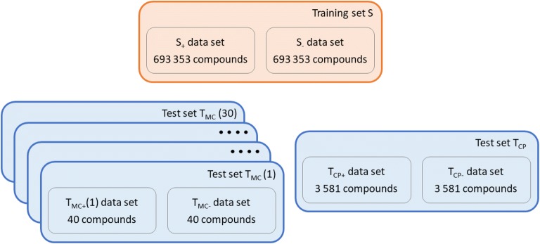
The training data set S consists of two subsets: S+ contains ES structures and S- contains HS structures (Fig. 1, Additional file 1). While ES molecules can be readily obtained, for example, from the ZINC database of purchasable compounds [56, 57], no equivalent database of HS molecules exists. However, HS molecules can be designed by Nonpher [58], a method based on a molecular morphing approach [59]. In Nonpher, a starting molecule is gradually transformed into a more complex compound using small structural perturbations, such as the addition or removal of an atom or a bond. To prevent the creation of overly complex structures, four complexity indices (Bertz [34], Whitlock [35], BC [36] and SMCM [37]) are monitored and once their respective thresholds (Additional file 2: Table S1) are exceeded, Nonpher is stopped.
Fig. 1.
Data set summary. Training set was used to derive SYBA scores, as well as to train a random forest classifier. Training set consists of 693 353 molecules randomly selected from the ZINC15 database [57] that are considered to be ES (S+ data set) and of the same number of HS molecules generated by Nonpher [58] (S− data set). Two test sets were used to compare the performance of SYBA, a random forest, SAScore [45] and SCScore [43]. Manually curated test set (TMC) contains 40 compounds (TMC- data set) considered to be HS by experienced medicinal chemists [58] supplemented by 40 ES compounds randomly selected from the ZINC15 database (TMC+ data set). 30 TMC data set instances differing in TMC+ compounds were constructed. Computationally picked test set (TCP) consists of 3 581 HS compounds that were obtained from the GDB-17 database [61] (TCP- data set) complemented by the same number of compounds randomly selected from the ZINC15 database (TCP+ data set)
Using Nonpher, 693 353 HS molecules were generated and they form the S- data set. The S+ data set, containing ES compounds, is formed by the same number of molecules randomly chosen (excluding natural products) from the ZINC15 database [57] so that their distribution of the number of heavy atoms is the same as in the S- data sets. Every S+ and S- molecule was fragmented using the Morgan fingerprint function in the RDKit toolkit [60]. Fragments with the radius of 4 and smaller, corresponding to radial ECFP8 [46] fragments, were used. This type of fragments consists of a central atom and atoms distant from the central atom up to four bonds. Besides ECFP8 fragments, the number of stereocenters was also included into SYBA as the molecules with more stereocenters are typically more difficult to synthesize. The stereo score is based, similarly to the fragment score, on the analysis of the number of stereocenters in the training set S. To obtain the stereo score, molecules were divided into 6 bins differing by the number of stereocenters (0, 1, 2, 3, 4 and 5+) and individual score contributions were calculated from Eq. 7.
Test set construction
SYBA performance could have been assessed using a test set created in a similar way as the training set S, i.e. using HS compounds generated by Nonpher. However, such test set would be clearly biased towards chemical space covered by Nonpher. Therefore, two test sets were constructed in a conceptually different manner. First test set, further denoted as TMC, was manually curated from the literature, second test set, referred to as TCP, was computationally picked from the ZINC15 [57] and GDB17 databases [61].
HS compounds in TMC (denoted as TMC−) were obtained by the analysis [58] of 296 published compounds assessed by experienced medicinal chemists [41, 45, 62, 63]. Based on original chemists’ scores, the final TMC- data set of 40 HS compounds was assembled. A complementary TMC+ data set consists of 40 ES compounds selected from the ZINC15 database [57] in such a way that the distribution of the number of their heavy atoms is the same as in the TMC- data set. Because small TMC size may bias the results, 30 different TMC data set instances were generated using the same 40 TMC- compounds, but different 40 TMC+ compounds (Additional file 3).
HS compounds in the TCP test set (Additional file 4), denoted as TCP-, were obtained by the analysis of the publicly available subset of 50 M molecules from the GDB-17 database [61]. Only molecules exceeding thresholds (Additional file 2: Table S1) of all monitored complexity indices (Bertz [34], Whitlock [35], BC [36] and SMCM [37]) were considered to be HS. In total, 3 581 molecules form the TCP- data set. A complementary TCP+ data set consists of the same number of compounds randomly selected from the ZINC15 database [57] that follow the same size distribution as HS compounds and that, in addition, do not exceed any of the aforedescribed complexity indices. Data sets used in the present work are summarized in Fig. 1.
Performance evaluation
The performance of classification models studied in the present work was assessed by four different metrics: the classification accuracy (Acc), sensitivity (SN), specificity (SP) and area under the ROC curve (AUC). Acc gives the percentage of correctly classified samples regardless of their class.
| 8 |
where true positives (TP) are ES compounds predicted by a model to be ES, true negatives (TN) are HS compounds predicted to be HS, false positives (FP) are HS compounds predicted to be ES and false negatives (FN) are ES compounds predicted to be HS. The accuracy can also be evaluated for positive and negative classes independently leading to SN and SP. SN is the percentage of correctly predicted positive class compounds, while the percentage of correctly predicted negative class compounds is known as SP.
| 9 |
| 10 |
SN and SP can be combined in the receiver operating characteristic (ROC) curve that is the graphical representation of the trade-off between true positive rate (given as SN) and false positive rate (given as 1 − SP) over all possible thresholds (Fig. 2). The area under the ROC curve (AUC) is the quantitative measure of the performance of a classifier and is equal to the probability that a classifier will rank a randomly chosen positive example higher than a randomly chosen negative example. A random classifier has AUC of 0.5, while AUC for a perfect classifier is equal to 1.
Fig. 2.
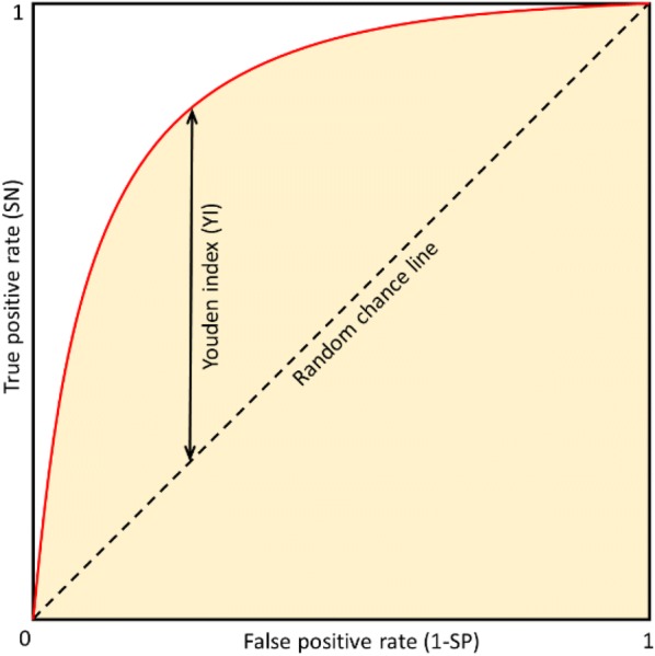
ROC curve and Youden index. The ROC curve (red line) is the dependency of true positive rate (it equals to SN) on false positive rate (it equals to 1-SP) at various thresholds. The random chance line represents a classifier that assigns examples into individual classes randomly. Orange shaded area represents the area under the ROC curve (AUC). The larger the AUC, the better is the overall performance of the classifier. Youden index (YI) is the point on the ROC curve that is farthest from the random chance line along the SN axis
Random forest classification, SAScore and SCScore
Because of its wide adoption in various cheminformatics applications [58, 64–66], the random forest (RF) classifier with compounds encoded by 1024-bits long Morgan fingerprint with radius 2 was used as a baseline method with which SYBA, SAScore [45] and SCScore [43] were compared. The RF classifier was implemented in Scikit-learn [67]. Two RF hyperparameters were optimized: the number of trees (50, 100, 300 and 500) and the maximum number of features considered when looking for the best split (10% out of 1024 = 102, 25% = 256, 50% = 512, 75% = 768, 100% = 1024, and ). For each pair of hyperparameters, RF model was trained using the training set S and the prediction accuracy was evaluated on the test set TCP (Additional file 2: Table S2, Figures S2–S8). The setting used in this work (100 trees and 32 features) represents the best trade-off between computational efficiency and prediction accuracy [64]. RF was trained using the training set S (Fig. 1). SAScore was calculated by the RDKit toolkit [60]. SCScore code was downloaded from the public GitHub repository [68].
Classification thresholds
In SYBA, more positive value means a higher probability that the compound is ES and more negative value indicates a higher probability that the compound is HS (Eq. 4). The threshold value of zero is used to distinguish between ES and HS compounds. For SAScore, the recommended value of 6.0 [45] was used as a threshold. In RF, the final prediction is based on a number of decision trees that predict either of classes. Here, 0.5 is used as a threshold, i.e., if more decision trees predict ES than HS class, a compound is classified as ES and vice versa. For SCScore [43], no threshold was suggested by the authors. In such case, the threshold can be identified by the analysis of the ROC curve. A frequently used measure that enables the selection of an optimal threshold is the Youden index (YI) [69, 70]. YI is defined as
| 11 |
and ranges between 0 and 1 (Fig. 2). The optimal threshold value is selected by maximizing YI, i.e., by maximizing the sum of SN and SP.
Statistical comparison of model performance
The performance of studied classification models was compared using non-parametric Cochran’s Q test [71], an omnibus test for testing for differences between three or more machine learning models. In the case of the statistically significant result of Cochran’s Q test, differing pairs of classification models were identified by McNemar’s post hoc paired test [72] with Benjamini–Hochberg false discovery rate adjustment [73]. McNemar’s test checks if the distribution of disagreements between two methods is imbalanced. The statistical significance for all tests in the present work was assessed at the significance level α = 0.05.
Results and discussion
Chemical space covered by SYBA data sets
The examples of training set compounds are given in Additional file 2: Figures S9–S12. In total, 3 439 074 ECFP8 fragments were obtained for ES compounds and 23 447 524 fragments for HS compounds. 458 040 fragments are common for both S + and S- subsets. 55.0% of S+ fragments and 91.7% of S− fragments are present only once in the whole data set S (singletons). Typical ES and HS fragments are shown in Figs. 3 and 4, fragments with very low SYBA in Additional file 2: Figure S13 and compounds containing these fragments in Additional file 2: Figure S14.
Fig. 3.
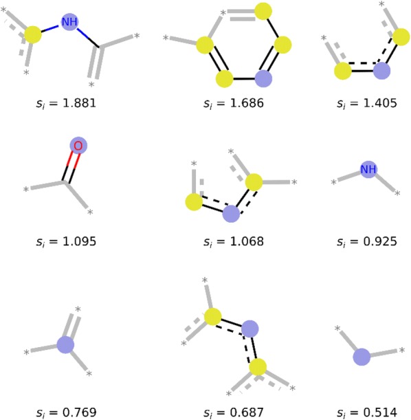
ES fragments enriched in the S+ data set. Nine fragments that are most frequent in the S+ data set and, at the same time, least frequent in the S- data set. si is SYBA fragment score. Blue circles represent each fragment central atom, yellow circles represent aromatic atoms. Fragment images were generated by the RDKit function DrawMorganEnvs()
Fig. 4.
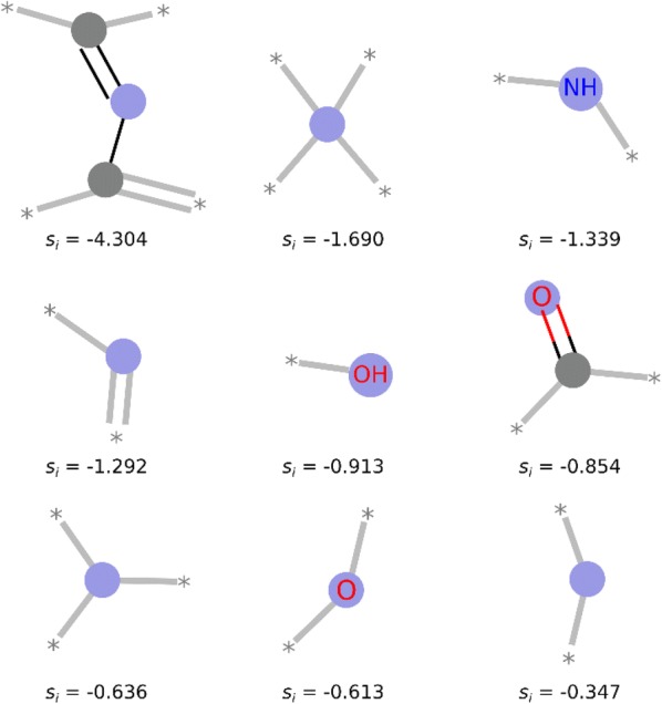
HS fragments enriched in the S- data set. Nine fragments that are most frequent in the S- data set and, at the same time, least frequent in the S+ data set. si is SYBA fragment score. Blue circles represent fragment central atom, gray circles represent aliphatic ring atoms. Fragment images were generated by the RDKit function DrawMorganEnvs()
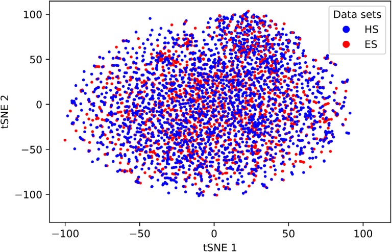
Though the number of fragments in HS compounds is much larger than in ES compounds, chemical space is equally covered by both HS and ES molecules and there is no bias towards HS compounds (Fig. 5).
Fig. 5.
Chemical space coverage by ES and HS training set compounds. 3000 ES and 3000 HS compounds were randomly selected from the training set and each compound was encoded by 1024 bits long ECFP4 fingerprint. The dimensionality of the input space was reduced by SVD to 500 components that explain 85% of the variance in the data
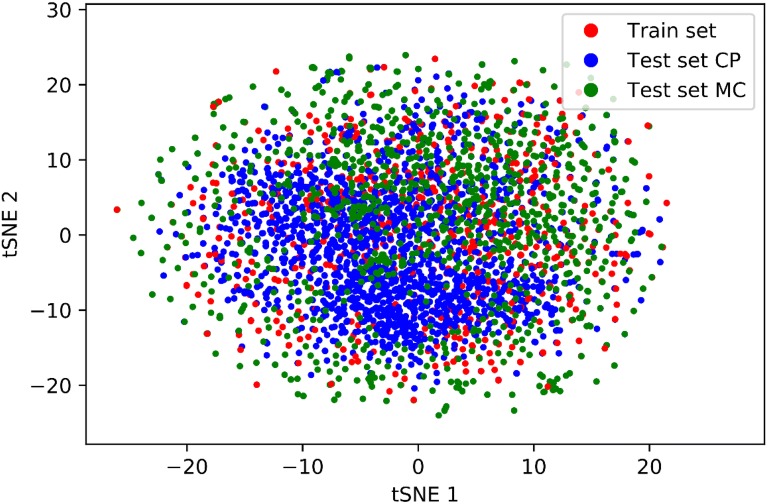
The visualization of chemical space (Fig. 6) covered by S, TCP and TMC compounds shows that test set compounds lie within chemical space of training compounds. The examples of TCP and TMC compounds are given in Additional file 2: Figures S15–S21.
Fig. 6.
Chemical space coverage by training set S and test sets TCP and TMC. TMC data set consists of 40 HS compounds and 1200 ES compounds, from S and TCP data sets random samples of 1240 compounds were generated. Each compound was encoded by 1024 bits long ECFP4 fingerprint. The dimensionality of the input space was reduced by SVD to 500 components that explain 88% of the variance in the data
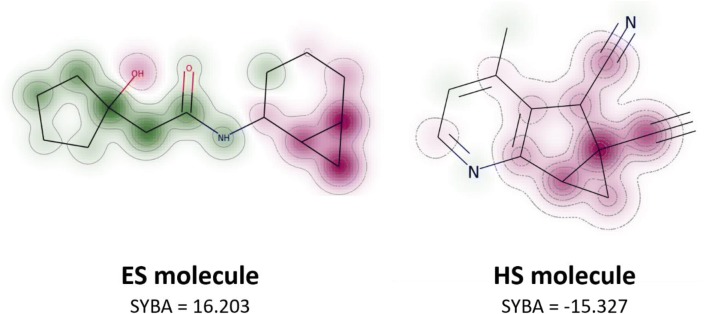
SYBA also enables the visualization and interpretation of fragment score contributions. Each SYBA fragment score can be projected to the corresponding fragment root atom and this projection can be used to analyze which fragments contribute unfavorably to molecule synthetic accessibility (Fig. 7).
Fig. 7.
SYBA fragment score visualization. Fragment score is projected on the fragment root atom and the whole molecule is visualized as a similarity map [74]. The more frequent the fragment is in the S+ data set compared to the S- data set, the greener is its central atom. Similarly, the more frequent the fragment is in the S- data set compared to the S+ data set, the redder is its central atom. This visualization enables to analyze the contributions of the individual parts of the molecule to its synthetic accessibility. In the HS molecule, the quaternary carbon is most problematic. Another substructure decreasing compound synthetic accessibility is a fused cyclopropane ring as can be observed both in ES and HS compounds
Classifier performance on manually curated test set
The differences in classification of TMC (Fig. 1) compounds using SYBA, SAScore and RF with default thresholds are statistically significant. The Cochran’s Q test p value is 2 × 10⁻⁵ for the TMC test set with the smallest SYBA AUC. The results of the corresponding McNemar’s paired tests [72] are summarized in Table 1. While RF and SYBA do not differ significantly, both RF and SYBA yield significantly better results than SAScore.
Table 1.
The results of McNemar’s two-sided paired tests for the TMC test set with the smallest SYBA AUC (AUC = 0.830)
| Adjusted p-value | |
|---|---|
| RF vs. SAScore | 0.002 |
| RF vs. SYBA | 1.000 |
| SAScore vs. SYBA | 0.001 |
The default threshold values were used (0.0 for SYBA, 0.5 for RF, and 6.0 for SAScore). The p-values were adjusted using Benjamini–Hochberg method
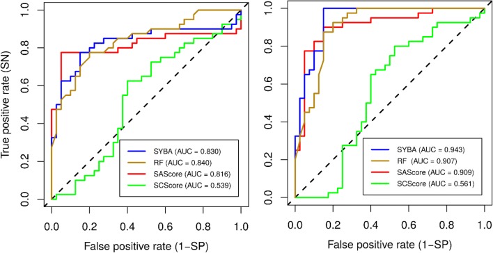
The quality measures of the classification of the compounds in the manually curated TMC test set, averaged over 30 TMC instances, are summarized in Table 2. The corresponding confusion matrices are reported in Additional file 2: Panel S1 and Panel S2 and ROC curves are shown in Fig. 8.
Table 2.
The performance of classification models for the manually curated TMC test set
| Model | AUC | Acc | SN | SP | Threshold |
|---|---|---|---|---|---|
| Default threshold | |||||
| SYBA | 0.903 | 0.844 | 0.913 | 0.775 | 0.0 |
| SAScore | 0.865 | 0.617 | 0.934 | 0.300 | 6.0 |
| RF | 0.875 | 0.819 | 0.863 | 0.775 | 0.5 |
| Optimized threshold | |||||
| SYBA | 0.903 | 0.871 | 0.902 | 0.840 | 19.1 |
| SAScore | 0.865 | 0.859 | 0.799 | 0.919 | 3.9 |
| SCScore | 0.528 | 0.601 | 0.707 | 0.496 | 3.7 |
| RF | 0.875 | 0.842 | 0.855 | 0.828 | 0.6 |
Quality measures AUC, Acc, SN and SP, as well as thresholds, are reported as their average values over 30 TMC instances
Fig. 8.
The ROC curves of classification models for the manually curated TMC test set. Out of 30 possible TMC instances, ROC curves of the TMC test set with the smallest (left) and largest (right) SYBA AUC are shown
In terms of Acc, the best performing model is SYBA followed by RF and SAScore. While SYBA and RF sensitivity and specificity are well balanced, SAScore shows high sensitivity (SN = 0.934, i.e., on average 93.4% of ES compounds are predicted as ES), while its specificity (i.e., the ability to correctly classify HS compounds) is rather low (SP = 0.300). The observed high sensitivity of SAScore is not surprising as only 0.2% of ZINC structures have SAScore greater than 6.0 and out of these, only lower units were selected into the TMC+ set.
For optimized thresholds, the differences between SYBA, SAScore and RF are again statistically significant (Cochran’s Q test p-value is 2 × 10⁻¹⁴ for the TMC test set with the smallest SYBA AUC). However, McNemar’s paired test (Table 3) identifies significant differences only between SCScore and other methods meaning that SAScore results improve significantly upon threshold optimization.
Table 3.
The results of McNemar’s two-sided paired tests for the TMC test set with the smallest SYBA AUC (AUC = 0.830)
| Adjusted p-value | |
|---|---|
| RF vs. SAScore | 0.164 |
| RF vs. SCScore | 2 × 10⁻⁶ |
| RF vs. SYBA | 0.687 |
| SAScore vs. SCScore | 1 × 10⁻⁸ |
| SAScore vs. SYBA | 0.466 |
| SCScore vs. SYBA | 2 × 10⁻⁶ |
The optimized threshold values were used (27.7 for SYBA, 0.5 for RF, 3.7 for SAScore, and 4.0 for SCScore). The p-values were adjusted using Benjamini–Hochberg method
In terms of performance measures (Table 2), the most accurate classifiers are SYBA, RF and SAScore followed afar by SCScore. Notable is the improvement of SAScore SP by 0.619 compared to the default threshold. The increase in SAScore SP comes, however, at the cost of SN that decreases by 0.135. The worst performing model, SCScore, is only slightly better (AUC = 0.528) than a random model. However, because TMC+ and TMC− data sets consist of only 40 compounds each, the results must be interpreted with caution as small changes in confusion matrices lead to relatively large changes in reported metrics.
Classifier performance on computationally picked test set
Even stronger evidence of the differences between the models is provided by the classification of compounds in the large computationally picked TCP test set (Fig. 1). Using the default thresholds, the differences between the classifiers are statistically significant (Cochran’s Q test p-value < 10−16) and all classifiers differ significantly (Table 4).
Table 4.
The results of McNemar’s two-sided paired tests for the TCP test set
| Adjusted p-value | |
|---|---|
| RF vs. SAScore | < 10−16 |
| RF vs. SYBA | < 10−16 |
| SAScore vs. SYBA | < 10−16 |
The default threshold values were used (0.0 for SYBA, 0.5 for RF, and 6.0 for SAScore). The p-values were adjusted using Benjamini–Hochberg method
When used with their default thresholds, both SYBA and RF are more accurate than SAScore (Table 5, Additional file 2: Panel S3). Low observed SAScore accuracy (Acc = 0.665) is caused by its low specificity when almost 70% of HS compounds are predicted to be ES (Table 5).
Table 5.
The performance of classification models for the computationally picked TCP test set
| Model | AUC | Acc | SN | SP | Threshold |
|---|---|---|---|---|---|
| Default threshold | |||||
| SYBA | 0.903 | 0.962 | 0.925 | 1.000 | 0.0 |
| SAScore | 0.999 | 0.665 | 0.999 | 0.331 | 6.0 |
| RF | 0.995 | 0.892 | 0.784 | 0.999 | 0.5 |
| Optimized threshold | |||||
| SYBA | 0.998 | 0.988 | 0.985 | 0.991 | − 18.6 |
| SAScore | 0.999 | 0.990 | 0.986 | 0.993 | 4.5 |
| SCScore | 0.641 | 0.612 | 0.499 | 0.725 | 3.1 |
| RF | 0.995 | 0.973 | 0.960 | 0.986 | 0.2 |
Cochran’s Q test identifies significant differences (p-value < 10−16) also if classifiers are used with the optimized thresholds. While statistically significant differences were detected within RF/SAScore and RF/SYBA pairs (Table 6), the effect size is still rather small (Table 5). However, the difference between SCScore and all other methods is statistically significant and large (Tables 5 and 6). No statistically significant difference was observed between SYBA and SAScore meaning that these two methods yield comparable results.
Table 6.
The results of McNemar’s two-sided paired tests for the TCP test set
| Adjusted p-value | |
|---|---|
| RF vs. SAScore | 4 × 10⁻¹⁵ |
| RF vs. SCScore | < 10−16 |
| RF vs. SYBA | 2 × 10⁻¹⁴ |
| SAScore vs. SCScore | < 10−16 |
| SAScore vs. SYBA | 0.474 |
| SCScore vs. SYBA | < 10−16 |
The optimized values of threshold (− 18.6 for SYBA, 0.2 for RF, 4.5 for SAScore, 3.1 for SCScore) were used. p-values were adjusted using Benjamini–Hochberg method
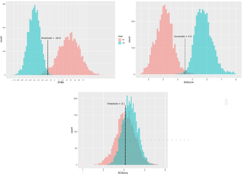
Compared to its default threshold of 6.0, SAScore specificity increases by 0.662 (Table 5) when the threshold is shifted to the optimal value of 4.5 (Fig. 10). At this threshold, SAScore is on par with SYBA and RF methods (Table 5). However, SYBA retains its high performance over much broader range of threshold values than SAScore (Additional file 2: Figure S1).
Fig. 10.
SYBA, SAScore and SCScore histograms of ES and HS compounds in the computationally picked TCP test set. The positions of optimal thresholds are shown. SAScore recommended threshold of 6.0 leads to a large number of FP (Additional file 2: Panel S3). If the threshold is moved to its optimal value of 4.5, SAScore specificity increases from 0.317 to 0.994, i.e. by 0.677
High performance of SYBA, RF and SAScore is also evident from their AUC that is close to one (Fig. 9, Table 5). On the other hand, SCScore fails to distinguish between ES and HS compounds as can be deduced from its ROC curve (Fig. 9). In its optimal threshold of 3.1, SCScore predicts a majority of TCP compounds as HS (Fig. 10, Additional file 2: Panel S3).
Fig. 9.
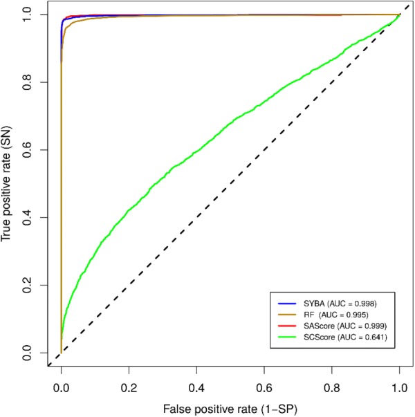
ROC curves of classification models for the TCP test set
In addition to the TMC and TCP test sets, the performance of SAScore and SCScore was also assessed using the training set S, as this data set was not used for their parametrization. Classification results are shown in Table 7 and Fig. 11, confusion matrices are available in Additional file 2: Panel S4.
Table 7.
The performance of classification models for the training set S
| Model | AUC | Acc | SN | SP | Threshold |
|---|---|---|---|---|---|
| Default threshold | |||||
| SAScore | 0.981 | 0.767 | 0.998 | 0.536 | 6.0 |
| Optimized threshold | |||||
| SAScore | 0.981 | 0.933 | 0.935 | 0.932 | 4.4 |
| SCScore | 0.667 | 0.623 | 0.564 | 0.682 | 3.7 |
Fig. 11.
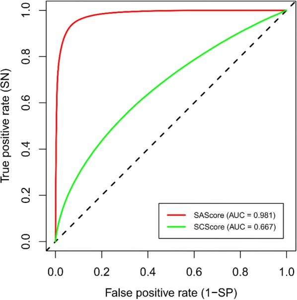
ROC curves of classification models for the training set S
In agreement with previous experiments on the TMC and TCP test sets, SAScore is able to distinguish between ES and HS compounds more accurately than SCScore. However, to achieve the best performance, SAScore classification threshold must be shifted from its default value of 6.0 to the optimal value of 4.4. At this threshold, SAScore is both highly sensitive and specific, while SCScore is, using its optimal threshold of 3.7, sensitive and specific only moderately.
The observed poor performance of SCScore in all data sets may follow from the fact that SCScore differs conceptually from other methods tested in the present work. In SCScore, the problem of predicting synthetic complexity is reformulated as the analysis of reactions consisting of reactant-product pairs and SCScore correlates with a number of reaction steps. It means that, contrary to SYBA and SAScore, SCScore captures synthetic feasibility of compounds, not structural complexity. In SCScore derivation, each molecule is analyzed as a whole in the context of all molecules and reactions as they appear in the Reaxys database [44]. Thus, SCScore is biased [43] by the types of reactants and products in the Reaxys database. Therefore, we hypothesize that the unsatisfactory results of SCScore are caused by the fact that compounds in our data sets come from chemical subspace insufficiently covered by Reaxys compounds.
Conclusions
In the present work, SYBA method for the classification of organic compounds as easy- and hard-to-synthesize is described. SYBA is an additive fragment-based approach meaning that the compound is decomposed into individual substructure fragments, each fragment is assigned its respective SYBA fragment score and these are summed to obtain the final SYBA score. The fragment scores were derived by the Bayesian analysis of the frequency of ECFP8 fragments occurring in the database of ES compounds, that were randomly chosen from the ZINC15 database [57], and HS compounds, that were generated using the Nonpher approach [58]. Because SYBA was derived from ECFP8 fragments that utilize only molecular connectivity and no 3D information, the influence of stereochemistry on synthetic accessibility is not accounted for. However, apart from ECFP8 fragments, the number of stereocenters is included in SYBA calculation and the compounds with many stereocenters are penalized. If the SYBA score is positive, the compound is considered to be ES and vice versa. While SYBA score can theoretically assume values between plus and minus infinity, a majority of compounds will have SYBA score between − 100 and +100 in real applications. It must be stressed here that the absolute value of the SYBA score is the measure of the confidence of the prediction and not of the degree of the synthetic accessibility.
SYBA was compared with other two recent classification methods, SAScore [45] and SCScore [43]. As a baseline for the comparison, RF/ECFP4 classifier was used due to its wide adoption in many cheminformatics applications. All methods were assessed using accuracy, sensitivity, specificity and area under the ROC curve. While SYBA and RF provide similar performance, we recommend to use SYBA due to its smaller complexity, lower computational demands and more straightforward analysis of the individual fragment contributions. SYBA outperforms SAScore when this is used with the threshold of 6.0 proposed by the authors [45]. However, if the SAScore threshold is changed to the value of ~ 4.5, the accuracy of SYBA and SAScore becomes comparable. Therefore, to reduce the number of false positives in workflows that utilize SAScore, we recommend to decrease the SAScore threshold to ~ 4.5. SYBA, RF and SAScore substantially outperform SCScore. The observed weak performance of SCScore can be, in our opinion, attributed to the fact that our test set compounds come from a part of chemical space that is insufficiently covered by Reaxys compounds used to derive SCScore. The SYBA fragment scores can be mapped [74] onto a molecule and used for the analysis of the contribution of its individual substructures to the overall synthetic accessibility.
SYBA can be used to quickly rank large molecular data sets that originate, for example, from de novo molecular design. However, SYBA is conceptually based on the notion that a compound can be categorized as easy- and hard-to-synthesize. As the synthetic accessibility is a vaguely defined term, SYBA’s simplifying approach, though accurate enough, cannot compete with more sophisticated synthetic path-reconstruction methods that enable the incorporation of other factors such as the availability of starting materials, reaction yields or a price aspect. In the end, the definitive assessment of synthetic accessibility is in the hands of experienced organic chemists.
Supplementary information
Additional file 1. Training set S. It consists of 693 353 ES compounds selected from the ZINC15 database and of 693 353 ES compounds generated by Nonpher.
Additional file 2. This supporting document contains the detailed description of the SYBA score derivation, threshold values of complexity indices, RF hyperparameter optimization results, the dependence of the accuracy of the classification of TCP compounds on SYBA and SAScore thresholds, examples of correctly predicted and mispredicted S, TMC and TCP compounds, fragments with very low SYBA contributions and HS compounds containing these fragments, and confusion matrices of the classification of TMC, TCP and S data sets.
Additional file 3. Manually curated test set (TMC). It consists of 40 HS compounds manually selected from scientific papers and of 30 ES sets, each of them contains 40 compounds selected from the ZINC15 database.
Additional file 4. Computationally picked test set (TCP). It consists of 3 581 HS compounds that were obtained from the GDB-17 database complemented by the same number of compounds randomly selected from the ZINC15 database.
Acknowledgements
Computational resources were supplied by the project “e-Infrastruktura CZ” (e-INFRA LM2018140) provided within the program Projects of Large Research, Development and Innovations Infrastructures.
Abbreviations
- Acc
Accuracy
- AUC
Area under the ROC curve
- ES
Easy-to-synthesize
- HS
Hard-to-synthesize
- MW
Molecular weight
- RF
Random forest
- ROC
Receiver operating characteristic
- S
Training set
- SN
Sensitivity
- SP
Specificity
- SVD
Singular value decomposition
- SYBA
SYnthetic Bayesian Accessibility
- TCP
Computationally picked test set
- TMC
Manually curated test set
- YI
Youden index
Authors’ contributions
MV, MK and DS conceptualized the problem. MV was responsible for method development, implementation and validation. MV also maintains the SYBA GitHub repository. MK derived SYBA and IČ took part in method testing. DS supervised the study, performed statistical analyses and prepared the manuscript with the active participation of MV, MK and IČ. All authors read and approved the final manuscript.
Funding
This work was supported from the Ministry of Education of the Czech Republic (RVO 68378050-KAV-NPUI and LM2018130). IČ research was further supported by a specific university research (MSMT No. 20/2015). MK was supported by the project “Center for Tumor Ecology-Research of the Cancer Microenvironment Supporting Cancer Growth and Spread” (Reg. No. CZ.02.1.01/0.0/0.0/16_019/0000785) within the Operational Programme Research, Development and Education.
Availability of data and materials
The code used to train and benchmark SYBA model is available from https://github.com/lich-uct/syba repository. Nonpher is available from https://github.com/lich-uct/nonpher.
Competing interests
The authors declare that they have no competing interests.
Footnotes
Publisher's Note
Springer Nature remains neutral with regard to jurisdictional claims in published maps and institutional affiliations.
Contributor Information
Milan Voršilák, Email: milan.vorsilak@img.cas.cz.
Michal Kolář, Email: kolarmi@img.cas.cz.
Ivan Čmelo, Email: ivan.cmelo@vscht.cz.
Daniel Svozil, Email: daniel.svozil@vscht.cz.
Supplementary information
Supplementary information accompanies this paper at 10.1186/s13321-020-00439-2.
References
- 1.Bohacek RS, McMartin C, Guida WC. The art and practice of structure-based drug design: a molecular modeling perspective. Med Res Rev. 1996;16(1):3–50. doi: 10.1002/(SICI)1098-1128(199601)16:1<3::AID-MED1>3.0.CO;2-6. [DOI] [PubMed] [Google Scholar]
- 2.Polishchuk PG, Madzhidov TI, Varnek A. Estimation of the size of drug-like chemical space based on GDB-17 data. J Comput Aided Mol Des. 2013;27(8):675–679. doi: 10.1007/s10822-013-9672-4. [DOI] [PubMed] [Google Scholar]
- 3.Ertl P. Cheminformatics analysis of organic substituents: identification of the most common substituents, calculation of substituent properties, and automatic identification of drug-like bioisosteric groups. J Chem Inf Comput Sci. 2003;43(2):374–380. doi: 10.1021/ci0255782. [DOI] [PubMed] [Google Scholar]
- 4.Reymond JL, van Deursen R, Blum LC, Ruddigkeit L. Chemical space as a source for new drugs. Medchemcomm. 2010;1(1):30–38. [Google Scholar]
- 5.Llanos EJ, Leal W, Luu DH, Jost J, Stadler PF, Restrepo G. Exploration of the chemical space and its three historical regimes. Proc Natl Acad Sci U S A. 2019;116(26):12660–12665. doi: 10.1073/pnas.1816039116. [DOI] [PMC free article] [PubMed] [Google Scholar]
- 6.Karlov DS, Sosnin S, Tetko IV, Fedorov MV. Chemical space exploration guided by deep neural networks. Rsc Advances. 2019;9(9):5151–5157. doi: 10.1039/c8ra10182e. [DOI] [PMC free article] [PubMed] [Google Scholar]
- 7.Gromski PS, Henson AB, Granda JM, Cronin L. How to explore chemical space using algorithms and automation. Nat Rev Chem. 2019;3(2):119–128. [Google Scholar]
- 8.Walters WP. Virtual chemical libraries. J Med Chem. 2019;62(3):1116–1124. doi: 10.1021/acs.jmedchem.8b01048. [DOI] [PubMed] [Google Scholar]
- 9.Franzini RM, Neri D, Scheuermann J. DNA-encoded chemical libraries: advancing beyond conventional small-molecule libraries. Acc Chem Res. 2014;47(4):1247–1255. doi: 10.1021/ar400284t. [DOI] [PubMed] [Google Scholar]
- 10.Lopez-Vallejo F, Caulfield T, Martinez-Mayorga K, Giulianotti MA, Nefzi A, Houghten RA, Medina-Franco JL. Integrating virtual screening and combinatorial chemistry for accelerated drug discovery. Comb Chem High Throughput Screen. 2011;14(6):475–487. doi: 10.2174/138620711795767866. [DOI] [PubMed] [Google Scholar]
- 11.Hoffmann T, Gastreich M. The next level in chemical space navigation: going far beyond enumerable compound libraries. Drug Discov Today. 2019;24(5):1148–1156. doi: 10.1016/j.drudis.2019.02.013. [DOI] [PubMed] [Google Scholar]
- 12.van Hilten N, Chevillard F, Kolb P. Virtual compound libraries in computer-assisted drug discovery. J Chem Inf Model. 2019;59(2):644–651. doi: 10.1021/acs.jcim.8b00737. [DOI] [PubMed] [Google Scholar]
- 13.Schneider G, Fechner U. Computer-based de novo design of drug-like molecules. Nat Rev Drug Discov. 2005;4(8):649–663. doi: 10.1038/nrd1799. [DOI] [PubMed] [Google Scholar]
- 14.Loving K, Alberts I, Sherman W. Computational approaches for fragment-based and de novo design. Curr Top Med Chem. 2010;10(1):14–32. doi: 10.2174/156802610790232305. [DOI] [PubMed] [Google Scholar]
- 15.Medina-Franco JL, Martinez-Mayorga K, Meurice N. Balancing novelty with confined chemical space in modern drug discovery. Expert Opin Drug Discov. 2014;9(2):151–165. doi: 10.1517/17460441.2014.872624. [DOI] [PubMed] [Google Scholar]
- 16.Schneider P, Schneider G. De Novo design at the edge of Chaos. J Med Chem. 2016;59(9):4077–4086. doi: 10.1021/acs.jmedchem.5b01849. [DOI] [PubMed] [Google Scholar]
- 17.Kutchukian PS, Shakhnovich EI. De novo design: balancing novelty and confined chemical space. Expert Opin Drug Discov. 2010;5(8):789–812. doi: 10.1517/17460441.2010.497534. [DOI] [PubMed] [Google Scholar]
- 18.Hartenfeller M, Schneider G. De novo drug design. Methods Mol Biol. 2011;672:299–323. doi: 10.1007/978-1-60761-839-3_12. [DOI] [PubMed] [Google Scholar]
- 19.Hartenfeller M, Proschak E, Schuller A, Schneider G. Concept of combinatorial de novo design of drug-like molecules by particle swarm optimization. Chem Biol Drug Des. 2008;72(1):16–26. doi: 10.1111/j.1747-0285.2008.00672.x. [DOI] [PubMed] [Google Scholar]
- 20.Vinkers HM, de Jonge MR, Daeyaert FF, Heeres J, Koymans LM, van Lenthe JH, Lewi PJ, Timmerman H, Van Aken K, Janssen PA. SYNOPSIS: SYNthesize and OPtimize System in Silico. J Med Chem. 2003;46(13):2765–2773. doi: 10.1021/jm030809x. [DOI] [PubMed] [Google Scholar]
- 21.Hartenfeller M, Zettl H, Walter M, Rupp M, Reisen F, Proschak E, Weggen S, Stark H, Schneider G. DOGS: reaction-driven de novo design of bioactive compounds. PLoS Comput Biol. 2012;8(2):e1002380. doi: 10.1371/journal.pcbi.1002380. [DOI] [PMC free article] [PubMed] [Google Scholar]
- 22.Schneider G, Lee ML, Stahl M, Schneider P. De novo design of molecular architectures by evolutionary assembly of drug-derived building blocks. J Comput Aided Mol Des. 2000;14(5):487–494. doi: 10.1023/a:1008184403558. [DOI] [PubMed] [Google Scholar]
- 23.Fechner U, Schneider G. Flux (1): a virtual synthesis scheme for fragment-based de novo design. J Chem Inf Model. 2006;46(2):699–707. doi: 10.1021/ci0503560. [DOI] [PubMed] [Google Scholar]
- 24.Chen H, Engkvist O, Wang Y, Olivecrona M, Blaschke T. The rise of deep learning in drug discovery. Drug Discov Today. 2018;23(6):1241–1250. doi: 10.1016/j.drudis.2018.01.039. [DOI] [PubMed] [Google Scholar]
- 25.Hessler G, Baringhaus KH. Artificial intelligence in drug design. Molecules. 2018;23(10):2520. doi: 10.3390/molecules23102520. [DOI] [PMC free article] [PubMed] [Google Scholar]
- 26.Xu Y, Lin K, Wang S, Wang L, Cai C, Song C, Lai L, Pei J. Deep learning for molecular generation. Future Med Chem. 2019;11(6):567–597. doi: 10.4155/fmc-2018-0358. [DOI] [PubMed] [Google Scholar]
- 27.Popova M, Isayev O, Tropsha A. Deep reinforcement learning for de novo drug design. Sci Adv. 2018;4(7):7885. doi: 10.1126/sciadv.aap7885. [DOI] [PMC free article] [PubMed] [Google Scholar]
- 28.Olivecrona M, Blaschke T, Engkvist O, Chen H. Molecular de-novo design through deep reinforcement learning. J Cheminform. 2017;9(1):48. doi: 10.1186/s13321-017-0235-x. [DOI] [PMC free article] [PubMed] [Google Scholar]
- 29.Blaschke T, Olivecrona M, Engkvist O, Bajorath J, Chen H. Application of generative autoencoder in de novo molecular design. Mol Inform. 2018;37(1–2):1700123. doi: 10.1002/minf.201700123. [DOI] [PMC free article] [PubMed] [Google Scholar]
- 30.Segler MHS, Kogej T, Tyrchan C, Waller MP. Generating focused molecule libraries for drug discovery with recurrent neural networks. ACS Cent Sci. 2018;4(1):120–131. doi: 10.1021/acscentsci.7b00512. [DOI] [PMC free article] [PubMed] [Google Scholar]
- 31.Gupta A, Müller AT, Huisman BJ, Fuchs JA, Schneider P, Schneider G. Generative recurrent networks for de novo drug design. Mol Inform. 2018;37(1–2):1700111. doi: 10.1002/minf.201700111. [DOI] [PMC free article] [PubMed] [Google Scholar]
- 32.Merk D, Friedrich L, Grisoni F, Schneider G. De novo design of bioactive small molecules by artificial intelligence. Mol Inform. 2018;37(1–2):1700153. doi: 10.1002/minf.201700153. [DOI] [PMC free article] [PubMed] [Google Scholar]
- 33.Mendez-Lucio O, Medina-Franco JL. The many roles of molecular complexity in drug discovery. Drug Discov Today. 2017;22(1):120–126. doi: 10.1016/j.drudis.2016.08.009. [DOI] [PubMed] [Google Scholar]
- 34.Bertz SH. The first general index of molecular complexity. J Am Chem Soc. 1981;103(12):3599–3601. [Google Scholar]
- 35.Whitlock HW. On the structure of total synthesis of complex natural products. J Organic Chem. 1998;63(22):7982–7989. [Google Scholar]
- 36.Barone R, Chanon M. A new and simple approach to chemical complexity application to the synthesis of natural products. J Chem Inf Comp Sci. 2001;41(2):269–272. doi: 10.1021/ci000145p. [DOI] [PubMed] [Google Scholar]
- 37.Allu TK, Oprea TI. Rapid evaluation of synthetic and molecular complexity for in silico chemistry. J Chem Inf Model. 2005;45(5):1237–1243. doi: 10.1021/ci0501387. [DOI] [PubMed] [Google Scholar]
- 38.Selzer P, Roth HJ, Ertl P, Schuffenhauer A. Complex molecules: do they add value? Curr Opin Chem Biol. 2005;9(3):310–316. doi: 10.1016/j.cbpa.2005.04.001. [DOI] [PubMed] [Google Scholar]
- 39.Sheridan RP, Zorn N, Sherer EC, Campeau LC, Chang CZ, Cumming J, Maddess ML, Nantermet PG, Sinz CJ, O’Shea PD. Modeling a crowdsourced definition of molecular complexity. J Chem Inf Model. 2014;54(6):1604–1616. doi: 10.1021/ci5001778. [DOI] [PubMed] [Google Scholar]
- 40.Gillet VJ, Myatt G, Zsoldos Z, Johnson AP. SPROUT, HIPPO and CAESA: tools for de novo structure generation and estimation of synthetic accessibility. Perspect Drug Discov Des. 1995;3:34–50. [Google Scholar]
- 41.Huang Q, Li L-L, Yang S-Y. RASA: a rapid retrosynthesis-based scoring method for the assessment of synthetic accessibility of drug-like molecules. J Chem Inf Model. 2011;51(10):2768–2777. doi: 10.1021/ci100216g. [DOI] [PubMed] [Google Scholar]
- 42.Li J, Eastgate MD. Current complexity: a tool for assessing the complexity of organic molecules. Org Biomol Chem. 2015;13(26):7164–7176. doi: 10.1039/c5ob00709g. [DOI] [PubMed] [Google Scholar]
- 43.Coley CW, Rogers L, Green WH, Jensen KF. SCScore: synthetic complexity learned from a reaction corpus. J Chem Inf Model. 2018;58(2):252–261. doi: 10.1021/acs.jcim.7b00622. [DOI] [PubMed] [Google Scholar]
- 44.Reaxys. https://www.reaxys.com. Accessed 24 January 2020
- 45.Ertl P, Schuffenhauer A. Estimation of synthetic accessibility score of drug-like molecules based on molecular complexity and fragment contributions. J Cheminf. 2009;1:1–11. doi: 10.1186/1758-2946-1-8. [DOI] [PMC free article] [PubMed] [Google Scholar]
- 46.Rogers D, Hahn M. Extended-connectivity fingerprints. J Chem Inf Model. 2010;50(5):742–754. doi: 10.1021/ci100050t. [DOI] [PubMed] [Google Scholar]
- 47.Kim S, Chen J, Cheng T, Gindulyte A, He J, He S, Li Q, Shoemaker BA, Thiessen PA, Yu B, et al. PubChem 2019 update: improved access to chemical data. Nucleic Acids Res. 2019;47(D1):D1102–D1109. doi: 10.1093/nar/gky1033. [DOI] [PMC free article] [PubMed] [Google Scholar]
- 48.Besnard J, Ruda GF, Setola V, Abecassis K, Rodriguiz RM, Huang XP, Norval S, Sassano MF, Shin AI, Webster LA, et al. Automated design of ligands to polypharmacological profiles. Nature. 2012;492(7428):215–220. doi: 10.1038/nature11691. [DOI] [PMC free article] [PubMed] [Google Scholar]
- 49.Yang X, Zhang J, Yoshizoe K, Terayama K, Tsuda K. ChemTS: an efficient python library for de novo molecular generation. Sci Technol Adv Mater. 2017;18(1):972–976. doi: 10.1080/14686996.2017.1401424. [DOI] [PMC free article] [PubMed] [Google Scholar]
- 50.Chevillard F, Kolb P. SCUBIDOO: a large yet screenable and easily searchable database of computationally created chemical compounds optimized toward high likelihood of synthetic tractability. J Chem Inf Model. 2015;55(9):1824–1835. doi: 10.1021/acs.jcim.5b00203. [DOI] [PubMed] [Google Scholar]
- 51.Clark AM, Dole K, Coulon-Spektor A, McNutt A, Grass G, Freundlich JS, Reynolds RC, Ekins S. Open source Bayesian Models. 1. Application to ADME/Tox and drug discovery datasets. J Chem Inf Model. 2015;55(6):1231–1245. doi: 10.1021/acs.jcim.5b00143. [DOI] [PMC free article] [PubMed] [Google Scholar]
- 52.Xia X, Maliski EG, Gallant P, Rogers D. Classification of kinase inhibitors using a Bayesian model. J Med Chem. 2004;47(18):4463–4470. doi: 10.1021/jm0303195. [DOI] [PubMed] [Google Scholar]
- 53.Bender A. Bayesian methods in virtual screening and chemical biology. Methods Mol Biol. 2011;672:175–196. doi: 10.1007/978-1-60761-839-3_7. [DOI] [PubMed] [Google Scholar]
- 54.Vogt M, Bajorath J. Introduction of an information-theoretic method to predict recovery rates of active compounds for Bayesian in silico screening: theory and screening trials. J Chem Inf Model. 2007;47(2):337–341. doi: 10.1021/ci600418u. [DOI] [PubMed] [Google Scholar]
- 55.Koutsoukas A, Lowe R, Kalantarmotamedi Y, Mussa HY, Klaffke W, Mitchell JB, Glen RC, Bender A. In silico target predictions: defining a benchmarking data set and comparison of performance of the multiclass Naive Bayes and Parzen-Rosenblatt window. J Chem Inf Model. 2013;53(8):1957–1966. doi: 10.1021/ci300435j. [DOI] [PubMed] [Google Scholar]
- 56.Irwin JJ, Sterling T, Mysinger MM, Bolstad ES, Coleman RG. ZINC: a free tool to discover chemistry for biology. J Chem Inf Model. 2012;52(7):1757–1768. doi: 10.1021/ci3001277. [DOI] [PMC free article] [PubMed] [Google Scholar]
- 57.Sterling T, Irwin JJ. ZINC 15—ligand discovery for everyone. J Chem Inf Model. 2015;55(11):2324–2337. doi: 10.1021/acs.jcim.5b00559. [DOI] [PMC free article] [PubMed] [Google Scholar]
- 58.Voršilák M, Svozil D. Nonpher: computational method for design of hard-to-synthesize structures. J Cheminf. 2017;9(1):1–20. doi: 10.1186/s13321-017-0206-2. [DOI] [PMC free article] [PubMed] [Google Scholar]
- 59.Hoksza D, Skoda P, Vorsilak M, Svozil D. Molpher: a software framework for systematic chemical space exploration. J Cheminf. 2014;6:1–13. doi: 10.1186/1758-2946-6-7. [DOI] [PMC free article] [PubMed] [Google Scholar]
- 60.RDKit: open-source cheminformatics. http://www.rdkit.org. Accessed 24 January 2020
- 61.Ruddigkeit L, van Deursen R, Blum LC, Reymond J-L. Enumeration of 166 billion organic small molecules in the chemical universe database GDB-17. J Chem Inf Model. 2012;52(11):2864–2875. doi: 10.1021/ci300415d. [DOI] [PubMed] [Google Scholar]
- 62.Boda K, Seidel T, Gasteiger J. Structure and reaction based evaluation of synthetic accessibility. J Comput-Aided Mol Des. 2007;21(6):311–325. doi: 10.1007/s10822-006-9099-2. [DOI] [PubMed] [Google Scholar]
- 63.Fukunishi Y, Kurosawa T, Mikami Y, Nakamura H. Prediction of synthetic accessibility based on commercially available compound databases. J Chem Inf Model. 2014;54(12):3259–3267. doi: 10.1021/ci500568d. [DOI] [PubMed] [Google Scholar]
- 64.Sheridan RP. Using random forest to model the domain applicability of another random forest model. J Chem Inf Model. 2013;53(11):2837–2850. doi: 10.1021/ci400482e. [DOI] [PubMed] [Google Scholar]
- 65.Kensert A, Alvarsson J, Norinder U, Spjuth O. Evaluating parameters for ligand-based modeling with random forest on sparse data sets. J Cheminform. 2018;10(1):49. doi: 10.1186/s13321-018-0304-9. [DOI] [PMC free article] [PubMed] [Google Scholar]
- 66.Svetnik V, Liaw A, Tong C, Culberson JC, Sheridan RP, Feuston BP. Random forest: a classification and regression tool for compound classification and QSAR modeling. J Chem Inf Comput Sci. 2003;43(6):1947–1958. doi: 10.1021/ci034160g. [DOI] [PubMed] [Google Scholar]
- 67.Pedregosa F, Varoquaux G, Gramfort A, Michel V, Thirion B, Grisel O, Blondel M, Prettenhofer P, Weiss R, Dubourg V, et al. Scikit-learn: machine Learning in Python. J Mach Learn Res. 2011;12:2825–2830. [Google Scholar]
- 68.SCScore GitHub. https://github.com/connorcoley/scscore. Accessed 24 January 2020
- 69.Youden WJ. Index for rating diagnostic tests. Cancer. 1950;3(1):32–35. doi: 10.1002/1097-0142(1950)3:1<32::aid-cncr2820030106>3.0.co;2-3. [DOI] [PubMed] [Google Scholar]
- 70.Fluss R, Faraggi D, Reiser B. Estimation of the Youden Index and its associated cutoff point. Biom J. 2005;47(4):458–472. doi: 10.1002/bimj.200410135. [DOI] [PubMed] [Google Scholar]
- 71.Looney SW. A statistical technique for comparing the accuracies of several classifiers. Pattern Recogn Lett. 1988;8(1):5–9. [Google Scholar]
- 72.Westfall PH, Troendle JF, Pennello G. Multiple McNemar tests. Biometrics. 2010;66(4):1185–1191. doi: 10.1111/j.1541-0420.2010.01408.x. [DOI] [PMC free article] [PubMed] [Google Scholar]
- 73.Benjamini Y, Hochberg Y. Controlling the false discovery rate—a practical and powerful approach to multiple testing. J R Stat Soc Series B Stat Methodol. 1995;57(1):289–300. [Google Scholar]
- 74.Riniker S, Landrum GA. Similarity maps—a visualization strategy for molecular fingerprints and machine-learning methods. J Cheminform. 2013;5(1):43. doi: 10.1186/1758-2946-5-43. [DOI] [PMC free article] [PubMed] [Google Scholar]
Associated Data
This section collects any data citations, data availability statements, or supplementary materials included in this article.
Supplementary Materials
Additional file 1. Training set S. It consists of 693 353 ES compounds selected from the ZINC15 database and of 693 353 ES compounds generated by Nonpher.
Additional file 2. This supporting document contains the detailed description of the SYBA score derivation, threshold values of complexity indices, RF hyperparameter optimization results, the dependence of the accuracy of the classification of TCP compounds on SYBA and SAScore thresholds, examples of correctly predicted and mispredicted S, TMC and TCP compounds, fragments with very low SYBA contributions and HS compounds containing these fragments, and confusion matrices of the classification of TMC, TCP and S data sets.
Additional file 3. Manually curated test set (TMC). It consists of 40 HS compounds manually selected from scientific papers and of 30 ES sets, each of them contains 40 compounds selected from the ZINC15 database.
Additional file 4. Computationally picked test set (TCP). It consists of 3 581 HS compounds that were obtained from the GDB-17 database complemented by the same number of compounds randomly selected from the ZINC15 database.
Data Availability Statement
The code used to train and benchmark SYBA model is available from https://github.com/lich-uct/syba repository. Nonpher is available from https://github.com/lich-uct/nonpher.


