GRIA: Graphical Regularization for Integrative Analysis

Abstract

Integrative analysis jointly analyzes multiple data sets to overcome curse of dimensionality. It can detect important but weak signals by jointly selecting features for all data sets, but unfortunately the sets of important features are not always the same for all data sets. Variations which allows heterogeneous sparsity structure-a subset of data sets can have a zero coefficient for a selected feature-have been proposed, but it compromises the effect of integrative analysis recalling the problem of losing weak important signals. We propose a new integrative analysis approach which not only aggregates weak important signals well in homogeneity setting but also substantially alleviates the problem of losing weak important signals in heterogeneity setting. Our approach exploits a priori known graphical structure of features by forcing joint selection of adjacent features, and integrating such information over multiple data sets can increase the power while taking into account the heterogeneity across data sets. We confirm the problem of existing approaches and demonstrate the superiority of our method through a simulation study and an application to gene expression data from ADNI.

1. Introduction

Although we have access to massive amount of -omics data owing to recent advances in bio-technologies, identifying biomarkers that are associated with acquisition and development of certain diseases is still a challenging problem due to limited amount of samples. Various efforts have been made to overcome the curse of dimensionality, among which the variable selection approaches seeking sparsity in model parameter estimates have been the dominant trend. However, sparse estimates can potentially lose important but weak signals. Integrative analysis approaches intensify important signals by jointly analyzing multiple data sets collected from similar studies. As data from different studies or institutions generally have both homogeneity and heterogeneity, the key idea of integrative analysis is to aggregate the homogeneous information, which are likely to be important signal, while still explaining the heterogeneity, and therefore to enhance parameter estimation and prediction for all data sets.

[14] conducts integrative analysis by assuming the same sparsity structure of the regression coefficients across all data sets but allowing different effect sizes. The same sparsity structure means that the set of active (nonzero) coefficients are the same across all data sets. However, this assumption is somewhat strong and a subset of data sets may have slightly different sparsity structure for the coefficients. The approaches by [9] and [4] relax the assumption and allows some of the active coefficients can be zero for some data sets. The former type of model is called the homogeneity model and the latter type is called the heterogeneity model in the integrative analysis literature. The critical limitation of the heterogeneity models is that, as it allows the individual coefficients to become zero, the weak important signals can be easily lost ruining the effect of integrative analysis.

In this article, we propose new integrative analysis methods, which capture homogeneity and heterogeneity in a more plausible way. In the analysis of -omics data, the features often lie on a graphical structure. For example, the gene expression levels are governed by the gene regulatory network (GRN), and an edge on the network implies the adjacent pair of genes are functionally related and their expression levels are (partially) correlated. Such graphical information is publicly available (e.g., [6]) and being constantly refined. Recently, multiple data mining methods capable of incorporating such structural knowledge have been proposed and shown to improve the analysis of -omics data. The approaches for supervised learning include [7, 8, 16, 18, 20, 2], where the basic strategy is to force or encourage pair-wise or group-wise selection of the related features, motivated by the biological knowledge that the adjacent genes interact with each other and tend to jointly influence the outcome variable.

It is the main contribution of our proposed methods to incorporate such graphical information into integrative analysis. The spirit of integrative analysis tells us, if a group of related features are important for one data set, they are likely to be important for other data sets as well. We therefore select groups of features jointly for all data sets rather than selecting individual features jointly. Our homogeneity models select the same set of feature groups across all data sets and our heterogeneity models allow a selected feature group to be dropped from a subset of data sets. In homogeneity setting, a feature will be selected if at least one group containing the feature is selected. This will help integrating weak important signals even more. In heterogeneity setting, a feature in a data set will remain in the model unless all groups containing the feature are dropped. This will substantially alleviate the aforementioned problem of losing weak important features in existing integrative analysis heterogeneity models.

To implement the idea, we introduce a new type of MCP (minimax concave penalty, [22]) based regularizers. The existing gMCP (group MCP, [13]) approaches are not directly applicable to our approach because our methods deal with feature groups and the heterogeneity needs to be applied to the groups, not individual features. Also, since the groups in our model are overlapping, we are in need of new regularizers. It is also important to have a scalable algorithm to optimize the regularized loss function. While the existing approaches use the (sub)gradient descent algorithm, we propose using FISTA (fast iterative shrinkage-thresholding algorithm, [1, 3]). We show that the proximal operators associated with our penalties have analytic solutions and can be evaluated very efficiently.

This article is organized as follows. In Section 2, we set up the problem and review existing integrative analysis approaches. In Section 3, we introduce new regularizer, followed by the fitting algorithm in Section 4. In Section 5, we demonstrate the advantages of our approach through a simulation study. In Section 6, we illustrate how our method can be applied to the ADNI (Alzheimer’s Disease Neuroimaging Initiative) data set and re-confirm the superiority of our method.

2. Background

Suppose there are M data sets. In the m-th data set, we have an n^m × p model matrix X^m and an n^m × 1 response vector y^m, where n^m is the sample size of the m-th data set and p is the number of features. Let $N={\sum }_m{n}^m$ be the total sample size. We focus on the linear model with Gaussian errors in this article.

$$y^m=X^m{\beta }^m+e^m,m=1,\dots ,M,$$

where ${\mathit{\beta }}^m={\left({\beta }_1^m,\dots ,{\beta }_p^m\right)}^T$ is the p × 1 vector of coefficients and $e^m~\mathcal{N}\left(0,{\sigma }^{2}I\right)$ is the n^m × 1 vector of errors. The regularized loss function is given by

$$\mathcal{L}\left(B\right)=\sum _{m=1}^M{L}^m\left({\mathit{\beta }}^m\right)+P\left(B\right),$$

where B = [β¹ ⋯ β^M], P (B) is a penalty on B, and

$$L^m\left({\beta }^m\right)=\frac{1}{2n^m}{\Vert y^m-X^m{\beta }^m\Vert }_2^2.$$

The most general estimator would allow all β^m to be different and use a separable penalty term

$$P\left(B\right)=\sum _{m=1}^M{P}^m\left({\mathit{\beta }}^m\right).$$

Obviously, this is equivalent to independently minimizing

$${\mathcal{L}}^m\left({\mathit{\beta }}^m\right)=L^m\left({\mathit{\beta }}^m\right)+P^m\left({\mathit{\beta }}^m\right).$$ (2.1)

We will call this kind of model the fully heterogeneous model.

The least general estimator would assume all coefficients to be the same for all data sets (β^m = β). Then the loss function turns to

$$\mathcal{L}\left(\beta \right)=\sum _{m=1}^M{L}^m\left(\beta \right)+P\left(\beta \right).$$ (2.2)

Note that this fully homogeneous model is equivalent to merging all data sets with each data point weighted by the reciprocal of the size of the data set it belongs to. The weights prevent the large data set from dominating the loss function and keep the coefficients from leaning favorably only to the large data set.

Obviously, the full homogeneity assumption in (2.2) is too strong. Each data set often has its own heterogeneity, and the association between the outcome and the covariates can be different. Ignoring the difference can result in poor or suboptimal performance in estimation and prediction. On the other hand, the fully heterogeneous model in (2.4) is apparently too general, and individual regressions can suffer the curse of dimensionality, as no information is shared across data sets. The motivation of integrative analysis is to aggregate common information from multiple similar data sets while allowing heterogeneity for each individual data set.

2.1. Related Works

[14] proposes an integrative analysis method which conducts variable selection jointly while allowing the effect sizes to be different across data sets. They employ the group lasso penalty [21] for joint variable selection.

$$P\left(B\right)=\lambda \sum _{j=1}^p{\Vert {\mathit{\beta }}_j\Vert }_2,$$ (2.3)

where ${\beta }_j={\left({\beta }_j^1,\dots ,{\beta }_j^M\right)}^T$ is the vector of the j-th coefficients from all data sets. Note that the L₂ penalty can select a group of variables only in an all-or-nothing manner. Therefore, the resulting estimator yields the same sparsity structure for all data sets. This is called the homogeneity model in the integrative analysis literature.

As alluded to in Section 1, however, this homogeneous sparsity assumption may not hold and each data set can have a different sparsity structure of coefficients. This could be accommodated by the sparse group lasso penalty [17], which adds the L₁ penalty [19] in addition to (2.3).

$$P\left(B\right)={\lambda }_1\sum _{j=1}^p{\Vert {\mathit{\beta }}_j\Vert }_2+{\lambda }_2\sum _{j=1}^p{\Vert {\mathit{\beta }}_j\Vert }_1.$$ (2.4)

This penalty indeed allows a subset of coefficients for a selected feature to become zero. This type of model is called the heterogeneity model in the integrative analysis literature.

Many different regularization methods for integrative anlaysis have been proposed. [9] and [12] propose the L₁-norm based group bridge penalty, which allows heterogeneity. [13] uses the L₂-norm based gMCP

$$P\left(B\right)=\sum _{j=1}^p\rho \left({\Vert {\mathit{\beta }}_j\Vert }_2;\lambda ,\eta \right),$$ (2.5)

for homogeneity model, and the L₁-norm based gMCP

$$P\left(B\right)=\sum _{j=1}^p\rho \left({\Vert {\mathit{\beta }}_j\Vert }_1;\lambda ,\eta \right),$$ (2.6)

for heterogeneity model where

$$\rho \left(x;\lambda ,\eta \right)=\lambda {\int }_0^x{\left(1-u/\left(\lambda \eta \right)\right)}_{+}du.$$ (2.7)

[4] uses a composite MCP plus an L₀-norm based penalty promoting similar sparsity structure. However, all aforementioned methods force or encourage group-wise selection of coefficients for an individual feature.

Very little work has been done which encourages joint selection across features incorporating network information. [11] uses the Laplace penalty to encourage the effect sizes of adjacent features to be similar. However, it is limited to the homogeneity model and encouraging similar effect sizes might be misleading if one or more of data sets are very different. For a more detailed review, readers are referred to [23].

2.2. Incorporating Graph Information

Suppose the graph G = ⟨V, E⟩ is given V = {1,…,p}is the set of features and E is the set of edges between the features. Let A be the adjacency matrix associated with G and let ${\mathcal{A}}_j=\left\{k:{\mathit{A}}_{jk}=1\right\}\cup \left\{j\right\}$ be the neighborhood of the j-th feature including itself. Let e = |E| be the number of edges in G and $a_j=\left|{\mathcal{A}}_j\right|$ be the number of members in ${\mathcal{A}}_j$.

Assume we are given a graph which represents the partial correlation structure of the features. That is, the presence of an edge between features j and k implies that the (j, k) entry of the precision matrix for the features is nonzero, and the absence of edge means a zero entry. In practice, an edge could mean the pair of features have interactions and they often affect the outcome jointly. The are many proposed methods which incorporate graphical information into supervised learning [7, 8, 16, 18, 2] and unsupervised learning [15, 10].

Among many, [20] proposes SRIG for single data set analysis, which incorporates the network information by forcing group-wise selection of ${\mathcal{A}}_j$’s. In the standard linear model, note that we have β = Ωc where ${\Omega }^{-1}=\frac{1}{n}\mathbb{E}{X}^{T}X$, and $\mathbf{c}=\frac{1}{n}\mathbb{E}{X}^T\mathbf{y}$. Therefore, we have

$$\mathit{\beta }=\sum _{j=1}^p{c}_j{\mathit{\omega }}_j,$$ (2.8)

where ω_j is the j-th column of Ω. Since supp$\left({\mathit{\omega }}_j\right)={\mathcal{A}}_j$, we can see that ${\left\{{\beta }_k\right\}}_{k\in {\mathcal{A}}_j}$ can have nonzero elements if c_j ≠ 0. If c_j = 0, there will be no contribution from the j-th group to the effect size β. This idea can be extended toward integrative analysis.

3. GRIA

To incorporate the graphical information into integrative sparse regressions, we select groups of features ${\mathcal{A}}_j$ jointly over all data sets, following the rationale that if ${\mathcal{A}}_j$ is important for one data set, it is likely to be important for other data sets as well. To achieve this, if the groups ${\mathcal{A}}_j$ were disjoint, we could use the L₂-norm gMCP.

$$P\left(B\right)=\sum _{j=1}^p{\tau }_j\rho \left({\Vert {\beta }_{{\mathcal{A}}_j}\Vert }_2;{\lambda }_1,\eta \right),$$

Where ${\mathit{\beta }}_{{\mathcal{A}}_j}={\left({\mathit{\beta }}_{{\mathcal{A}}_j}^{1T},\dots ,{\mathit{\beta }}_{{\mathcal{A}}_j}^{MT}\right)}^T$. The variables in ${\mathcal{A}}_j$ for all data sets indeed would be included or excluded simultaneously. However, ${\mathcal{A}}_j$ are overlapping by construction and the L₂-norm gMCP has the undesirable working characteristic for overlapping groups; it gives β_j ≠ 0 if and only if all groups including j are selected. If any group containing j is not selected, we have β_j = 0. This property conflicts our needs since, for example, a gene that belongs to any active pathway must be included in the model. Therefore, we instead propose using the latent group MCP,

$$P\left(B\right)=\underset{\mathbf{\Gamma }:\mathrm{\Gamma }\mathbf{1}=\mathit{\beta }}{\inf }\sum _{j=1}^p{\tau }_j\rho \left({\Vert {\gamma }_j\Vert }_2;{\lambda }_1,\eta \right).$$

Here, β = vec B, Γ = diag(Γ¹,…,Γ^M) where Γ^m is a p × p matrix, and ${\mathit{\gamma }}_j\equiv {\left({\mathit{\gamma }}_j^{1T},\dots ,{\mathit{\gamma }}_j^{MT}\right)}^T$ where ${\mathit{\gamma }}_j^m$ is the j-th column of Γ^m. The infimum is taken subject to $\mathrm{supp}\left({\gamma }_j^m\right)={\mathcal{A}}_j$. It is easy to see that applying this penalty is equivalent to replacing β^m with ${\sum }_j{\mathit{\gamma }}_j^m$ and enforcing the following penalty on Γ

$$P_1\left(\mathbf{\Gamma }\right)=\sum _{j=1}^p{\tau }_j\rho \left({\Vert {\mathit{\gamma }}_j\Vert }_2;{\lambda }_1,\eta \right),$$

subject to $\mathrm{supp}\left({\mathit{\gamma }}_j^m\right)={\mathcal{A}}_j$. Obviously, we can have β_j ≠ 0, if γ_k ≠ 0 for some k with $j\in {\mathcal{A}}_k$, as desired.

For heterogeneity model, we allow the set of active feature groups, rather than the set of active individual features, to be different across data sets, although it generally implies different active features. To achieve this, we replace ‖γ_j‖₂ by ${\sum }_m{\Vert {\mathit{\gamma }}_j^m\Vert }_2$. By doing so, each vector ${\mathit{\gamma }}_j^m$ can have different activeness.

$$P_1\left(\mathbf{\Gamma }\right)=\sum _{j=1}^p{\tau }_j\rho \left(\sum _{m=1}^M{\Vert {\mathit{\gamma }}_j^m\Vert }_2;{\lambda }_2,\eta \right),$$

subject to $\mathrm{supp}\left({\mathit{\gamma }}_j^m\right)={\mathcal{A}}_j$.

Additionally, we consider the latent group Lasso based penalties, extending the ideas of [5, 17] toward group level selection,

$$P\left(B\right)=\underset{\mathbf{\Gamma }:\Gamma \mathbf{1}=\mathit{\beta }}{\inf }\sum _{j=1}^p\left({\lambda }_1{\tau }_j{\Vert {\mathit{\gamma }}_j\Vert }_2+{\lambda }_2\sum _{m=1}^M{\tau }_j^m{\Vert {\mathit{\gamma }}_j^m\Vert }_2\right),$$

which is equivalent to replacing β^m with ${\sum }_j{\mathit{\gamma }}_j^m$ and having

$$P_3\left(\Gamma \right)=\sum _{j=1}^p\left({\lambda }_1{\tau }_j{\Vert {\mathit{\gamma }}_j\Vert }_2+{\lambda }_2\sum _{m=1}^M{\tau }_j^m{\Vert {\mathit{\gamma }}_j^m\Vert }_2\right),$$

subject to $\mathrm{supp}\left({\mathit{\gamma }}_j^m\right)={\mathcal{A}}_j$.

The weights τ_j and ${\tau }_j^m$ can reflect the importance of the group ${\mathcal{A}}_j$ in the model. In the spirit of (2.8), for example, it can be reciprocal to the absolute correlation between the feature j and the outcome. Also, τ_j should take into account the size of the group ${\mathcal{A}}_j$ and thus is recommended proportional $\sqrt{a_j}$.

Note that the L₁- or L₂- based penalties tend to not include highly correlated variables/groups simultaneously. In other words, true signals can be pushed away from the model by its highly correlated neighbors, and it is exactly the case in our model as well. Due to the construction of ${\mathcal{A}}_j$, some groups are often similar or can even be identical. As a remedy to this issue, we follow the idea of the elastic net [24], which injects another squared L₂ penalty.

$$P_4\left(B\right)=\frac{{\lambda }_3}{2}{\Vert B\Vert }_F^2,$$

Where ‖ · ‖_F is the Frobenius norm, which is equivalent to replacing β^m with ${\sum }_j{\mathit{\gamma }}_j^m$ and having

$$P_4\left(\mathbf{\Gamma }\right)=\sum _{j=1}^p\frac{{\lambda }_3{a}_j}{2}{\Vert {\mathit{\gamma }}_j\Vert }_2^2.$$

This penalty seemingly reduces the correlations between groups and facilitates inclusion of all potentially important signals. This leads to our three graphical regularizers P₁ + P₄, P₂ + P₄, and P₃ + P₄, which we call GRIA-MCP, sGRIA-MCP (sparse GRIA-MCP), and sGRIA-Lasso (sparse GRIA-Lasso), respectively, where GRIA-Lasso is a special case of sGRIA-Lasso (λ₂ = 0) as a homogeneity model.

Our proposed regularizers are fairly general and natural extension of many existing regularizers. If no edge exists or no graphical information is available, we have ${\mathcal{A}}_j=\left\{j\right\}$ for all j. Therefore, P₃ reduces to the (sparse) group Lasso penalty introduced in [14]. P₁ and P₂ reduce to the gMCP introduced in [13].

It is extremely important to have an efficient algorithm to fit the regularized regressions. In the next section, we present a very efficient algorithm to fit our model. Note that it is also applicable to the existing methods.

4. Algorithm

Note that our objective function is decomposed of a differentiable part L + P₄ and a non-differentiable part P₁, P₂, or P₃. Let ${\mathit{\delta }}_j^m={\mathit{\gamma }}_{{\mathcal{A}}_j,j}^m$ be the vector of unconstrained coefficients in ${\mathit{\gamma }}_j^m$, ${\mathit{\delta }}^m={\left({\mathit{\delta }}_1^{mT},\dots ,{\mathit{\delta }}_p^{mT}\right)}^T$ and ${\mathit{\delta }}_j={\left({\mathit{\delta }}_j^{1T},\dots ,{\mathit{\delta }}_j^{MT}\right)}^T$. Let $Z_j^m$ be the sub-matrix of X^m including the columns in ${\mathcal{A}}_j$ and let $Z^m=\left[Z_1^m,\dots ,Z_p^m\right]$. Denoting δ = (δ₁,…,δp), the differentiable part of the objective function is given by L(δ) + P₄(δ) where

$$L\left(\mathit{\delta }\right)=\sum _{m=1}^M\frac{1}{2n^m}{\Vert y^m-Z^m{\mathit{\delta }}^m\Vert }_2^2,$$

$$P_4\left(\mathit{\delta }\right)=\sum _{j=1}^p\frac{{\lambda }_3{a}_j}{2}{\Vert {\mathit{\delta }}_j\Vert }_2^2,$$

and the non-differentiable part becomes

$$P_1\left(\mathit{\delta }\right)=\sum _{j=1}^p{\tau }_j\rho \left({\Vert {\mathit{\delta }}_j\Vert }_2;{\lambda }_1,\eta \right),$$

$$P_2\left(\mathit{\delta }\right)=\sum _{j=1}^p{\tau }_j\rho \left(\sum _{m=1}^M{\Vert {\mathit{\delta }}_j^m\Vert }_2;{\lambda }_2,\eta \right),$$

$$P_3\left(\mathit{\delta }\right)=\sum _{j=1}^p\left({\lambda }_1{\tau }_j{\Vert {\mathit{\delta }}_j\Vert }_2+{\lambda }_2\sum _{m=1}^M{\tau }_j^m{\Vert {\mathit{\delta }}_j^m\Vert }_2\right).$$

Therefore, we suggest using the accelerated proximal gradient descent algorithm (FISTA, [1]) to fit our models. P₁ and P₂ are nonconvex, but note that they satisfy the criteria in [3]. Propositions 1, 2, and 3 describe how to evaluate the proximal operators for P₁, P₂, and P₃, respectively. Let $\tilde{\mathit{\delta }}$ be the proximal operator evaluated at δ.

$$\tilde{\mathit{\delta }}\equiv \mathrm{pro}{\text{x}}_t\left(\mathit{\delta }\right)\equiv \underset{\mathbf{z}}{\mathrm{argmin}}\left(\frac{1}{2t}{\Vert \mathbf{z}-\mathit{\delta }\Vert }_2^2+P\left(\mathbf{z}\right)\right).$$

PROPOSITION 1.

For t < η/max_jτ_j, the proximal operator associated with the penalty P₁(δ) is given by (4.9)

$${\tilde{\mathit{\delta }}}_j={\left(1-{\lambda }_{1}t{\tau }_j{h}_j/{\Vert {\mathit{\delta }}_j\Vert }_2\right)}_{+}{\delta }_j,$$ (4.9)

where

$$h_j={\left(1-\frac{{\left({\Vert {\mathit{\delta }}_j\Vert }_2-{\lambda }_{1}t{\tau }_j\right)}_{+}}{{\lambda }_1\left(\eta -t{\tau }_j\right)}\right)}_{+}.$$ (4.10)

Proof.

By (2.7), the KKT condition yields

$$\frac{1}{t}\left({\tilde{\mathit{\delta }}}_j-{\mathit{\delta }}_j\right)+{\lambda }_1{\tau }_j{\left(1-\frac{{\Vert {\tilde{\mathit{\delta }}}_j\Vert }_2}{{\lambda }_1\eta }\right)}_{+}u\left({\tilde{\mathit{\delta }}}_j\right)=\mathbf{0},$$

where u(δ) = ∇‖δ‖₂ is the subgradient of ‖δ‖₂. Therefore, we have (4.9) where h_j satisfies

$$h_j={\left(1-\frac{{\Vert {\tilde{\delta }}_j\Vert }_2}{{\lambda }_1\eta }\right)}_{+}.$$

Plugging (4.9) into above, we obtain (4.10).

PROPOSITION 2.

For t < η/max_jτ_j, the proximal operator associated with the penalty P₂(δ) is given by

$${\tilde{\mathit{\delta }}}_j^m={\left(1-{\lambda }_{2}t{\tau }_j{h}_j/{\Vert {\mathit{\delta }}_j^m\Vert }_2\right)}_{+}{\mathit{\delta }}_j^m,$$ (4.11)

where h_j satisfies

$$h_j={\left(1-\frac{{\sum }_k{\left({\Vert {\mathit{\delta }}_j^k\Vert }_2-{\lambda }_{2}t{\tau }_j{h}_j\right)}_{+}}{{\lambda }_2\eta }\right)}_{+}.$$ (4.12)

Proof.

By (2.7), the KKT condition gives

$$\frac{1}{t}\left({\tilde{\mathit{\delta }}}_j^m-{\mathit{\delta }}_j^m\right)+{\lambda }_2{\tau }_j{h}_{j}u\left({\tilde{\mathit{\delta }}}_j^m\right)=0,$$

where u(δ) = ∇ ‖δ‖₂ is the subgradient of ‖δ‖₂ and

$$h_j={\left(1-\frac{{\sum }_k{\Vert {\tilde{\mathit{\delta }}}_j^k\Vert }_2}{{\lambda }_2\eta }\right)}_{+}.$$

This proves (4.11). Plugging it into above, we obtain (4.12).

Note that (4.12) is a piecewise linear equation whose analytic solution can be easily obtained as follows. Let ${\xi }_j^m={\Vert {\mathit{\delta }}_j^m\Vert }_2/\left({\lambda }_{2}t{\tau }_j\right)$. Equation (4.12) can be rewritten as

$$h_j={\left(1-\frac{t{\tau }_j\sum _{l=1}^M{\left({\xi }_j^l-h_j\right)}_{+}}{\eta }\right)}_{+}.$$ (4.13)

Sort ${\xi }_j^1,\dots ,{\xi }_j^M$ in ascending order $\left(\mathcal{O}\left(M\text{log}M\right)\right)$ and assume, for simplicity, that

$$0={\xi }_j^0\le {\xi }_j^1\le \cdots \le {\xi }_j^K<1\le \cdots \le {\xi }_j^M,$$

for some K ≤ M. First, note that h_j = 1 if and only if ${\xi }_j^M\le 1$. Second, note that h_j = 0 if and only if ${\sum }_m{\xi }_j^m\ge \eta /\left(t{\tau }_j\right)$. Suppose ${\xi }_j^M>1$, ${\sum }_m{\xi }_j^m<\eta /\left(t{\tau }_j\right)$, and $h_j\in \left[{\xi }_j^{k-1},{\xi }_j^k\right)$. From (4.13), we have the candidate solution $h_j^k$ as follows.

$$h_j^k={\left(\frac{\eta -t{\tau }_j\sum _{l=k}^M{\xi }_j^l}{\eta -t{\tau }_j\left(M-k+1\right)}\right)}_{+}.$$

If $h_j^k\in \left[{\xi }_j^{k-1},{\xi }_j^k\right)$ for some k ∈ {1,…,K}, it is indeed the solution for (4.12). Otherwise, $h_j^{K+1}\in \left[{\xi }_j^K,1\right)$ is the solution for (4.12).

PROPOSITION 3.

The proximal operator associated with the penalty P₃(δ) is given by

$${\tilde{\mathit{\delta }}}_j^m={\left(1-{\lambda }_1{\tau }_{j}t/{\Vert s_j\Vert }_2\right)}_{+}{s}_j^m,$$

Where $s_j={\left(s_j^{1T},\dots ,s_j^{MT}\right)}^T$ with

$$s_j^m={\left(1-{\lambda }_2{\tau }_j^{m}t/{\Vert {\mathit{\delta }}_j^m\Vert }_2\right)}_{+}{\mathit{\delta }}_j^m.$$

Proof.

By convexity, the solution always exists. Suppose ${\zeta }_j\equiv \Vert {\tilde{\mathit{\delta }}}_j\Vert >0$. Since

$${\Vert x\Vert }_2=\underset{\zeta }{\text{min}}\left(\frac{\parallel x{\parallel }_2^2}{2\zeta }+\frac{\zeta }{2}\right),$$

where the minimizer is ζ = ‖x‖₂, each of ${\tilde{\mathit{\delta }}}_j^m$ must be the same as

$$\underset{z}{\mathrm{argmin}}\left(\frac{1}{2t}{\Vert z-{\mathit{\delta }}_j^m\Vert }_2^2+\frac{{\lambda }_1{\tau }_j}{2{\zeta }_j}{\Vert z\Vert }_2^2+{\lambda }_2{\tau }_j^m{\Vert z\Vert }_2\right).$$

This implies

$${\tilde{\mathit{\delta }}}_j^m={\left(1+{\lambda }_1{\tau }_{j}t/{\zeta }_j\right)}^{-1}{s}_j^m.$$

Note that ${\zeta }_j=\Vert {\tilde{\mathit{\delta }}}_j\Vert ={\left(1+{\lambda }_1{\tau }_{j}t/{\zeta }_j\right)}^{-1}\Vert s_j\Vert$. Solving for ζ_j, we obtain ζ_j = ‖s_j‖ − λ₁τ_jt. Therefore, the result holds as long as ‖s_j‖ > λ₁τ_jt. If ‖s_j‖ ≤ λ₁τ_jt, the contradiction implies ${\zeta }_j=\Vert {\tilde{\mathit{\delta }}}_j\Vert =0$, in which case we have ${\tilde{\mathit{\delta }}}_j=\mathbf{0}$.

The algorithm uses the standard accelerated proximal gradient descent algorithm with the backtracking line search. Each iteration requires $\mathcal{O}\left(pN+Me\right)$ for GRIA-MCP and the sGRIA-Lasso penalty, and $\mathcal{O}\left(pN+Me+pM\text{log}M\right)$ for sGRIA-MCP. We have also investigated the non-accelerated proximal gradient descent algorithm (ISTA) and found that FISTA has a substantial advantage when the sample size is small and the ridge penalty λ₃ is 0 or close to 0.

5. Simulation

We conduct a simulation study to see how the proposed methods perform compared to other methods which do not incorporate graph information. We compare fully heterogeneous (independent estimation and tuning) Lasso, Enet (elastic net), and SRIG [20], integrative homogeneity models (gLasso [14], L₂ gMCP (2.5) [13], GRIA-MCP, GRIA-Lasso), and integrative heterogeneity models (sgLasso (2.4), L₁ gMCP (2.6) [13], sGRIA-MCP, sGRIA-Lasso).

We first describe how to generate the precision matrix for X^m. For each m ∈ {1,…,M}, we generate a block diagonal matrix

$${\Omega }^m=\mathrm{diag}\left({\Omega }_1^m,\dots ,{\Omega }_B^m\right),$$

where each sub-matrix ${\Omega }_b^m$ is a p_{B ×} p_B symmetric matrix. We consider three different types of graphical structure for ${\Omega }_b^m$ depending on scenarios, as shown in Figure 1. The detailed procedure goes as follows.

Figure 1:

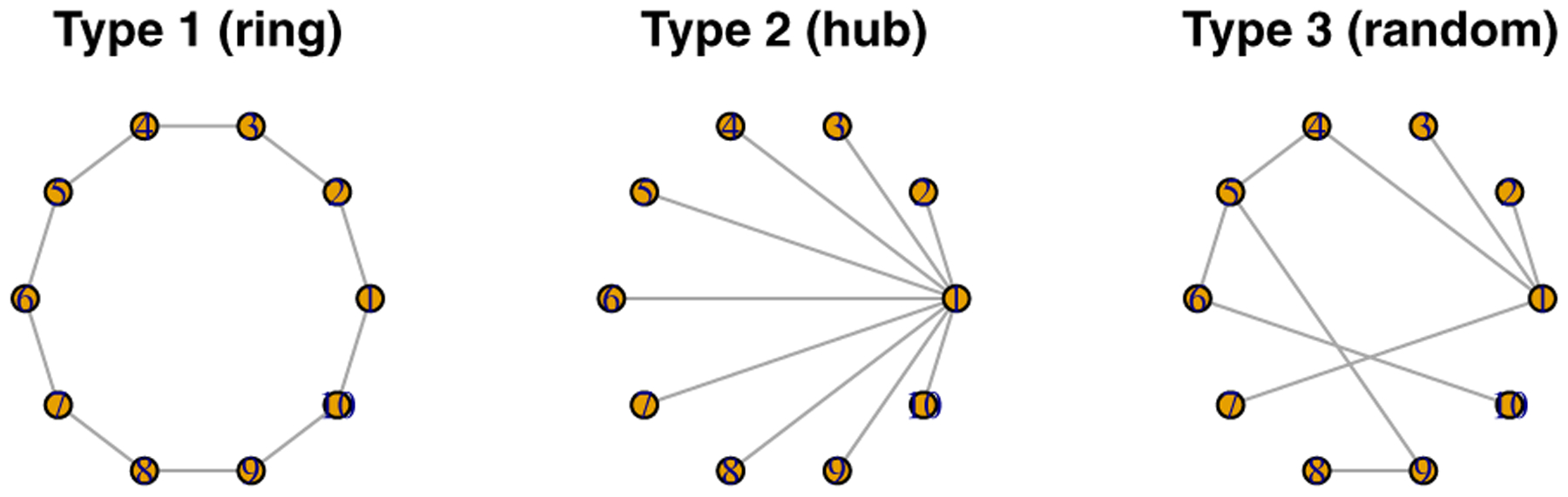
Three types of graph structure for features.

1. Set ${\Omega }_b^m$ to a p_{B ×} p_B zero matrix.

2. Depending on scenarios, generate the lower triangular nonzero elements specified below as $\mathcal{U}\left(-1.5,-0.5\right)$.

   • Scenario 1 (ring type): ${\left[{\mathit{\text{Ω}}}_b^m\right]}_{p_B,1}$ and ${\left[{\mathit{\text{Ω}}}_b^m\right]}_{k,k-1}$ for k > 1 are nonzero.
   • Scenario 2 (hub type): ${\left[{\mathit{\text{Ω}}}_b^m\right]}_{k1}$ for k > 1 are nonzero.
   • Scenario 3 (random type): Each ${\left[{\mathit{\text{Ω}}}_b^m\right]}_{j,k}$ (j > k) is nonzero with probability 3/p_B.

3. ${\Omega }_b^m\leftarrow {\mathit{\text{Ω}}}_b^m+{\mathit{\text{Ω}}}_b^{mT}$.

4. ${\left[{\mathit{\text{Ω}}}_b^m\right]}_{jj}\leftarrow 0.5-{\sum }_{k=1}^{p_B}{\left[{\mathit{\text{Ω}}}_b^m\right]}_{jk}$.

5. Normalize ${\mathit{\text{Ω}}}_b^m$ such that the diagonal elements of its inverse matrix become 1.

The true regression coefficients β^m is given by

$${\mathit{\beta }}^m={\left[\begin{array}{ccccc}{\mathit{\alpha }}^T{\Omega }_1^m& {\mathit{\alpha }}^T{\Omega }_2^m& 0& \cdots & \mathbf{0}\end{array}\right]}^T,$$

where α = [1 0.3 … 0.3]^T. To create heterogeneity, the second block of features is set to have no influence on the outcome variable with probability 1/M. That is, we have

$${\mathit{\beta }}^m={\left[\begin{array}{ccccc}{\mathit{\alpha }}^T{\Omega }_1^m& 0& 0& \cdots & \mathbf{0}\end{array}\right]}^T\mathrm{w}.\text{p}.1/M.$$

For each scenario, each row of X^m is independently sampled from $\mathcal{N}\left(0,{\left({\Omega }^m\right)}^{-1}\right)$. Then, the responses are generated by a linear model as follows.

$$y^m=X^m{\mathit{\beta }}^m+e^m,$$

where $e^m~\mathcal{N}\left(0,{\sigma }^{2}I\right)$.We generate a total of N = nM observations with each data set assigned n samples.

We consider M = 5 data sets with p = 100 features (B = 10, p_B = 10). The error variance is σ² = 1. The training sample size is n = 200, the validation sample size is n_v = 200, and the testing sample size is n_t = 1000. Every method is fitted for a total of 100 replicates and tuned by the validation method. Table 1 reports the simulation results evaluated by the mean squared prediction error (MSE), the average L₂ distance between the estimated coefficients and the true coefficients, the false positive rates (FPR), and the false negative rates (FNR).

Table 1:

Simulation results.

Type	Method	$\mathcal{G}$	Scenario 1				Scenario 2				Scenario 3
			MSE	L2	FNR	FNR	MSE	L2	FNR	FNR	MSE	L2	FNR	FNR
	Lasso		1.252	1.458	0.301	0.246	1.195	1.532	0.195	0.602	1.251	1.477	0.307	0.288
FHT	Enet		1.252	1.458	0.301	0.246	1.195	1.532	0.195	0.602	1.251	1.477	0.307	0.288
	SRIG	Y	1.147	1.002	0.127	0.114	1.136	1.167	0.079	0.000	1.168	1.145	0.194	0.078
	gLasso		1.178	1.252	0.595	0.028	1.162	1.392	0.483	0.222	1.178	1.257	0.598	0.080
	L2 gMCP		1.170	1.219	0.024	0.378	1.186	1.344	0.027	0.705	1.155	1.124	0.033	0.358
	GRIA-Lasso	Y	1.095	0.819	0.161	0.017	1.130	1.044	0.159	0.000	1.107	0.914	0.248	0.015
	GRIA-MCP	Y	1.119	0.980	0.041	0.069	1.132	1.006	0.054	0.000	1.124	1.012	0.070	0.051
	sgLasso		1.276	1.737	0.111	0.206	1.186	1.629	0.115	0.656	1.278	1.762	0.117	0.326
IHT	L1 gMCP		1.191	1.253	0.035	0.382	1.196	1.398	0.008	0.770	1.191	1.252	0.034	0.416
	sGRIA-Lasso	Y	1.106	0.845	0.164	0.025	1.129	1.029	0.159	0.000	1.113	0.937	0.229	0.022
	sGRIA-MCP	Y	1.144	1.078	0.028	0.120	1.134	1.010	0.037	0.002	1.142	1.078	0.044	0.098

FHT; fully heterogeneous models, IHM; integrative homogeneity models, IHT; integrative heterogeneity models, $\mathcal{G}$; Y indicates the method incorporates graph information, MSE; mean squared prediction error, L₂; average L₂ distance between estimated coefficients and true coefficients, FPR; false positive rates, FNR; false negative rates.

First, note that the integrative homogeneity models (IHM) give better performance than the fully heterogeneous methods (FHT), as IHMs are able to integrate the sparsity structure of the coefficients. Considering the fact that the simulated coefficients possess heterogeneity in their sparsity structure, it is somewhat surprising to see IHMs are also better than the integrative heterogeneity models (IHT), but it is because they lose the weak important signals as confirmed by the increased false negative rates.

In the mean time, our proposed methods, which incorporate the graphical information, clearly show improved performance. Not only our two IHM versions (GRIA-Lasso, GRIA-MCP) show the best performance among all competitors, but also we can see our two IHT versions (sGRIA-Lasso, sGRIA-MCP) lose some weak signals, but much less than the existing IHT methods (sgLasso, L₁ gMCP) do. This demonstrates the advantages of incorporating network information into integrative analysis.

6. Application

Alzheimer’s disease (AD) is a cause of dementia which takes into account a majority of dementia cases. AD patients are seriously interfered by loss of memory or other cognitive abilities in their daily lives. The Alzheimer’s disease neuroimaging initiative (ADNI) is a large scale multisite longitudinal study where researchers at 63 sites track the progression of AD in the human brain through the process of normal aging, early mild cognitive impairment (EMCI), and late mild cognitive impairment (LMCI) to dementia or AD. The goal of the study is to validate diagnostic and prognostic biomarkers that can predict the progress of AD.

In our study, we investigate the association of patients’ gene expression levels with their AD progression status. The data set has been downloaded from the ADNI database (www.loni.ucla.edu/ADNI). We treat the fluorodeoxyglucose positron emission tomography (FDG-PET) averaged over the regions of interest (ROI) as the response variable, which measures cell metabolism. The cells affected by AD tend to show reduced metabolism. We suppose the association of FDG with gene expression levels may change as AD makes progress. Therefore, we divide the total of 675 subjects into three groups depending on their baseline disease status. The groups of MCI (EMCI+LMCI), AD, and CN (cognitively normal) are composed of 402, 44, and 229 samples, respectively.

The samples in each group are randomly shuffled and divided into a training set (50%), a validation set (25%), and a testing set (25%). For each shuffle, we fit with our method and all other methods considered in Section 5 plus some fully homogeneous models to check the heterogeneity of the data sets, and then record the prediction errors for the testing samples. This procedure is repeated for 100 random shuffles of the data and the average squared prediction errors are reported in Table 2.

Table 2:

Average prediction errors for ADNI data set.

Type	Method	$\mathcal{G}$	M = 2		M = 3
			MCI	AD	MCI	AD	CN
	Lasso		0.897	0.958	0.931	1.022	0.989
FHM	Enet		0.915	0.938	0.886	1.011	0.943
	SRIG	Y	0.882	0.935	0.864	1.033	0.933
	Lasso		0.917	0.995	0.917	0.995	0.978
FHT	Enet		0.874	0.919	0.874	0.919	0.939
	SRIG	Y	0.860	0.905	0.860	0.905	0.936
	gLasso		0.955	0.952	0.939	0.955	0.985
IHM	L2 gMCP		0.928	0.964	0.922	0.962	0.981
	GRIA-Lasso	Y	0.871	0.911	0.877	0.916	0.930
	GRIA-MCP	Y	0.870	0.900	0.868	0.908	0.916
	sgLasso		0.951	0.963	0.933	0.947	0.986
IHT	L1 gMCP		0.941	0.969	0.962	0.934	0.966
	sGRIA-Lasso	Y	0.857	0.916	0.863	0.920	0.928
	sGRIA-MCP	Y	0.869	0.898	0.865	0.897	0.918

FHM; fully homogeneous models, FHT; fully heterogeneous models, IHM; integrative homogeneity models, IHT; integrative heterogeneity models, $\mathcal{G}$; Y indicates the method incorporates graph information.

First, we only consider two data sets MCI and AD (M = 2). Note that no fully homogeneous method is best performing, which strongly suggests that the two groups are indeed heterogeneous. Despite such heterogeneity, our methods show the close to best performance. The existing integrative analysis approaches, which do not incorporate network information, seem to have difficulty integrating information from different data sets.

Next, we add all groups to the analysis (M = 3). The fully homogeneous methods encounter greater difficulty particularly in predicting the AD group, confirming the increased heterogeneity among the three data sets. The existing integrative analysis approaches show better performance for MCI and AD, but their performance is still not comparable to our methods. In contrast, our methods predict the CN group very well and more importantly still predict the other groups reasonably well without being interfered by the added group, demonstrating the benefits of graphical integrative analysis.

Surprisingly, the fully heterogeneous SRIG also shows the close to best performance for MCI and AD groups. This again advocates incorporating network information. But, it performs slightly worse in predicting CN group than GRIAs.

7. Discussion

We have proposed a novel integrative analysis method, called GRIA, which can incorporate the graphical structure of features. GRIA is very scalable and has been shown to outperform existing integrative analysis approaches through a simulation study and a real data analysis.

Note that incorporating the graphical information can be misleading in some sense. First, the graphical information is still growing and not complete yet. Second, when screening applied, the graphical structure among selected features changes. As a remedy, one can think of a hybrid approach, where we combine the edges detected from the data with the known network information, and use it as our graph knowledge for further analysis. This deserves a future research.

References

- [1].BECK A AND TEBOULLE M, A fast iterative shrinkage-thresholding algorithm for linear inverse problems, SIAM Journal on Imaging Sciences, 2 (2009), pp. 183–202. [Google Scholar]
- [2].CHANG C, KUNDU S, AND LONG Q, Scalable bayesian variable selection for structured high-dimensional data, Biometrics, 74 (2018), pp. 1372–1382. [DOI] [PMC free article] [PubMed] [Google Scholar]
- [3].GONG P, ZHANG C, LU Z, HUANG JZ, AND Ye J, A general iterative shrinkage and thresholding algorithm for non-convex regularized optimization problems, in Proceedings of the 30th International Conference on International Conference on Machine Learning - Volume 28, ICML’13, JMLR.org, 2013, pp. II-37–II-45. [PMC free article] [PubMed] [Google Scholar]
- [4].HUANG Y, ZHANG Q, ZHANG S, HUANG J, AND MA S, Promoting similarity of sparsity structures in integrative analysis with penalization, Journal of the American Statistical Association, 112 (2017), pp. 342–350. [DOI] [PMC free article] [PubMed] [Google Scholar]
- [5].JACOB L, OBOZINSKI G, AND VERT J-P, Group lasso with overlap and graph lasso, in Proceedings of the 26th Annual International Conference on Machine Learning, ICML ‘09, New York, NY, USA, 2009, ACM, pp. 433–440. [Google Scholar]
- [6].KANEHISA M, FURUMICHI M, TANABE M, SATO Y, AND MORISHIMA K, Kegg: new perspectives on genomes, pathways, diseases and drugs, Nucleic Acids Research, 45 (2017), pp. D353–D361. [DOI] [PMC free article] [PubMed] [Google Scholar]
- [7].LI C AND LI H, Network-constrained regularization and variable selection for analysis of genomic data, Bioinformatics, 24 (2008), pp. 1175–1182. [DOI] [PubMed] [Google Scholar]
- [8].LI F AND ZHANG NR, Bayesian Variable Selection in Structured High-Dimensional Covariate Spaces with Applications in Genomics, Journal of the American Statistical Association, 105 (2010), pp. 1202–1214. [Google Scholar]
- [9].LI Q, WANG S, HUANG C-C, YU M, AND SHAO J, Meta-analysis based variable selection for gene expression data, Biometrics, 70 (2014), pp. 872–880. [DOI] [PubMed] [Google Scholar]
- [10].LI Z, CHANG C, KUNDU S, AND LONG Q, Bayesian generalized biclustering analysis via adaptive structured shrinkage, Biostatistics, (2018). kxy081. [DOI] [PMC free article] [PubMed] [Google Scholar]
- [11].LIU J, HUANG J, AND MA S, Incorporating network structure in integrative analysis of cancer prognosis data, Genetic Epidemiology, 37 (2013), pp. 173–183. [DOI] [PMC free article] [PubMed] [Google Scholar]
- [12].Liu j., Huang j., Zhang y., Lan q., Rothman n., Zheng t., and Ma s., Integrative analysis of prognosis data on multiple cancer subtypes, Biometrics, 70 (2014), pp. 480–488. [DOI] [PMC free article] [PubMed] [Google Scholar]
- [13].LIU J, MA S, AND HUANG J, Integrative analysis of cancer diagnosis studies with composite penalization, Scandinavian Journal of Statistics, 41 (2014), pp. 87–103. [DOI] [PMC free article] [PubMed] [Google Scholar]
- [14].MA S, HUANG J, AND SONG X, Integrative analysis and variable selection with multiple high-dimensional data sets, Biostatistics, 12 (2011), pp. 763–775. [DOI] [PMC free article] [PubMed] [Google Scholar]
- [15].MIN EJ, CHANG C, AND LONG Q, Generalized bayesian factor analysis for integrative clustering with applications to multi-omics data, in 2018 IEEE 5th International Conference on Data Science and Advanced Analytics (DSAA), October 2018, pp. 109–119. [DOI] [PMC free article] [PubMed] [Google Scholar]
- [16].PAN W, XIE B, AND SHEN X, Incorporating predictor network in penalized regression with application to microarray data, Biometrics, 66 (2010), pp. 474–484. [DOI] [PMC free article] [PubMed] [Google Scholar]
- [17].SIMON N, FRIEDMAN J, HASTIE T, AND TIBSHIRANI R, A sparse-group lasso, Journal of Computational and Graphical Statistics, 22 (2013), pp. 231–245. [Google Scholar]
- [18].STINGO FC, CHEN YA, TADESSE MG, AND VANNUCCI M, Incorporating Biological Information into Linear Models: A Bayesian Approach to the Selection of Pathways and Genes, Annals of Applied Statistics, 5 (2011), pp. 1978–2002. [DOI] [PMC free article] [PubMed] [Google Scholar]
- [19].TIBSHIRANI R, Regression shrinkage and selection via the lasso, Journal of the Royal Statistical Society: Series B (Methodological), 58 (1996), pp. 267–288. [Google Scholar]
- [20].YU G AND LIU Y, Sparse regression incorporating graphical structure among predictors, Journal of the American Statistical Association, 111 (2016), pp. 707–720. [DOI] [PMC free article] [PubMed] [Google Scholar]
- [21].YUAN M AND LIN Y, Model selection and estimation in regression with grouped variables, Journal of the Royal Statistical Society: Series B (Statistical Methodology), 68 (2006), pp. 49–67. [Google Scholar]
- [22].ZHANG C-H, Nearly unbiased variable selection under minimax concave penalty, Ann. Statist, 38 (2010), pp. 894–942. [Google Scholar]
- [23].ZHAO Q, SHI X, HUANG J, LIU J, LI Y, AND MA S, Integrative analysis of ‘-omics’ data using penalty functions, Wiley Interdisciplinary Reviews: Computational Statistics, 7 (2015), pp. 99–108. [DOI] [PMC free article] [PubMed] [Google Scholar]
- [24].ZOU H AND HASTIE T, Regularization and variable selection via the elastic net, Journal of the Royal Statistical Society: Series B (Statistical Methodology), 67 (2005), pp. 301–320. [Google Scholar]