Abstract
When a scanner is installed and begins to be used operationally, its actual performance may deviate somewhat from the predictions made at the design stage. Thus it is recommended that routine quality assurance (QA) measurements be used to provide an operational understanding of scanning properties. While QA data are primarily used to evaluate sensitivity and bias patterns, there is a possibility to also make use of such data sets for a more refined understanding of the 3-D scanning properties. Building on some recent work on analysis of the distributional characteristics of iteratively reconstructed PET data, we construct an auto-regression model for analysis of the 3-D spatial auto-covariance structure of iteratively reconstructed data, after normalization. Appropriate likelihood-based statistical techniques for estimation of the auto-regression model coefficients are described. The fitted model leads to a simple process for approximate simulation of scanner performance—one that is readily implemented in an script. The analysis provides a practical mechanism for evaluating the operational error characteristics of iteratively reconstructed PET images. Simulation studies are used for validation. The approach is illustrated on QA data from an operational clinical scanner and numerical phantom data. We also demonstrate the potential for use of these techniques, as a form of model-based bootstrapping, to provide assessments of measurement uncertainties in variables derived from clinical FDG-PET scans. This is illustrated using data from a clinical scan in a lung cancer patient, after a 3-minute acquisition has been re-binned into three consecutive 1-minute time-frames. An uncertainty measure for the tumor SUVmax value is obtained. The methodology is seen to be practical and could be a useful support for quantitative decision making based on PET data.
Keywords: Quality assurance, Simulation, Spatial autocorrelation, PET, Iterative EM reconstruction, Gamma distribution, Conditional likelihood, Model-based bootstrap, Standard errors
I. INTRODUCTION
IN many institutions, positron emission tomography (PET) imaging plays a key role in the routine clinical management of cancer patients, as well as with some important cardiac and neurologic conditions. With the growing reliance on PET imaging information for clinical decision making, there is an ongoing need to have more detailed quantitative understanding of the operational characteristics of reconstructed PET images. This can facilitate consistent clinical decision-making based on the PET at a given institution and may also enable the conduct of multi-institution clinical trials involving PET imaging biomarkers [22]. Going back to the 1980s [13], routine quality assurance (QA) is a well established part of nuclear medicine practice and in particular of PET. The standard approach to QA with PET is to image a known source—physical phantom scans—and use the results to assess bias and sensitivity patterns. Sensitivity plays a key role in understanding local variance characteristics. There is a significant literature on methods for assessment of the statistical variation of PET data. Most of this has focused on approximating standard errors for regional averages of reconstructed data using a combination of analytic and empirical formulae [1, 2, 5, 11, 12, 15, 19, 24, 27]. The potential use of bootstrap methodologies in this context is appealing but for iterative reconstructions the computation requirements of the approach have limited its use in an operational settings, especially for dynamic studies.
Recently we presented a novel approach to the analysis of bias and sensitivity in a PET scanner based on QA data derived from a uniform source phantom [18]. Results showed that iteratively reconstructed PET image data were well described by Gamma statistics. Within the Gamma framework, characterization of bias and sensitivity can be efficiently carried out in terms of a multiplicative model analysis [18]. As part of our study it was found that, through a standard probability transform which adjusts for bias and sensitivity, raw reconstructed PET image data can be converted into a normalized Gaussian scale. This analysis methodology was implemented in an [25] script.
The goal of the present work is to extend the previous analysis in order to obtain a practical representation of the full covariance characteristics of iteratively reconstructed PET data. We propose spatial autoregressive (SAR) models for representation of the 3-D spatial correlation structure of appropriately normalized data. The SAR approach involves relating the behavior of each voxel to the behavior on its neighbors. The first and second order neighbors are considered. Estimation of the SAR model cannot be accomplished by straightforward adaptation of the Yule-Walker process used for estimation of 1-D AR models [3]. Indeed such an approach can sometimes be inconsistent. The phenomenon is illustrated in section II-B. To resolve this estimation problem, we adapt a general likelihood based methodology for SAR model estimation.
The implementation makes use of the fast Fourier transform (FFT). The proposed approach leads to a consistent estimation process which provides a simple and practical approach for data analysis. Combining our previous work with this new development leads to a simplified approach to simulating PET images with noise characteristics that are matched to the operational scanner. Thus routine QA data can provide a mechanism for empirically representing the uncertainties in PET scan measurements.
The basic theory and methodology is developed in section II. Studies with real and simulated data are described in section III. Included in our analysis are data from a clinical PET-FDG scan. This is used to demonstrate the potential of the methodology to create practical assessments of uncertainty, via model-based bootstrapping [7]. Section IV presents the results for both EM reconstructed data and simulated data. The paper concludes with discussion.
II. Methodological Development
The data structure arising from a physical phantom study is a set of reconstructed PET measurements corresponding to a collection of N voxels consisting of I1 × I2 phantom-voxels recorded on each of I3 transverse slices in the field of view of the scanner. These data correspond to a particular acquisition time-frame during which the phantom is measured in the scanner field of view. In a dynamic PET study there will be multiple time-frames, but, as data from distinct time-frames can be considered to arise as a processed version of a thinned 4-D Poisson process, these can be considered as independent of each other. Our focus is on PET data that has been iteratively reconstructed using some variation on the EM algorithm [26].
A. Spatial Autoregressive Model
In previous work, we demonstrated that iteratively reconstructed PET data could be represented using the Gamma distribution [18]. So
where (n1, n2) are transverse plane co-ordinates and n3 indexes the slice. μ(n) is the activity of the target source activity per unit mass (scaled by dose), ϕ(n) models scanner and object-specific factors (most notably attenuation) that contribute to extra-Poisson variation, τ is proportional to the injected dose per unit mass of the object. The Gamma model allows us to normalize PET data to a Gaussian scale via the probability transform [18]:
| (1) |
where is the Gamma cumulative distribution function with mean and variance . Both and can be estimated from phantom data measurements [18]. Φ is the standard normal cumulative distribution function.
Here we propose to analyze the 3-D covariance of the normalized data using spatial autoregressive (SAR) models. A SAR model specifies a linear relation between a collection of appropriately defined neighbors
| (2) |
where u(n) = u(n1, n2, n3) and the summation is made over a set of negative and positive indices, k = (k1, k2, k3), such that voxels (n − k) belong to an appropriate neighborhood of the voxel n—this will be detailed below. ϵ(n) is a Gaussian white noise process with variance σ2. θk is the coefficient of the corresponding neighbor (n − k). By introducing a linear difference operator the model can be expressed as
| (3) |
where u(n) and ϵ(n) represent the data and the innovation white noise process evaluated at the n’th voxel and Bku(n) = u(n − k) = u(n1 − k1, n2 − k2, n3 − k3). In practice only a small number of θk coefficients are non-zero. A first order model will only involve terms where all components of k are zero, except one being 1 in absolute value; an s’th order model only has non-zero terms for k = (k1, k2, k3)’s in which |k1| + |k2| + |k3| ≤ s. Models of order 2 seem adequate according to the empirical analysis of phantom data and simulated data in IV. SAR models are generalizations of simple auto-regressive (AR) models used in classical time series analysis [3, 4]. See Yao and Brockwell [29] for discussion of spatial generalizations of classical ARMA time series models. SARs have been proposed for analysis of spatial processes [9, 16, 21, 28], but to our knowledge, they have not been applied to nuclear medicine imaging data. The SAR models used in spatial statistics are sometimes specified so that the θ-coefficients are known up to some scale factor determined from available data [8]. In our case we are interested in SAR models in which the full set of non-zero θ-coefficients must be estimated from the available data.
B. Estimation of SAR Model Coefficients
While the method of least squares is a standard (and asymptotically optimal) approach for estimation of familiar AR model coefficients [3, 4], it runs into problems for more general auto-regressions. This was highlighted by Whittle [28]. To illustrate this, consider a SAR model in time
for t = 0, ±1, ±2, ..., T and ϵt white noise, where yt±1, yt±2 are the 1- and 2-order neighbors of yt. The least squares estimates of θ = (θ1, θ2) minimize
where with B is the backshift and is the set of data indices and are the indices of unobserved y-values which are needed in order to reconstruct the innovations ϵ(t) at the sampled points. For large T, the impact of unobserved data is negligible. Least squares coefficients satisfy the normal equations. Derived from the Yule-Walker equations for an AR(2) process , where γl is the auto-covariance function of yt, the AR parameters are determined by the first p + 1 elements ρ(l) of the auto-correlation function . In the present situation for large T, these coefficients (denoted as ) for k = −2, −1, 1, 2 are identified by
| (4) |
where ρl is the auto-correlation at lag l for l = 1, 2, 3, 4. It is not hard to find a situation where the estimates are inconsistent. For example, if θ = (0.30, 0.02) then . In light of this, least-squares auto-regression may not be relied on for estimation of SAR models parameters.
Likelihood-based approaches to the estimation of SAR and ARMA models are well established and have the familiar behavior of regular maximum likelihood procedures [16, 29]. In the case of an SAR it is well known, see e.g. Mohalp [16], that the appropriate (conditional) likelihood-based objective function can be expressed as
| (5) |
where N is the number of voxels in , λ = (λ1, λ2, λ3) and is the 3-d spectral density of the SAR process., with , is the 3-D discrete Fourier transform of the SAR coefficients. Differentiating equation (5) with respect to θ and setting the derivative to zero we obtain a pseudo-linear (score) equation for the unknown components of θ
| (6) |
where indexes the relevant components of non-zero θ’s, is the spectral density. Using Parseval’s relation, the above equation can be expressed as a requirement that the maximum likelihood estimators ensure that select sample auto-covariances, at lags corresponding to the non-zero θ, match the model-predicted covariances
| (7) |
for . Here is a sample estimate of the auto-covariance and the inverse Fourier transform of the spectral density fθ(λ) gives the 3-D model auto-covariance,. Equation (7) might be compared to the score equation that would arise in the minimization of the non-linear least-squares objective function
| (8) |
where , wm is the number of l′ − l such that |l′ − l| = m and and . Estimation of θ can be expected to produce estimates of the auto-covariance that are in close agreement with sample auto-covariance values.
C. Neighborhood Structure
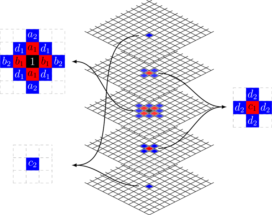
Model (2) is based on specification of the neighborhood structure of each voxel. Image data has a regular structure and there are several intuitive strategies for defining the neighborhood structure of a voxel [6]. We define the s’th order neighborhood of (i, j, k) as
The first (s = 1) and second (s = 2) neighborhood structures are sketched in Fig. 1. The first order neighborhood is also known as the 3-D Rook neighborhood [30].
Fig. 1.
Diagram of first (red) and second (blue) order neighbors for a selected voxel (black) with a set of coefficients for each neighbor.
D. ACF Computation
This section describes a fast and simple computation of ACF. The hyper-rectangular volume of the normalized data—u(n) can be processed using the 3-D FFT to obtain the periodogram, fN(λ). The inverse FFT of the periodogram provides a set of sample auto-covariances cN(m). For a specified θ we sample at the same discrete Fourier frequencies as the periodogram and apply the inverse FFT, followed by normalization to ensure c(0|θ) = cN(0), this provides the model auto-covariances, c(m|θ). These are used to evaluate (8). Note the auto-correlations of the data and the model are obtained as
E. Simulation of PET Data
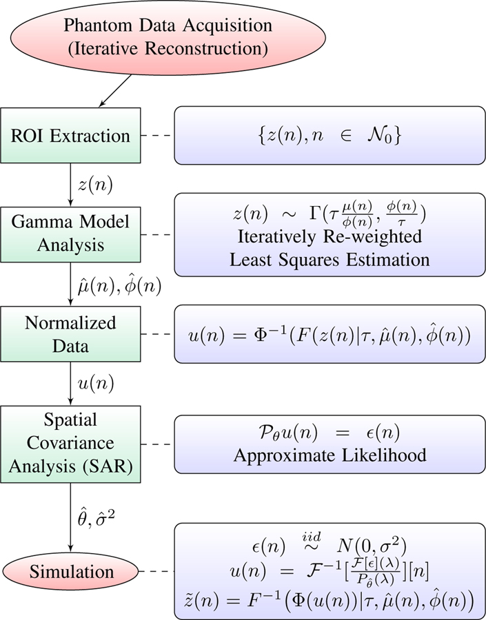
The Cramer representation theorem, see e.g. Mohalp [16], provides a mechanism to simulate normalized PET data and by inverting the Gamma model probability transform in equation (1), these data can be converted into simulated PET image values for z(n). The process is as follows: First generate ϵ(n) as an iid N (0, σ2) process; transform ϵ(n) using the FFT and scale by the Pθ(λ). Next apply the inverse FFT to generate the normalized data u(n). These steps are summarized by the formula.
where represents the FFT. Finally simulated PET values are obtained as
The analysis method and simulation step is summarized graphically in Fig. 2.
Fig. 2.
Graphical representation of the PET analysis and simulation process.
III. Experimental Methods
A. Normalized Physical Phantom Data Analysis
Routine quality assurance monitoring of the performance of installed scanners involves a range of phantom tests matched to operational clinical practice. We consider the data of this type collected at a PET imaging facility at a local hospital— the Cork University Hospital (CUH). The scanner is a GE Discovery VCT PET/CT and used clinically for imaging of cancer patients. The reconstruction process used is an OSEM technique with 3 iterations and 28 subsets. This is approximately equivalent to 120 iterations of a standard EM algorithm [17]. In our study, the scanning procedure was in line with a standard dynamic PET-FDG brain imaging protocol developed by the American College of Radiology Imaging Network (ACRIN) [22]. The cylindrical phantom is 189 mm in length and 195 mm in diameter, filled with a mixed solution of F-18 radiotracer and water and placed centrally in the field of view (FOV). Routine clinical image reconstruction is performed with the iterative OSEM reconstruction technique (3D-IR). A dynamic sequence of 45 time-frames is acquired for 55 minutes. For each time-frame, the reconstructed image has 128×128 pixels in 47 slices, with pixel size of 5.46875× 5.46875 mm2 and slice thickness of 3.27 mm. Region of interest (ROI) data for the interior cross-sectional circular volume of the phantom, acquired for each axial slice (except two extreme slices), k, and for each time-frame, t, are available for analysis. The data for the set of all K slices and T time-frames structured as {zikt, i = 1, 2, ..., N, k = 1, 2, ..., K, t = 1, 2, ..., T}. In general, PET images from different time-frames are independent, here we just focus on the data from a single time-frame—the t = 24 frame.
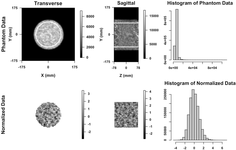
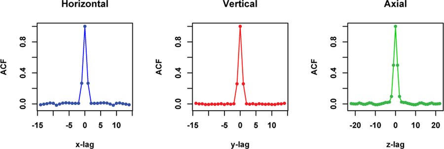
Based our previous work [18], measurements have been normalized based on the multiplicative Gamma model. The normalized data are well described by the Gaussian distribution (c.f. Fig. 3). Based on the analysis of 3-D autocorrelation of the phantom data (Fig. 4), there is little rotational variation in row and column directions within each slice. Hence we consider all voxels within the ROI where both 1- and 2-order neighbors are available. Reasonably assuming that the data on each direction (row, column and axial) are symmetric, we denote the regression coefficients as shown in Fig. 1. We apply the methodology developed in the previous section to fit to SAR models to the normalized data. The order of neighborhood, s, is selected based on the significance of regression coefficients and diagnostic analysis of residuals—primarily the residual auto-correlation characteristic [3].
Fig. 3.
Top: The transverse and sagittal image of 3-D dynamic PET study on a cylindrical phantom using iterative (3D-IR) reconstructed methods (24th time frame of slice 23). The ROI data within white outline are used in analysis. On the right is the histogram of the data generated from ROIs. Bottom: Images and histogram of the probability transformed/normalized data generated by the previous study.
Fig. 4.
The 1-D horizontal, vertical and axial profiles through the center of the 3-D ACF image of the ROI data shown in the top of Fig. 3.
B. SAR Model Simulation
To illustrate the performance of the proposed method in estimating SAR model coefficients, we simulate 3-D data according to the following model
for and θk matched to typical values estimated from the CUH phantom. Mean squared errors (MSE) for the θ parameter estimation, defined as where Nθ is the number of the θ parameters, are evaluated as function of ROI size for the noise level matched to the one in the CUH Phantom data.
C. Numerical Phantom Simulation
The uniform elliptical phantom as well as two versions, a symmetric and non-symmetric form, of the 2-D VSK phantom [26] were used. A sinogram source g was evaluated using a simple analytic Radon projection. Sinograms generated from the VSK and uniform phantom were attenuated using the same attenuation matrix that assumed uniform density in the phantom region. Poisson data in the sinogram domain were simulated in [25] using the function rpois. Data were reconstructed using the Expectation-Maximization (EM) algorithm. The EM algorithm, initialized with the true uniform image, is iterated 200 times. For each count rate, 200 replicate runs were conducted to produce 200 replicate images. At each pixel, 200 replicate values were used to estimate Gamma model parameters and probability transformation [18] was performed on each replicate image. Methods developed in Section II were then used to analyze the 2-D autocorrelation of these normalized image data. To investigate effects of the noise level and smoothing on performance of the proposed ACF method, count rates of 105 and 106 were used in simulation of sinograms. Post-reconstruction smoothing with Full Width Half Maximum (FWHM) of 2, 4, 8 pixels was performed. Using 200 replicates, we can calculate the pixel-wise correlation coefficients of reconstructed image data and compare them to ACFs calculated by the proposed method.
D. Model-Based Bootstrapping of a Lung Tumor SUVmax
We consider data selected from clinical PET-FDG scans of a lung tumor patient acquired over a 15-minute time-period, 60 minutes after tracer injection. The full acquisition consisted of 5 bed-positions, each image for a period of 3 minutes. The 3- minute scan data from the bed-position corresponding to the primary tumor, located in the hilar region of the left lung, was re-binned into three consecutive 1-minute frames and iteratively reconstructed using the standard process—e.g. the same as that used in the physical phantom studies conducted on the same scanner (above). Given the metabolism of FDG, it is reasonable to expect that there will be little or no voxel-level temporal variation in the FDG profile in 3 consecutive minutes 60+ minutes after injection. Thus, we may approximately regard the measurements as rough replicates and proceed to evaluate the voxel-by-voxel mean μx and variance and, based on these, recover corresponding voxel-level Gamma model parameters—μ and ϕ. Given the Gamma model parameters, we use the probability transform and analyze the 3-D auto-covariance with the SAR modelling approach. We then apply the scheme in section II-E, see schematic in Fig. 2, to simulate PET scan data and use those simulations to recover assessments of uncertainty in SUV values. The process is an example of a model-based bootstrapping procedure [7] for assessment of uncertainties (standard errors) in measurements. It is of interest here because direct bootstrapping of raw list-mode data [10] is not practically feasible, for routine application. We apply the approach to develop an approximate standard error for the tumor SUVmax.
IV. Results
We begin by presenting results of analysis of physical phantom data, this is followed by numerical simulation studies including SAR model simulation and VSK and uniform phantom simulation. Finally, we present results of analysis of patient data.
A. Physical Phantom Data
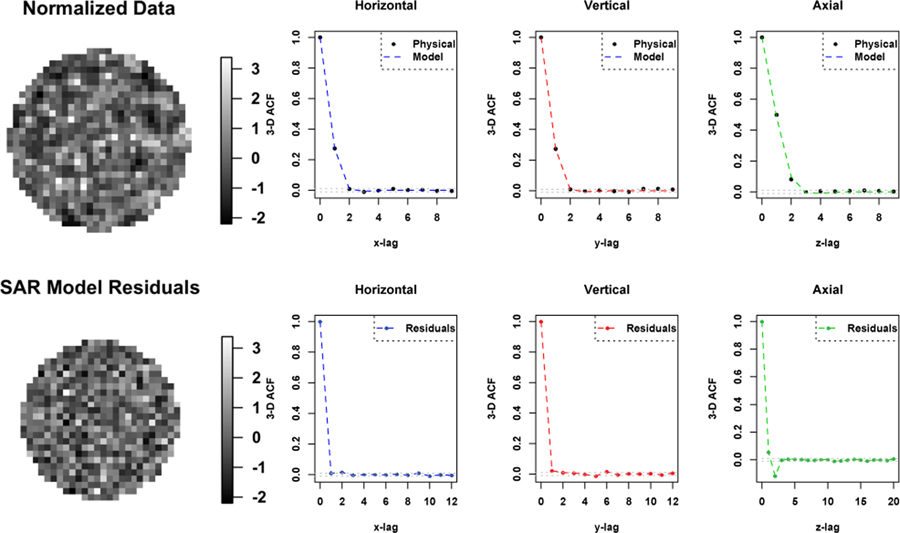
Fig. 3 shows uniform cylindrical phantom data OSEM reconstructed at a PET imaging facility at a local hospital before (the top) and after (the bottom) normalizing based on the Gamma distribution [18]. Histogram at the bottom right indicates that the normalized data can be modelled using the Gaussian distribution. Fig. 4 shows 1-D horizontal, vertical and axial profiles through the center of the 3-D ACF image of the ROI data shown in the top of Fig. 3. We fit a SAR model with the second order neighborhood to the normalized data. The 3-D auto-correlation function (ACF) of the fitted SAR model is plotted as three 1-D profiles in Fig. 5, in comparison with 3-D ACF of the normalized physical phantom data, was calculated as the inverse Fourier transform of the data periodogram as described in II-D. Also shown in Fig. 5 is the 3-D ACF of the fitted SAR model residuals. The 3-D ACF of the normalized data is well described by the model. The model residuals shows no significant autocorrelation present in transaxial directions, but some significant autocorrelation present in axial direction. However, the amplitude of autocorrelation is greatly reduced (in comparison to the normalized data). This may indicate that there is non-stationary axial autocorrelation present in the data. The estimated model coefficients are presented in Table I, where ai, bi, ci are representing the coefficients along vertical, horizontal and axial directions respectively, and di is for diagonal direction as shown in Fig. 1.
Fig. 5.
Top: The transverse image of the normalized physical phantom data and one dimensional profiles of 3-D ACF of the normalized physical phantom data and the fitted SAR model. Bottom: The transverse image and one dimensional profiles of 3-D ACF of the fitted SAR model residuals.
TABLE I.
Non-linear Regression Coefficients
| 0.151 ± 0.005∗ | −0.015 ± 0.002∗ | |||
| 0.149 ± 0.005∗ | −0.014 ± 0.002∗ | |||
| 0.275 ± 0.006∗ | −0.040 ± 0.003∗ | |||
| −0.018 ± 0.003∗ | −0.037 ± 0.003∗ |
denotes significant.
B. SAR Model Simulation
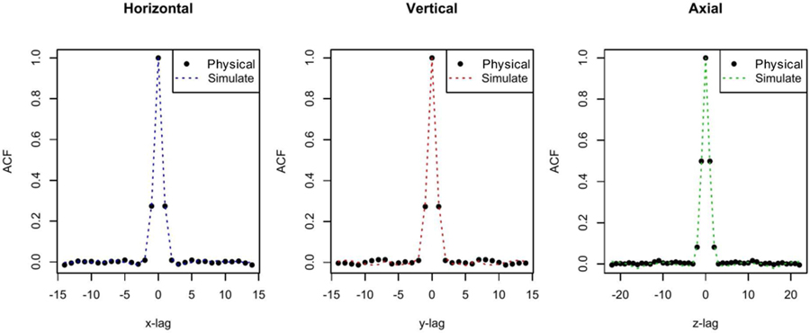
Using the θ parameters estimated from and the same data size as the CUH ROI data for one time frame (sample size N0 = 30 × 30 × 45), Fig. 6 shows that the ACF structure in the CUH ROI data can be well captured and simulated by the simulation model. The R-squared values of the estimated ACFs based on the CUH ROI data and simulated data are 99.86%, 99.51% and 99.56% in the horizontal, vertical and axial direction, respectively. At lag 1 the relative differences between these ACFs are 2.38%, 7.41% and 4.33%, respectively.
Fig. 6.
Comparison of the 3-D ACF of the physical phantom data and the SAR model simulated data in each direction.
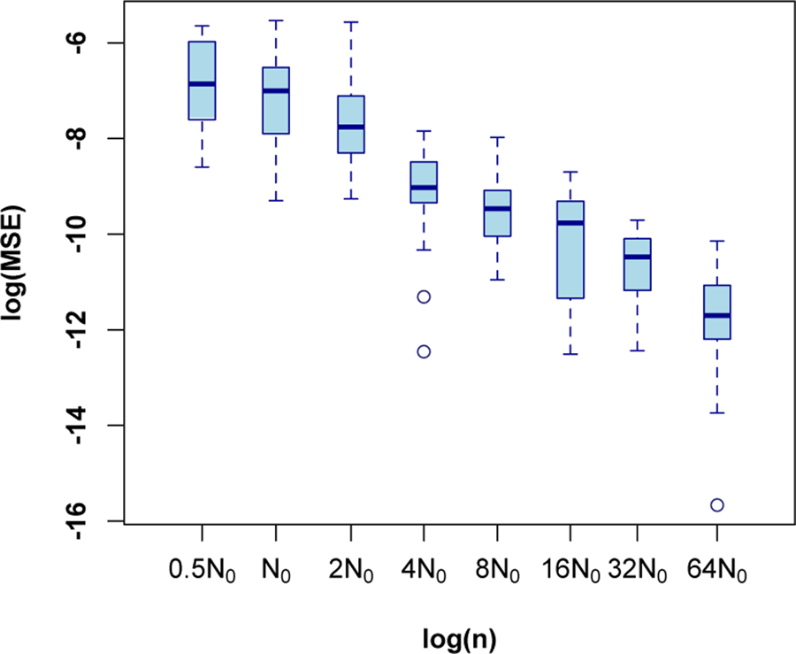
To demonstrate estimation accuracy of the proposed method, data with varying size were generated. The considered data sizes are created by scaling each dimension of the CUH ROI using the same scale factor τ , that is τ N0 for τ = 0.5, 1, 2, 4, . . . , 64. Then the proposed method was applied to the simulated data. This process is repeated 20 times for each data size. Note that the data size in this experiment is referred to the number of pixels used in simulation. Using different data sizes is aimed to investigate convergence of estimators as sample size increases. Fig. 7 shows the log mean square error (MSE) of the θ estimation, defined as , as function of the log sample size τN0. This figure seems to indicate that log MSE decreases linearly in the log sample size, especially after ignoring the first box. The slope-coefficient is estimated as (−1.04 ± 0.06), consistent with asymptotic theory [16].
Fig. 7.
Log mean squared errors (MSE) of the estimated model parameters based on simulation study with different sample sizes (20 repetitions for each size). N0 corresponds to the size of the phantom ROI in the CUH data.
C. Numerical Phantom Simulation
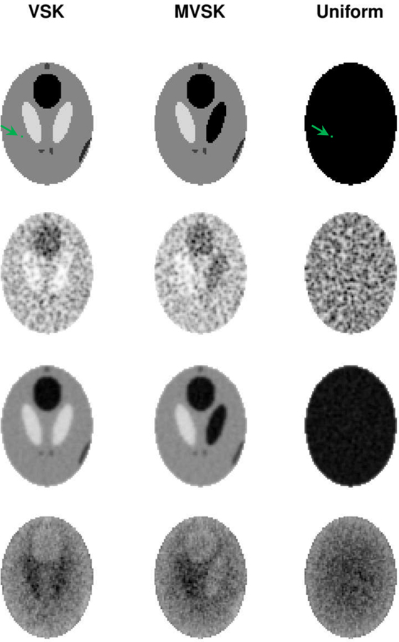
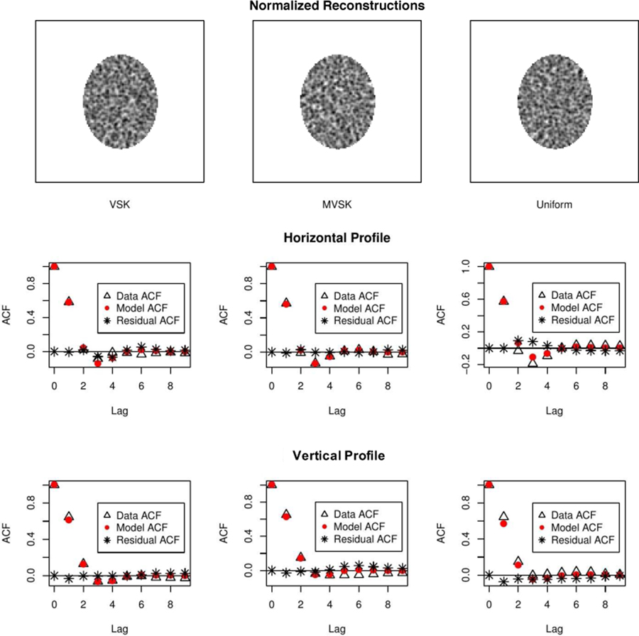
Row 1 of Fig. 8 shows the three phantom images used in the simulation study. Corresponding sample reconstructions are shown in Row 2. Row 3 shows the mean images of 200 replicate reconstructions. ϕ’s computed pixel-wisely by fitting the Gamma distribution to 200 replicate values are shown in Row 4. We applied normalization (1) to each reconstruction using the corresponding ϕ’s and μ’s (means). Samples of normalized reconstruction are shown in Row 1 of Fig. 9. The 1-D horizontal (short-axis of ellipse) and vertical (long-axis of ellipse) profiles through the center of ACF image of normalized reconstruction data are shown in Row 2 & 3. Comparing the ACFs results in Fig. 5 for the cylindrical phantom to the profiles in Fig. 9, we see that while horizontal and vertical profiles are very similar in the cylindrical case, there is evidence of greater persistence in the ACF in the vertical/long-axis profile versus the horizontal/short-axis profiles in the elliptical case. This is consistent with the work of Razifar et. al. [20] who demonstrated a similar effect. Normalized VSK, MVSK and uniform phantom reconstructions exhibit very similar autocorrelation structures, and these auto-correlation structures can be well described by the SAR model. There is no autocorrelation left in the residual image (as shown in Row 2–3 of Fig. 9, residual derviations between the data and SAR model ACFs are all close to zero). To make more reliable comparison between uniform and non-uniform sources, we fitted the SAR model to 100 normalized reconstructions of each phantom. Estimates of the SAR model coefficients are presented in Table II. As shown in the table, there is no significant difference in auto-correlation of normalized reconstructions of different phantoms. This suggests that the autocorrelation pattern may be mostly determined by the attenuation structure and perhaps less influenced by the source configuration within the volume where the source is concentrated.
Fig. 8.
Row 1: The VSK, MVSK and uniform elliptical phantom (from left to right). Row 2: EM reconstructions of the three phantoms; Row 3: The mean images of 200 replicate reconstructions; Row 4: The estimated ϕ(n) of the Gamma model from the 200 replicates. The green colored pixel is an arbitrarily placed reference pixel, which is used to caculate pairwise pixel correlations shown in Fig. 10.
Fig. 9.
Row 1: Normalized reconstruction of the VSK, MVSK and uniform phantoms (from left to right). Row 2 and 3: 1-D horizontal and vertical profiles through the center of the ACF image of normalized reconstruction—data (triangle), the SAR model (red dot) and the residual deviation between data and model(*).
TABLE II.
Fitted SAR Model Coefficients based on normalized reconstruction data
| VSK | MVSK | Uniform | |
|---|---|---|---|
| 0.345 ± 0.038 | 0.346 ± 0.037 | 0.339 ± 0.046 | |
| 0.357 ± 0.035 | 0.355 ± 0.040 | 0.366 ± 0.038 | |
| −0.054 ± 0.014 | −0.056 ± 0.015 | −0.052 ± 0.014 | |
| −0.074 ± 0.013 | −0.074 ± 0.015 | −0.080 ± 0.016 | |
| −0.093 ± 0.029 | −0.093 ± 0.031 | −0.097 ± 0.033 |
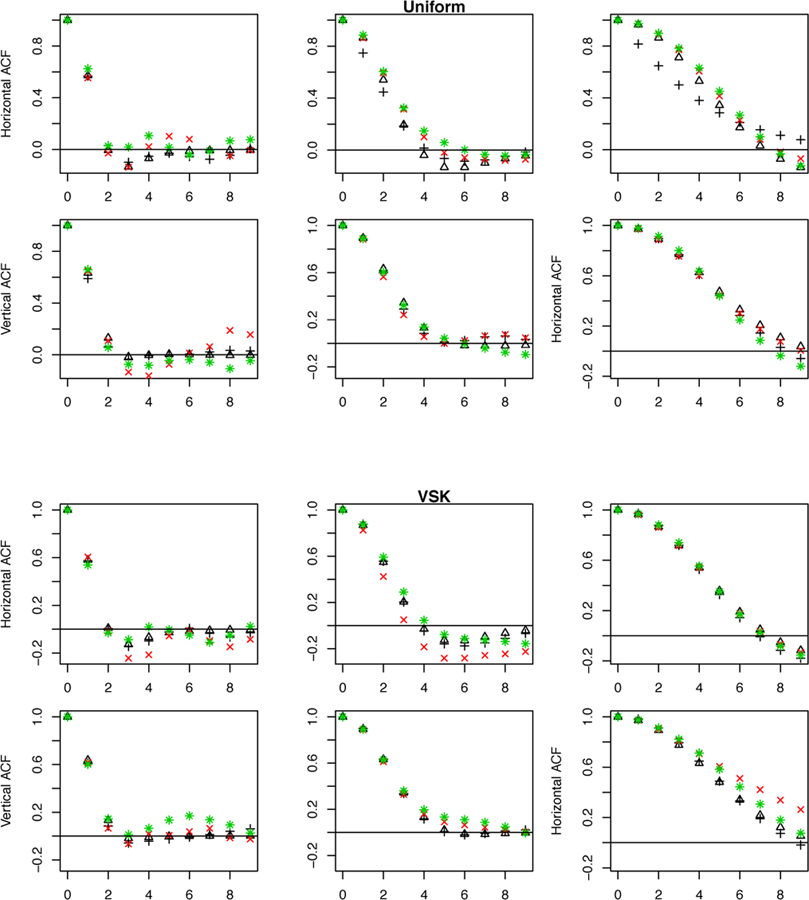
To further validate the ability of the methodology to capture correlation in images with uniform and non-uniform source distributions, Fig. 10 presents the average ACFs of 200 normalized VSK and Uniform reconstructions across a range of count rates (N) and post-reconstruction Gaussian smoothing. Average estimates of SAR model ACF show good agreement with the data. Directly evaluated pairwise pixel-wise correlations evaluated over 200 replicates are also shown. These can be regarded as ground truth—they do not make use of stationarity of the normalized reconstructed data. The results show that correlation is in line with the stationary assumption and can be captured by the ACF of fitted SAR model. Fig. 10 also plots the 1-D profiles of 2-D ACF with and without data transformation. ACFs with and without transformation are very similar. The same patterns are observed in analysis of reconstruction data using count rate of 106 and the MVSK phantom (not shown).
Fig. 10.
Horizontal and vertical profiles of 2-D ACF of Uniform and VSK phantom reconstructions based on a count rate N = 105 with (black triangle) and without probability transformation (black plus), overlaid with correlations of the pixel at the center for 10 lags in different directions (red cross) and the ones of arbitrary pixel closed to edge of the phantom (green star). The pixel is shown on the first row of Fig. 8 as a green dot. From left to right, FWHM of 2, 4 and 8 pixels are used for post-reconstruction smoothing. Calculation is based on 200 replicates for each setting.
D. Model-Based Bootstrapping of a Lung Tumor SUVmax
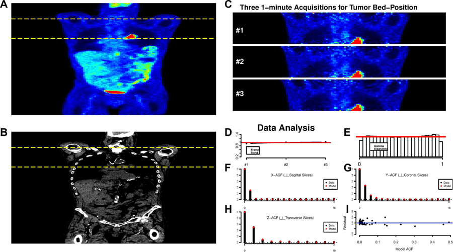
Fig. 11 displays a whole-body FDG-PET/CT study in a lung cancer patient. Both the PET and CT data are presented. The pattern of FDG uptake is very similar on the three consecutive 1-minute frames, see Fig. 11 (C), selected for analysis. We focus analysis on voxels corresponding to the body—thresholding based on the CT and FDG scans is used to eliminate background. The average voxel-level tissue uptake profile, normalized so that , is quite constant across each of the frames. Our analysis adjusts for the very slight increase at the voxel level. Letting zxj be the observed SUV at voxel x and frame j, we model these voxel-level data as
Fig. 11.
A: Whole-body coronal views of the FDG uptake, 60–75 mins post injection. B: The corresponding CT scan. The yellow dashed lines indicate the bed-position corresponding to the lung tumor in the hilar region of the left lung. C: Coronal views of consecutive 1-minute scans obtained from the 3-minute acquisition of raw list-mode data over the tumor bed position. D: Profile of the average uptake profile per voxel as a function of acquisition, constant profile shown in red. E: Histogram of the Gamma transformed voxel level data—the red line shows the reference uniform. F-H: ACF plots of the probability transformed data (black), in 3 co-ordinate directions. The fit of the SAR model is shown in red. I: Deviations between the full 3-ACF and the fitted SAR model ACF.
with γx estimated by the simple average,. Assuming a Gamma model in which ϕx is constant across replicates, we estimate ϕx by the average
An argument could be made for division by 3 instead of 2 in this formula. We have been guided by the principle that, given the estimation of γx, there are at most 2 degrees of freedom associated with the deviations between zxj and . It is important to note that here ϕ, includes the effect of dose. Given that our analysis, see last row of Fig. 8 indicates that ϕ should be very regular, it is appropriate to smooth the raw estimates in order to improve the expected mean squared error of the estimation—we use a simple 3-D Gaussian with FWHM of 2-voxels in x-y direction in transverse planes and also axially. Given estimates of γx and ϕx, a Gamma transformed variable is created, at each voxel and at each replicate value, as
where F is the cumulative Gamma distribution. If the Gamma-model is correct the transformed data should have a uniform distribution.
The data analysis results in Fig. 11 (D–I) show substantial consistency with the Gamma assumption, practically validating our estimation of γx, μj and ϕx. Note we also considered the distribution of the uxj-values within individual replicates and on different axial planes within the tumor-bed. The uniformity check of the Gamma structure was reasonable throughout. Next, the uxj data were transformed into standard Gaussian values, , and the 3-D ACF of the rxj-data evaluated. Using techniques described earlier, a second order SAR model was found to provide a good representation of the 3-D ACF. Fig. 11 (F–H) show the sample ACF and together with the fitted SAR model. The overall fit appears quite satisfactory. It is notable that there is a difference between the range of the ACF in the x and y directions. This is unlike the physical phantom data, where the within transverse planes the ACF in the horizontal(x) and vertical(y) directions matched and is also unlike our numerical simulations where the ACF was slightly more persistent in the long-axis direction. The ACF here is seen to be more persistent perpendicular to coronal planes (the short axis) than in the direction perpendicular to sagittal planes (the long-axis). The effect is consistent across all planes within the tumor bed position.
Given our analysis of the replicates we are in a position to simulate synthetic copies of the patients 3-D SUV scan data. This follows the scheme indicated in section II-E. We begin by simulating three independent 3-D Gaussian processes, ϵxj for j = 1, 2, 3, each with ACF given by the SAR model. As before, this simulation is generated with reliance on the spectral density corresponding to the SAR model and the 3-D FFT. Given ϵxj, SUV values are produced by
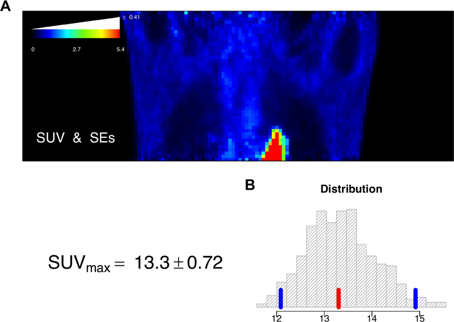
The average of these SUV values over replicates, provides a simulated 3-D image of FDG-SUV in the tumor-bed position. A set of 500 such model-based bootstrap simulations were created (the entire process required less than 30 minutes on a modest laptop), giving a collection of 500, 3-D SUV data sets for detailed evaluation of measurement error. Fig. 12 (A) shows a coronal slice of the original SUV but now with a color bar that has been augmented to provide the average bootstrap-evaluated standard error (SE) for all voxels on the displayed slice with that color SUV-value. Standard errors are seen to be roughly proportional to the size of the SUV. The level of uncertainty in SUV values is around 7.5%. The bootstrap also provides an analysis of the uncertainty in the maximum SUV for the 3-D tumor-bed volume. Fig. 12 (B) shows the histogram of 500 model-based bootstrap simulations of the SUVmax in the 3-D volume of the tumor bed position. The sample value of the SUVmax is indicated in red, quantiles corresponding to a 90% confidence interval are indicated in blue. The bootstrap-generated distribution is seen to be slightly skewed. The bootstrap-estimated standard error in the SUVmax is 0.72 close to 5.5% of the recovered SUVmax value from the scan. The analysis demonstrates the potential for the methodology to generate uncertainty assessments for clinical PET data. Further validation of this approach is merited.
Fig. 12.
A: Coronal view of the FDG-SUV for the tumor bed position. The SUV color bar is augmented with a white bar-chart providing the bootstrap-estimated average standard error (SE) for voxels in each color level in the displayed image. B: Histogram of the bootstrap-generated distribution of the SUVmax in the 3-D volume of the tumor bed position. The sample value of the SUVmax is indicated in red, quantiles corresponding to a 90% confidence interval are indicated in blue. The analysis is based on 500 model-based bootstrap simulations.
V. Discussion
We have described a practical approach to using physical phantom data to obtain a statistical understanding of the imaging characteristics of an operational scanner that uses iterative reconstruction. The approach is based on a 3-D model taking account of the Gamma-characteristic of positivity constrained iterative reconstruction, and a novel adaptation of spatial auto-regressive (SAR) modelling for representation of covariance patterns. The SAR analysis uses a variation on the Whittle approach for implementation of conditional likelihood in general SAR models. SAR analysis is based on assumption that the correlation is independent of position. We use simulation and data analysis to assess assumptions. Based on 200 noise realizations we calculated correlation of 10 lags in different directions in normalized uniform reconstruction, showing little deviation from the ACF of the fitted model (Fig. 10). However, without normalization the ACF analysis failed to capture correlation structures in the data (Fig. 10). Similar phenomena are observed in VSK and MVSK studies. These results agree with the empirical analysis of both Physical phantom and some replicate clinical scan data that shows there is little slice to slice variation in ACF, although there is large slice to slice variation in variance. We also found there is little variation in the 3-D ACF across time frames. Numerical studies demonstrate the reliability of the SAR estimation procedure. These results are fully in line with asymptotic theory, see e.g. [16].
Our techniques, which are implemented in [25], are applied to data from a PET scanner in operational clinical use. In the patient data, we used 1-minute re-binning to obtain three approximate replicates for estimation of normalization and covariance structures directly from data. It is significant that the effort required to produce the re-binned data was readily facilitated by operational PET scan technical staff at our institution. Given that institutional configuration of our scanner is, like the vast majority of modern PET scanners, fully dedicated to clinical work, it may be that a similar rebinning approach effort would be practically feasible in a wider clinical setting. This would facilitate the use of data-adaptive normalization and ACF modelling with SAR for patient studies. When there is no opportunity to re-bin, it may still be possible to use the attenuation map to specify the Gamma model normalization and perhaps use more simplified 2-D simulation and physical phantom data for specification of ACF patterns. Kueng et. al. [14] have described how local reconstruction variability is approximately described by the local integration of the attenuation pattern over relevant lines joining the scanner detector pairs that pass through the local region. Our numerical studies find that in the 2-D setting 95% of the variance in our normalization factor, ϕ, can be explained by the predicted value obtained by such local integration of the attenuation map. Patient data is 3-D but a combination the Kueng et. al. [14] formula applied to the PET attenuation pattern derived from the CT component of the PET/CT scan, together with slice-by-slice adjustment for axial effects from the physical phantom data is found to explain more than 90% of the variability in the normalization factor. Current efforts are directed towards further investigation of this possibility so as to obtain an image domain bootstrap procedure that does not require even the very limited rebinning we have proposed.
Second-order SAR models are found to adequately represent auto-correlation of the normalized phantom, numerical simulation and patient data. This extends the analysis reported in [18]. A numerical phantom study using both uniform and non-uniform (VSK and MVSK) source distributions, indicates that after normalization via an appropriate Gamma model probability transform [18], the 2-D autocorrelation pattern of iteratively reconstructed data does not appear to depend on whether the source is uniform or non-uniform. This merits more detailed investigation. The patient data finds greater persistence in short-axis, perpendicular to the scanning bed, than in the long-axis. This is at odds with what we found in simulations and also the simulation results reported by Razifar et. al. [20]. There may be a number of ways to explain this. For example, one might hypothesize that since this is a lung tumor patient, the effect of respiration which may be quite abnormal, would be expected to introduce blurring/smoothing in the short-axis direction. This blurring would smooth the data in this direction and at the same time induce the stronger and more persistent short-axis auto-correlation. A referee has suggested that it may also be an artifact of the OSEM reconstruction process—perhaps insufficient iterations. A systematic study of the factors that influence the nature of local Gamma-model parameters associated with non-uniform sources would be a valuable next step. This could lead to a practical and efficient approach to obtaining uncertainties for regional summaries of PET scanning information in clinical settings and would be particularly valuable in situations where the brute-force bootstrap [12] with similar numbers of simulations, i.e. several hundred, and full iterative reconstruction might not be routinely feasible.
In the current study of the phantom with reconstructed voxel size of 5.46875 × 5.46875 mm2, the neighborhood size 2 would be enough as shown in different ACF plots (Fig. 5, Fig. 6). Although finer voxel size would be expected to modify the lag-scale of the ACF, if the imaging process is based on the standard PET the basic shape pattern ought to be similar. The SAR model analysis is of course easily adapted, by including more neighbors, to adjust for the effects of more locally persistent auto-correlation. Our simplified approach to representing the statistical characteristics of an operational 3-D scanner, though obviously much less sophisticated than a proper physical representation, may have some on-going value, particularly as the ability to fully represent all of the details of the operational scanner is challenging. The parsimony offered by the approach described here, should be of practical value.
The reliability of the estimation procedures used for SAR analysis have been investigated by simulation. See Tian et. al. [18] for evaluated procedures used for evaluation of normalization factors with physical phantom data. In the patient data study, we used three approximate replicates to estimate the Gamma model parameters for the normalization as well as the parameters of the auto-correlation function. The SAR model structure is such that there are only a modest number of parameters relative to the amount of data available. The numerical simulations presented in Fig. 7 as well as formal asymptotic theory [16] support the reliability of the approach. The normalization process involves estimation of the voxel-level scale factor—the ϕ introduced in section II-A. Similar to the target source, this is a very high dimensional parameter with effectively only 2 degrees of freedom for estimation at each voxel. If the ϕ were very highly unstructured, reliable estimation would be a potential concern. However, it can be seen from the simulation studies, c.f. Fig. 8, that the target scale factor is a much smoother object than the source. Based on the work of Kueng et. al. [14], it appears to be largely a function of attenuation characteristics, see above. As a result there is the opportunity to improve estimation accuracy by smoothing. This regularizes the estimation process for normalization and make it more reliable.
After all the investigations of phantom and simulation studies, the ultimate purpose of our research is to improve the quantitative use of PET in supporting clinical decisions. Based on our practical and effective modelling of the noise structure in PET phantom images, the Gamma distribution could be included in modelling the noise characteristics in patient images. Lesion detection and characterization must be quantitatively impacted by the spatial characteristics of the supporting data [23]. As demonstrated by our illustration with a clinical lung scan data, the approach has potential to provide practical assessments of uncertainty, via model-based bootstrapping [7]. In a clinical setting, this methodology could also allow estimation of uncertainties in much more complex imaging biomarkers, including tumor texture and other heterogeneity assessments. The work presented motivates future efforts to explore this approach, ideally carrying out extensive validations using the full projection-domain bootstrap with at least 500 replicates each and a meaningful clinical series of patients.
Acknowledgments
This work was supported in part by Science Foundation Ireland (Grant No. PI-11/1027), the National Cancer Institute USA (Grant No. R33-CA225310) and Beijing Municipal Natural Science Foundation (Grant No. 1182008).
References
- [1].Alpert N, Chesler D, Correia J, Ackerman R, Chang J, Finklestein S, Davis S, Brownell G, and Taveras J, “Estimation of the local statistical noise in emission computed tomography,” IEEE transactions on medical imaging, vol. 1, no. 2, pp. 142–146, 1982. [DOI] [PubMed] [Google Scholar]
- [2].Barrett HH, Wilson DW, and Tsui BM, “Noise properties of the EM algorithm. I. Theory,” Physics in medicine and biology, vol. 39, no. 5, pp. 833–846, 1994. [DOI] [PubMed] [Google Scholar]
- [3].Box GE, Jenkins GM, Reinsel GC, and Ljung GM, Time series analysis: forecasting and control. John Wiley & Sons, 2015. [Google Scholar]
- [4].Brockwell PJ and Davis RA, Time Series: Theory and Methods. New York, NY, USA: Springer, 1991. [Google Scholar]
- [5].Carson RE, Yan Y, Daube-Witherspoon ME, Freedman N, Bacharach SL, and Herscovitch P, “An approximation formula for the variance of PET region-of-interest values,” IEEE transactions on medical imaging, vol. 12, no. 2, pp. 240–250, June 1993. [DOI] [PubMed] [Google Scholar]
- [6].Cheng T and Anbaroglu B, “Methods on defining spatio-temporal neighbourhoods,” in The 10th International Conference of GeoComputation, Sydney, Australia, Nov 30th–Dec 2nd 2009. [Google Scholar]
- [7].Chernick MR, Bootstrap Methods: A Guide for Practitioners and Researchers, ser Probability and Statistics. John Wiley and Sons, 2011. [Google Scholar]
- [8].Gelfand AE, Diggle P, Guttorp P, and Fuentes M, Handbook of spatial statistics. Boca Raton, Florida, US: Chapman Hall/CRC Press,, 2010. [Google Scholar]
- [9].Guyon X, “Parameter estimation for a stationary process on ad-dimensional lattice,” Biometrika, vol. 69, no. 1, pp. 95–105, 1982. [Google Scholar]
- [10].Haynor DR and Woods SD, “Resampling estimates of precision in emission tomography,” IEEE Transactions on Medical Imaging, vol. 8, no. 4, pp. 337–343, December 1989. [DOI] [PubMed] [Google Scholar]
- [11].Huesman R, “The effects of a finite number of projection angles and finite lateral sampling of projections on the propagation of statistical errors in transverse section reconstruction,” Physics in Medicine and Biology, vol. 22, no. 3, pp. 511–521, 1977. [DOI] [PubMed] [Google Scholar]
- [12].Ibaraki M, Matsubara K, Nakamura K, Yamaguchi H, and Kinoshita T, “Bootstrap methods for estimating PET image noise: experimental validation and an application to evaluation of image reconstruction algorithms,” Annals of nuclear medicine, vol. 28, no. 2, pp. 172–182, February 2014. [DOI] [PubMed] [Google Scholar]
- [13].INTERNATIONAL ATOMIC ENERGY AGENCY, Quality Assurance for PET and PET/CT Systems, ser. IAEA Human Health Series. Vienna: INTERNATIONAL ATOMIC ENERGY AGENCY, 2009, no. 1 [Online]. Available: http://www-pub.iaea.org/books/IAEABooks/8002/Quality-Assurance-for-PET-and-PET-CT-Systems [Google Scholar]
- [14].Küng R, Driscoll B, Manser P, Fix M, Stampanoni M, and Keller H, “Quantification of local image noise variation in pet images for standardization of noise-dependent analysis metrics,” Biomedical physics & engineering express, vol. 3, no. 2, p. 025007, 2017. [Google Scholar]
- [15].Maitra R and O’sullivan F, “Variability assessment in positron emission tomography and related generalized deconvolution models,” Journal of the American Statistical Association, vol. 93, no. 444, pp. 1340–1355, December 1998. [Google Scholar]
- [16].Mohapl J, “On maximum likelihood estimation for Gaussian spatial autoregression models,” Annals of the Institute of Statistical Mathematics, vol. 50, no. 1, pp. 165–186, 1998. [Google Scholar]
- [17].Morey AM and Kadrmas DJ, “Effect of varying number of osem subsets on pet lesion detectability,” Journal of nuclear medicine technology, vol. 41, no. 4, pp. 268–273, 2013. [DOI] [PMC free article] [PubMed] [Google Scholar]
- [18].Mou T, Huang J, and O’Sullivan F, “The Gamma characteristic of reconstructed PET images: Implications for ROI analysis,” IEEE transactions on medical imaging, vol. 37, no. 5, pp. 1092–1102, 2018. [DOI] [PubMed] [Google Scholar]
- [19].Qi J and Leahy RM, “Resolution and noise properties of MAP reconstruction for fully 3-D PET,” IEEE transactions on medical imaging, vol. 19, no. 5, pp. 493–506, 2000. [DOI] [PubMed] [Google Scholar]
- [20].Razifar P, Sandström M, Schnieder H, Långström B, Maripuu E, Bengtsson E, and Bergström M, “Noise correlation in PET, CT, SPECT and PET/CT data evaluated using autocorrelation function: a phantom study on data, reconstructed using FBP and OSEM,” BMC medical imaging, vol. 5, no. 1, p. 5, 2005. [DOI] [PMC free article] [PubMed] [Google Scholar]
- [21].Rosenblatt M, Stationary Sequences and Random Fields. Birkhäuser; Boston, 1985. [Google Scholar]
- [22].Scheuermann J, Opanowski A, Maffei J, Thibeault DH, Karp J, Siegel B, Rosen M, and Kinahan P, “Qualification of NCI-designated comprehensive cancer centers for quantitative PET/CT imaging in clinical trials,” Journal of Nuclear Medicine, vol. 54, no. supplement 2, pp. 334–334, 2013. [Google Scholar]
- [23].Song Y, Cai W, Huang H, Wang X, Zhou Y, Fulham MJ, and Feng DD, “Lesion detection and characterization with context driven approximation in thoracic fdg pet-ct images of nsclc studies,” IEEE transactions on medical imaging, vol. 33, no. 2, pp. 408–421, 2014. [DOI] [PubMed] [Google Scholar]
- [24].Tanaka E and Murayama H, “Properties of statistical noise in positron emission tomography,” in International Workshop on Physics and Engineering in Medical Imaging. International Society for Optics and Photonics, 1982, pp. 158–164.
- [25].R. C. Team, “R: A language and environment for statistical computing,” R Foundation for Statistical Computing. Vienna, Austria, 2017. [Online]. Available: http://www.R-project.org [Google Scholar]
- [26].Vardi Y, Shepp L, and Kaufman L, “A statistical model for positron emission tomography,” Journal of the American statistical Association, vol. 80, no. 389, pp. 8–20, 1985. [Google Scholar]
- [27].Wang W and Gindi G, “Noise analysis of map-em algorithms for emission tomography,” Physics in Medicine and Biology, vol. 42, no. 11, pp. 2215–2232, 1997. [DOI] [PubMed] [Google Scholar]
- [28].Whittle P, “On stationary processes in the plane,” Biometrika, pp. 434–449, 1954.
- [29].Yao Q and Brockwell PJ, “Gaussian maximum likelihood estimation for ARMA models II: spatial processes,” Bernoulli, vol. 12, no. 3, pp. 403–429, 2006. [Google Scholar]
- [30].Yin Z and Collins R, “Belief propagation in a 3d spatio-temporal mrf for moving object detection,” in IEEE Conference on Computer Vision and Pattern Recognition IEEE, 2007, pp. 1–8. [Google Scholar]


