Joint and Individual Representation of Domains of Physical Activity, Sleep, and Circadian Rhythmicity

Abstract

Developments in wearable technology have enabled researchers to continuously and objectively monitor various aspects and physiological domains of real-life including levels of physical activity, quality of sleep, and strength of circadian rhythm in many epidemiological and clinical studies. Current analytical practice is to summarize each of these three domains individually via a standard inventory of interpretable features, and explore individual associations between the features and clinical variables. However, the features often exhibit significant interaction and correlation both within and between domains. Integration of features across multiple domains remains methodologically challenging. To address this problem, we propose to use joint and individual variation explained (JIVE), a dimension reduction technique that efficiently deals with multivariate data representing multiple domains. In this paper, we review the most frequently used features to characterize the domains of physical activity, sleep, and circadian rhythniicity and illustrate the approach using wrist-worn actigraphy data from 198 participants of the Baltimore Longitudinal Study of Aging.

1. Introduction

Traditional methods of collecting information about human behavior in the free-living environment have relied heavily on self-reported questionnaires, sleep-logs. and daily diaries (Troiano et al. 2001). However, these methods have numerous limitations including recall biases, disease association confounding, and lack of detailed time-of-day information (Shephard. 2003: Argiropoulou et al. 2004). In recent years, there has been an exponential growth of both researcharid consumer-grade wearable devices that employ actigraphy to obtain high-resolution objective assessment of multiple domains including physical activity, sleep, and circadian rest/activity rhythms. This multi-system or multi-domain objective tracking provides tremendous opportunities to identify key influences on the core components of human health and behavior (Ferrucci and Alley. 2007). However, this dramatic growth in the volume and complexity of collected behavioral data also presents difficult analytic challenges. To capture the complexity of information presented in wearable data, multiple features are typically generated to represent each of the domains of physical activity, sleep, and circadian rhythmicity.

Physical activity (PA) refers to motor activity taking place during waking time. In general, daily activity can be categorized into sedentary behavior, light PA (LiPA) and moderate-to-vigorous PA (MVPA) (Bunian et al. 2014: Varnia et al. 2017a). As recently shown, not only total sedentary and active times, but also the patterns of their accumulation demonstrate strong independent associations with adverse health outcomes and mortality (Bellettiere et al. 2017: Di et al. 2017: Diaz et al. 2017). Finally, the total volume of physical activity has been quantified through alternative aggregate measures of activity counts without applying any cut-points (Bassett et al. 2015: Wolff-Hughes et al. 2015: Varnia et al. 2017a,b).

The amount, timing, and quality of sleep (SL) can be accurately estimated with wrist-actigraphy. Estimating sleep over multiple days and weeks in the natural environment is a major advantage of using actigraphy over polysomnography, a golden standard for measuring the quality of sleep (Ancoli-Israel et al. 2015). Typical actigraphy-derived summaries characterizing SL domain include measures of total sleep time, sleep efficiency, midpoint of time in bed. and sleep fragmentation (Spira et al. 2017: Urbanek et al. 2018).

Circadian rhythms are rhythms that oscillate about every 24 hours. Circadian rhythmicity (CR) has been observed in multiple physiological processes including core body temperature, hormone secretion, heart rate, blood pressure, and many others (Dunlap et al. 2004: Edgar et al. 2012: Mills. 1966). Measuring circadian rhythm with wearables is based on a principle that there is increased movement during wake periods and reduced movement during sleep periods, and has been shown to be reliable and valid (Hofstra and de Weerd. 2008: Jean-Louis et al. 1996: Hauri and Wisbey. 1992). The strength of CR can be assessed using both parametric and nonparametric approaches. The cosinor. the extended cosinor. and the multi-period cosinor are the most popular parametric models (Marler et al. 2006: Cornelissen. 2014) for CR. Intra-daily variability (IV) and relative amplitude (RA) are the most popular non-parametric summaries that quantify fragmentation and synchronization, and have been widely used in various applications (Van Someren et al. 1999: van Someren et al. 1996: Witting et al. 1990: Gongalves et al. 2014). Functional data analysis provides non-parametric quantification of diurnal patterns via functional principal components (Goldsmith et al. 2015: Xiao et al. 2016: Shou et al. 2015).

Guided by specific questions, researches typically focus on one of the three domains without considering the joint dependence of features within and between the domains. There is now a growing interest in understanding both joint and individual effects of all three domains and their relationships with different health outcomes.

When faced with multivariate correlated data, the common practice is to seek a low-dimensional representation of the data using appropriate dimension-reduction techniques. Principal component analysis (PCA) is a popular method that transforms the originally correlated variables to orthogonal principal components (PCs). However, PCA fails to properly account for clustering of features within domains. Given the physiological relation between PA, SL, and CR, it is reasonable to expect some shared patterns across the domains. At the same time, since the domains represent different physiological systems, a substantial domain-specific variation is expected. Figure 1 schematically illustrates a hypothetical variation allocation across the three domains. Each of the three domains contains domain-specific or individual variation (represented by the specific part of the circle) and the variation that is shared by two of three or all three domains (represented by the shaded intersection).

Fig. 1.

Venn diagram shows two parts of variation, domain-specific (individual part of each circle) and joint (the shaded intersection regions).

To deal with this type of data, several integrative dimension reduction techniques have been developed. Canonical Correlation Analysis (CCA) (Hotelling, 1936) is a popular method to globally examine the relation between two sets of variables. Partial Least Squares (PLS) (Wold, 2004) directions are defined similarly to CCA, but maximize covariance rather than correlation. However, the restriction of PLS to pairwise comparisons limits their utility in finding common structure among more than two data types. Recently (Lock et al, 2013) introduced joint and individual variation explained (JIVE), a method which decomposes original data matrix into a low-rank approximation capturing joint variation across data types, low-rank approximations for structured variation individual to each data type, and residual noise. It is an efficient extension of PCA that quantifies the amount of joint variation between data types, reduces the dimensionality of the data and reveals principal components that can be used for the visual exploration of joint and individual structures. Several recent generalizations have focused on extending JIVE to 1) incorporate heterogeneous data types (continuous/binary/count) using exponential family distributions Li and Gaynanova (2017), 2) separate not only joint and individual, but also joint and partially shared variation (Gaynanova and Li, 2017), 3) formalize the problem and increase computation feasibility with non-iterative procedure using fast linear algebra (Feng et al, 2015). In this study, we propose to use original JIVE as a flexible approach to quantify and separate between- and within-domain variation for objective tracking of human behavior.

In the rest of the paper, we first provide a brief review of typically used actigraphy-dorivod features for each of the three domains. Then, we describe JIVE method and demonstrate it in a case study that analyses actigraphy data of 198 participants from the Baltimore Longitudinal Study of Aging (BLSA).

2. The domains of PA, SL, and CR

Accelerometer, a key component of most wearable devices and smartphones, is often used to objectively measure 24-hour motor activity. It collects high-rosolution acceleration signal (e.g. 30 – 100 HZ). However, to study questions regarding PA. SL. and CR domains researchers often rely on summary measures of the raw acceleration signal aggregated over certain epochs (e.g. 1 minute) (Bai ot al. 2016). One common example is activity count (AC) which is a unit-less proxy measure of activity level within an epoch. AC is usually generated by software using proprietary algorithms (different across platforms) or using open-source software that filters the acceleration signal and aggregates it at epoch-level, typically, minute-level (John and Froodson. 2012: Bai ot al. 2016: Actigraph, 2018a). Regardless of the above-mentioned properties. AC is almost always a reflection of intensity and volume of activity (Bassett. 2012). Therefore, in this study, we focus on minute-level AC data, so that subject-specific activity daily profile is represented via a 1440-dimensional vector of ACs.

A large number of features/summaries have been proposed in the literature to describe different aspects of PA. SL. and CR. In this section, we review commonly used features from each domain and briefly describe their statistical interpretations.

2.1. Notation

Let y(t) denote the activity count (AC) at epoch t and minute-level epochs, t ∈ T = {1,2,3,, . . ., 1440}. We will represent T as a union of the two parts, wake time (WT) period and sleep (time-in-bed) (SL(TiB)) period that will be used to derive features representing PA and SL domains, respectively.

2.2. The domain of physical activity

2.2.1. Total volume of physical activity

Total volume of physical activity (Varrna et al, 2017b) serves as a proxy for the total amount of accumulated physical activity over a day across all levels of intensity, from sedentary to vigorous. The most commonly used measure is total activity counts (TAC) which is defined as

$$\text{TAC}=\sum _{t\in WT}y(t).$$ (1)

Because, TAC exhibits high levels of skewness (Schrack et al, 2014: Varrna et al, 2017b), a Box-Cox transformation is often applied to obtain a more symmetric distribution. The most straightforward approach is to take the log-transformation of TAC (LTAC). Another measure of the total volume is total log-transformed activity counts (TLAC), defined as

$$\text{TLAC}=\sum _{t\in WT}\log (y(t)+1).$$ (2)

After the log-transformation, zero activity count is transformed to zero and non-zero activity counts are re-scaled to a much smaller range with a more symmetric distribution. TAG and TLAC have been systematically compared by (Varnia et al, 2017b) in National Health and Nutrition Examination and Survey (NHANES) 2003–2006. (Varnia et al. 2017b) concluded that TAG primarily represents moderate-to-vigorous intensity physical activity (MVPA), while TLAC primarily represents light-intensity physical activity (LiPA).

2.2.2. Total volume of sedentary behavior

Sedentary behavior, as a significant risk factor for a wide range of chronic diseases and mortality, had gained a lot of attention in various research fields recently (Varo et al. 2003: Burnari et al. 2014: Owen et al. 2010: Hamilton et al. 2008: Dunstan et al. 2012: Ivoster et al. 2012: Chau et al. 2013: Matthews et al. 2012: Healy et al. 2011). Conceptually, it is defined as any waking low-energy behavior while in a sitting, reclining or lying posture and includes activities such as sitting, lying down, and watching television, and other forms of screen-based entertainment (Tremblay et al. 2017).

To identify sedentary behavior from epoch level AC data, one needs to apply pre-defined thresholds. For example, in NHANES 2003–2006. where ActiGraph AM-7164 accelerometer (Acti- Graph, LLC, Fort Walton Beach. Florida) was used, sedentary activity is typically defined for minutes with less than 100 AC (Koster et al, 2012; Troiano et al, 2008). In studies that use devices with no validated thresholds, a common practice is to explore a grid of thresholds and report the results and their interpretation and sensitivity for the entire grid.

The most common summary of sedentary behavior is total sedentary time (TST) spent during wake period. It can be represented as

$$\text{TST}=\sum _{t\in WT}I(y(t)<h),$$ (3)

where I() is the indicator function.

To account for subject-specific differences in total WT (TWT) and try to separate effects of the longer total sedentary time and shorter sleep, the percent of sedentary time (pST) is considered as a normalized measure of the total sedentary time

$$\text{pST}=\frac{\text{TST}}{\text{TWT}}.$$ (4)

Similar features can be calculated to represent other time-related volumes, such as the total active time (TAT) and the percent of total active time (pAT).

2.2.3. Patterns of accumulation of sedentary and active time

Recently, there has been a growing interest in exploring and quantifying the patterns of accumulation of the total sedentary and total active times and associating these patterns with various health outcomes (Dunstan et al, 2012: Diaz et al, 2017: Di et al, 2017: Leroux et al, 2019). In a systematic review, Di et al (Di et al, 2017) compared previously proposed fragmentation metrics. Conceptually, fragmentation approaches represent actigraphy-estimated wake period of the daily profile as a sequence of alternating bouts of sedentary and active time and quantify this sequence via summaries of the duration of and frequency of switching between sedentary and active bouts. The main fragmentation features include i) average bout duration (denoted by μ), ii) Gini index (denoted by g), defined as an absolute variability normalized to the average bout duration, iii) activc-to-sedentary and sedcntary-to-active transition probabilities (denoted by λ_a and λ_s, respectively), which can be re-expressed as the reciprocal of μ (see proof in (Di et al, 2017)); iv) α, the parameter of the power-law distribution. For a detail discussion of these measures, their statistical properties, and the distribution in the elderly US population, we refer to (Di et al, 2017).

2.3. The domain of sleep

Actigraphy devices used in sleep research, such as Actiwatch-2 (Philips Respirnonics, Bend, OR), often have built-in event buttons or come along with sleep logs that allow to estimate WT and SL(TiB) using participant reports. For devices with no event buttons and studies not using sleep logs, automatic sleep detection algorithms (Tilnianne et al, 2009: Jean-Louis et al, 2001: Nakazaki et al, 2014: Actigraph, 2018b: van Hees et al, 2018) can be applied to estimate WT and SL (TiB). Per current practice (Ancoli-Israel et al, 2015), standard actigraphy-derived sleep parameters, which are derived using algorithms that have been validated against overnight polysomnography, include i) total sleep time (TSLT: total time slept while in bed), ii) percentage of total sleep time (pSLT: percentage of total time slept while in bed), iii) the number of sleep bouts (NSB), iv) wake after sleep onset (WASO, total time awake after initial sleep onset), v) percentage of total wake time (pWT), vi) the number of wake bouts (NWB), vii) average wake bout duration (AWB: WASO divided by NWB), viii) sleep efficiency (SEFF: percentage of time in bed spent asleep), viiii) sleep onset latency (SOL: interval from time into bed to sleep onset), x) mid-point of the time-in-bed (Urbanek et al, 2018)‥

Similarly, to the fragmentation metrics for PA domain, we define the wake to sleep transition probability (WSTP) as the reciprocal of AWB.

2.4. The domain of circadian rhythmicity

2.4.1. Extended cosinor model

Marler et al (Marler et al, 2006) introduced a family of non-linear parametric transformations of the traditional cosine curve used in the modeling of biological rhythms and often refered as the extended cosinor model (extCosinor). The non-linear transformation is the sigmoidal family, represented by three family members: i) the Hill function, ii) the anti-logistic function, and iii) the arctangent function. These transformations add two additional parameters that must be estimated, in addition to the acrophase (ϕ), MESOR (mes), and amplitude (amp). The main advantage of extCosinor is that the estimated curves have shapes that would require more than two additional harmonics to achieve the same (non-linear) fit when modeled with harmonic analysis (Marler et al, 2006).

The classic cosinor model is defined as

$$y(t)=mes+amp\cdot c(t),$$ (5)

where c(t) = cos([t — ϕ]2π/24).

The Hill-transformed cosine curve is defined as $h(c(t))={[c(t)+1]}^{\text{γ}}/\left(m^{\text{γ}}+{[c(t)+1]}^{\text{γ}}\right)$; the anti-logistic-transformed cosine curve as $l(c(t))=exp(\beta [c(t)-\alpha ])/\{1+exp(\beta [c(t)-\alpha ])\}$; and the arctangent-transformed cosine curve as $\psi (c(t))={tan}^{-1}[\beta c(t)-\alpha ]/\pi +0.5$. Thus, the sigmoidally transformed cosine models is defined as $y(t)=min+amp\cdot F(c(t))$ with F() being either h(), l(), or $\psi ()$.

Interpretation-wise, mes is a half of the deflection; min is the minimum value of the function; amp is the difference between the minimum and maximum of the function; ϕ is the time at which y(t) has its mathematically well-defined “peak”, α and m controls the “width” of the function; and β and γ controls the “steepness” of the function.

Although, cosinor and extCosinor models are popular in the analysis of traditional circadian markers such as cortisol, melatonin, and core body temperature, its use for actigraphy data has a few important limitations. The major limitation is the parametric form of the model that it is very restrictive and may not be very appropriate for real diurnal patterns of motor activity. In addition, assuming the 24-hour period, the extCosinor model estimates only five parameters and as can be seen from profiles shown in Figure 2, actigraphy profiles often have more than five landmarks, thus the profiles often cannot be adequately modeled via extCosinor framework. Non-paranietric approaches are often more flexible and more sensitive.

Fig. 2.

Activity profiles of six days/nights for three randomly chosen BLSA participants. Red and blue back-grounds indicate sleep and wake periods, respectively.

2.4.2. Functional Principal Components Scores

As opposed to extCosinor model, functional principal component analysis (FPCA) is a data-driven technique that makes no parametric assumptions about the functional form of diurnal patterns. FPCA represents any sample of diurnal patterns via L₂-orthogonal functional “principal components” and subject-specific functional PC scores that can be used as scalar covariates. For subject i, FPCA is typically formulated as

$$y_i(t)=\mu (t)+z_i(t)=\mu (t)+\sum _{k=1}^K{\varphi }_k(t){\xi }_{ik},$$ (6)

where μ(t) is the overall mean function, and z_i(t) is the subject specific deviation from the overall mean. The deviation z_i(t) cm be further decomposed as ${\sum }_{k=1}^K{\varphi }_k(t){\xi }_{ik}$ where and ϕ_k(t) is the k-th functional principal component and ξ_ik is the k-th principal component score. More details can be found in (Ramsay, 2006).

2.4.3. Stability of rest-activity rhythms

Van Someren et al had proposed nonparametric methods to summarize rest-activity rhythms and study them in Alzheimer patients (Van Someren et al, 1999; van Someren et al, 1996; Witting et al, 1990).

Intra-daily variability (IV) and relative amplitude (RA) have been used to estimate circadian rhythniicity in various clinical populations. IV measures fragmentation in the rest/activity rhythms and is capable of detecting periods of daytime sleep and nocturnal arousal, and is calculated as the ratio of the mean squares of the difference between successive hours and the mean squares around the grand mean, i.e.

$$IV=\frac{\frac{{\sum }_{t=2}^T{(y(t)-y(t-1))}^2}{T-1}}{\frac{{\sum }_{t=1}^T{(y(t)-\overline{y})}^2}{T}}.$$ (7)

We assume that time epochs, t, can be minute, hour, etc and $\overline{y}$ is the overall mean. RA is defined as (M10-L5/M10+L5), where M10 is the most active ten-hour period and L5 is the least active five-hour period.

3. Integrative analysis of features from multiple domains via JIVE

The list of actigraphy-dcrived features representing each of the three domains can be easily expanded with more summaries quantifying uncovered aspects of activity profiles, by applying different thresholds, and considering different time (epoch) resolutions (Gonçalves et al. 2014). Tims, eliminating possible redundancy while accounting for multi-feature multi-domain representation of wearable date becomes a critical component of efficient data analytical pipelines. Low-dimensional representations of the original high-dimensional summaries extracted from wearable data can often capture most of the relevant information. These representations can provide informative visual insight into the data and reveal hidden clusters of features and subpopulations of subjects.

Intuitively, a significant amount of interdependence is expected across domains of the PA. SL, and CR due to the fact that jointly modeled domains represent the same 24-hour day/night cycles from the same group of subjects. At the same time, since the domains represent different physiological systems, a substantial individual domain variation is expected as well. Traditional dimension reduction techniques, such as PGA. can be applied to each domain separately. However, analysis of individual domains will not capture potential dependencies between domains. This motivated recent research on developing methods that explicitly take into account joint and individual domain variation (Lock et al. 2013).

Joint and individual variation explained (JIVE) has been proposed to deal with scenarios where different sources or views of the data are simultaneously available for the same set of samples (Lock et al. 2013). In the original application. JIVE jointly models Mi-RNA and gene expression data collected on the same set of subjects. JIVE decomposes the original multi-block data into a sum of three components: a low rank approximation capturing joint variation of the domains, low rank approximations capturing variation individual to each domain, and residual noise. The imposed rank and orthogonality constraints can be considered as extensions of PGA. Let $Y^d\in {ℝ}^{p_d\times n}$ denote the data structure from domain d, p_d denote the number of features. If Y has been row centered and scaled, JIVE can be formulated as follows

(8)

or in a general form as

$$Y=J+A+\epsilon ,$$ (9)

where $J=\left[\begin{array}{c}{J}^1\\ ⋮\\ J^D\end{array}\right]$ denotes the joint structure matrix with $rank(J)=r$, $A^d$ denotes the individual structure with respect to Y^d with rank (A^d) = r_d. Ranks r and r_d’s can be determined by either BIC or a permutation test (Lock et al, 2013). Matrices ${\Gamma }_J$ and ${\Phi }_J$ are score and loading matrices to the joint structure, while ${\Gamma }_A^d$ and ${\Phi }_A^d$ are score and loading matrices for the individual structures. JIVE is fitted by iteratively estimating joint and individual structures. The full details on JIVE and its estimation can be found in (Lock et al, 2013).

It is important to note that JIVE provides a non-parametric low-rank based procedure to estimate and exclude joint across-domain variation from original features by creating adjusted domain-specific features as $Y_{adj}=Y-J$. For example, it is possible to filter out the effect of physical activity from the quality of sleep, which regular PGA is not capable of.

4. Case Study: BLSA Study

4.1. Data Description

The Baltimore Longitudinal Study of Aging (BLSA) is a study of normative human aging, established in 1958 and conducted by the National Institute on Aging Intramural Research Program. Detailed descriptions of the sample and enrollment procedures/criteria have been previously reported (Stone and Norris. 1966: Ferrucci. 2008).

In a sub-study. BLSA participants were asked to do wrist actigraphy with Actiwatch-2 (Philips Respironics, Bend. OR), an actigraph worn on the non-dominant wrist for seven consecutive 24-hour periods. To assist with sleep scoring of actigraphy data, participants were asked to press the “event” marker button on the device to indicate “lights off” time in the evening and “wake-up” time in the morning when no longer intending to sleep, and to complete a sleep diary confirming these times. Following the convention for processing BLSA actigraphy data (Schrack et al. 2014. 2018b; Nastasi et al, 2018; Wanigatunga et al, 2018), days with more than 5% of data missing (more than 72 minutes per day) were treated as invalid and excluded from the analysis. For the days with less than 5% of missing data, missing values were imputed as the average activity counts per minute over all valid days at the same period for each participant. Participants with at least 3 valid (not necessarily consecutive) days of actigraphy data were included in the analysis. Thus, the analysis included 198 BLSA participants (with an average of 5.72 valid days) with age ranging from 31 to 96 years old (with median age of 74 years) and 58% of females.

Figure 2 shows six days from three randomly selected BLSA participants. Red background shows sleep periods (defined by the event marker/diary), the blue background shows wake periods. As can be easily observed from the example, there is a significant difference across the three subjects both in physical activity and sleep patterns. For example, participants at the top and bottom panels demonstrate more consolidated sleep periods, characterized by lower activity and lower fragmentation, compared with the middle profile. This could potentially be the reason for the subjects to have distinctively different activity patterns during wake time.

4.2. Features

The features described in Section 2 have been calculated for each subject. Table 1 summarizes all domain-specific features. In the domain of PA, TAC, TLAC, LTAC, TST, and pST were calculated for each day and averaged across valid days. Fragmentation metrics were calculated by aggregating bouts across all valid days in one summary. We considered the thresholds of 50 AC and 100 AC to define sedentary periods. Sleep domain features were calculated using Actiware 6.0 software (Philips Respironics, Bend, OR), which uses a validated algorithm to derive sleep parameters (Kushida et al, 2001). SL features were calculated based on two thresholds: 20 AC and 40 AC. All sleep features were derived at nightly level and then averaged across all valid days/nights. Features of CR included five parameters of the extended cosinor models with anti-logistic-transformation fitted using all valid days. RA and IV were calculated at daily level, and then averaged across valid days. Subject-specific twenty-four hour activity profiles were averaged across valid days and functional PCA was applied to them to obtain first ten functional PCs which explained more than 90% of total variation.

Table 1.

Domain-specific Features

Domains	Thresholds	Features
PA	50,100	TAC, TLAC, LTAC, TST, pST, μ λ, g, α
SL	20,40	SOL, SEFF, WASO, pWT, NWB, AWB, TSLT, pSLT, NSB, WSTP
CR	-	min, mesor, amplitude, α, β, ϕ, RA, IV (at both minute and hourly level), fPC1, fPC2,..., fPC10

As a result, 23 features represented PA domain, 20 features represented SL domain, and 19 features represented CR domain. Please see Table 1 for the list of all features grouped within each domain.

All features have been pre-normalized. Specifically, (Lock et al, 2013) suggested to pre-normalize each data domain (i.e. center each individual feature and scale by Frobenim norm of the block) to circumvent cases where “the largest domain wins”. However, in our application, even within each domain, different features can have highly distinct scales. For example, consider TAC and λ_a in the PA domain. TAC is usually in the magnitude of at least 10⁵, while λ_a is a probability that takes values between 0 and 1. To address this, we also centered and scaled each feature. As a result, we ended up using the correlation matrices of features from multiple domains. This is an important step to perform in situations when features are measured on very heterogeneous scales.

4.3. Results

Both standard PCA and JIVE were applied to the domain-specific features. In JIVE, ranks were selected via permutation test proposed in (Lock et al, 2013). Row-orthogonality was enforced both between joint and individual components. The optimal choices of the lower rank representation were estimated to be:

• –rank 4 joint structure
• –rank 2 structure individual to PA domain
• –rank 3 structure individual to SL domain
• –rank 4 structure individual to CR domain.

Figure 3 displays a bar-chart of the amount of variation explained by joint and individual components in each of the three domains. Interestingly, almost 70% of variation in PA and only around 20% of variation in SL and CR can be explained by the joint components. Partially, this could be explained by PA having the largest number of included features. Individual components explain around 30% 75%, and 40% of total variation in PA, SL, and CR domains, respectively. Thus, there is almost 40% variation remained unexplained in CR domain. It is important to put these results into a perspective by comparing the number of components and the number of features representing each domain.

Fig. 3.

Joint and individual variations explained by each domain from JIVE. Joint structure explains 67.4%, 19.9%, and 25.6% of total variation in PA, SL, and CR domains, respectively. Individual structures explain 26.8%, 74.7%, and 38.7% of total variation in PA, SL, and CR domains, respectively. And there are still 5.8%, 5.3%, and 35.6% of variation that cannot be explained in PA, SL, and CR, respectively.

Table 2 shows the contribution of each domain to the variation explained by joint and individual components. Overall, the joint components explained 39.3% of total variation and the individual components explained 45.9% of total variation. It is interesting to note that the first joint PC is almost exclusively loaded on PA (89.4%) and CR (10.3%) domains. A similar loading allocation is observed for the fourth joint PC which is loaded on PA (16.4%), SL (5.9%), and CR (77.7% domains. The second joint PC is primarily loaded on SL (57.2% and CR (37.4%) domains.

Table 2.

Joint Variation Explained by Each Domain, JIVE

	Joint Components				Individual Components
	Joint PC1	Joint PC2	Joint PC3	Joint PC4
PA %	89.4	5.4	25.8	16.4	9.9
SL %	0.3	57.2	55.4	5.9	24.1
CR %	10.3	37.4	18.8	77.7	11.9
Total Variation %			39.3		45.9

To compare and demonstrate the difference between JIVE and PCA, we applied PCA and retained first 4 principal components, which explained 62.2% of total variation. Variation explained by the PCs and their loading on the three domains are displayed in Table 3. The first PC (PC1) is highly loaded on PA (90.9%) and CR (8.6%), but not SL, which is similar to Joint PC1.

Table 3.

Variation Explained by Each Domain, PCA

	PC1	PC2	PC3	PC4
PA %	90.9	1.7	15.4	64.8
SL %	0.5	93.8	72.7	14.5
CR %	8.6	4.5	11.9	20.7
Cumulative Variation %	29.1	48.2	55.9	62.2

JIVE estimates in the form of low-rank matrix approximations are shown as heatmaps in Figure 4 with columns representing subjects and rows representing features. Both columns and rows were clustered by complete-linkage hierarchical clustering of Euclidean distances based on the joint structure to better display underlying latent structures. The joint structure shows clear patterns that can also be seen in the three blocks of data representing the domains. Note that the joint structure appears less prominent in the CR domain, mostly because it explains a smaller amount of the circadian variation.

Fig. 4.

JIVE decomposition. Columns represent subjects and rows represent features. The columns are vertically aligned for all heatmaps, with red corresponding to higher values and blue lower values. Rows and columns are ordered by complete linkage clustering of the joint structure.

PCA rank-4 approximation was visualized in a similar fashion and is shown in Figure 5. PCA obviously captured a low-rank structure that is different from the one defined by joint components of JIVE.

Fig. 5.

Rank 4 approximation based on PCA (no individual domain structure). Columns represent subjects and rows represent features. The columns are vertically aligned for all heatmaps, with red corresponding to higher values and blue lower values. Rows and columns are ordered by complete linkage clustering of the joint structure.

Figure 6 shows the hierarchical clustering of features corresponding to JIVE joint components (a-c in PA, SL, and CR domains, respectively) and PCA components (d-f in PA, SL, and CR domains, respectively). In PA domain, the clusters are similar both for JIVE and PC A: the features characterizing sedentary and active behavior compose different clusters. However, in SL domain, the clusters created by JIVE are different from those created by PCA. Interestingly, total sleep time (TSLT) forms a distinctive cluster by JIVE, but not by PCA. On the other hand, sleep efficiency (SEFF) and percentage of sleep time (pSLT) are placed to the same clusters both by JIVE and PCA. Finally, in CR domain, although, both JIVE and PCA create a distinctive cluster including fPCl and RA, however, JIVE provides a more nuanced clustering of the other nonparametric and parametric features of circadian rhythmicity

Fig. 6.

Details of feature clustering for JIVE joint structure and PCA shown in Figures 4 and 5. a-c show clusters for JIVE estimation of PA, SL, and CR, respectively, d-f show clusters for PCA estimation of PA, SL, and CR, respectively

Figure 7 shows the cumulative variation explained by the first four PCA and the four joint JIVE PCs with the relative loading of each domain. Since PCA did not account for the individual structure, hence, it is less constrained, so it captured more variation than joint JIVE. First, four PCA and joint JIVE PCs explain roughly 60% and 40% of total variation, respectively. Surprisingly, almost 20% difference is primarily driven by the reduced contribution of the SL domain.

Fig. 7.

Cumulative variation explained by first four PCA-PCs and first four JIVE-JT-PCs.

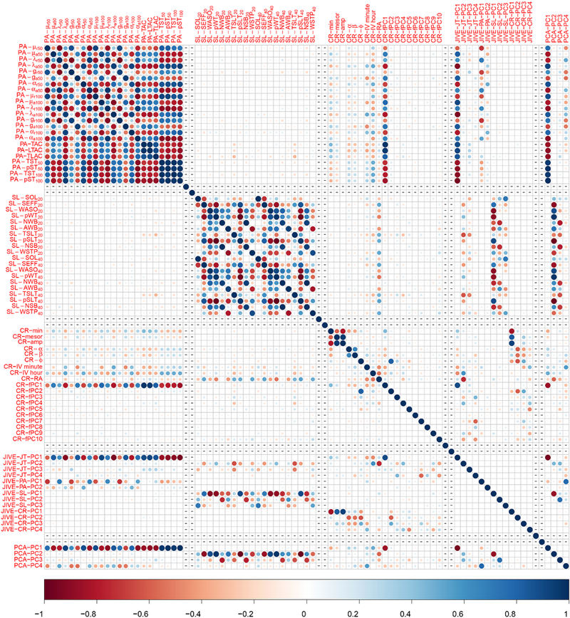
Both PCA and JIVE provide principal component scores, projections of the original data onto the corresponding principal components. Below, we denote a joint JIVE score by “JT-PC” and an individual score corresponding to one of the domains by “PA/SL/CR-PC”. Figure 8 shows the cross-correlation between all features, the 13 joint and individual JIVE scores and top 4 PC scores from PCA. It is obvious that there is extremely high correlation between features within both the PA and the SL domains. However, the level of correlation in the CR domain is not as high. This is expected because the first 10 functional PC scores have been included to represent this domain. Surprisingly, there is a very low cross-correlation between features of PA and SL domains. Moreover, all features in the PA domains display relatively high correlation with majority of features in CR. This correlation is particularly strong between PA and the first functional PC scores (fPCl), which typically shows the average diurnal profile. As shown in A.1 in Appendix A, fPCl corresponds to overall activity level during waking hours (approximately 6AM to 12AM), the time period where the features of PA domain were derived for majority of participants. We observed that JT-PC1 is highly correlated with majority of features from PA, and some features from CR (especially fPCl), but hot correlated with SL features. This is consistent with our finding such that the first Joint PC primarily represents PA and CR, but not SL. On the other hand. JT-PC2 and JT-PC3 represent significant variation of SL domain. Figure 9 shows the age-related change of joint and individual JIVE scores. Clear age trends can be seen for most of the derived JIVE scores with specific landmarks, such as lows and highs and changes in the observed trends.

Fig. 8.

Cross-correlations between twenty three PA features, twenty SL features, nineteen CR features, four JIVE-joint scores, two JIVE-PA scores, three JIVE-SL scores, four JIVE-CR scores, and four PC scores.

Fig. 9.

Relationship between age and joint/individual scores. Black solid lines are smoothing curve fitted using loess.

Unlike the original features that demonstrate significant correlation, the derived JIVE scores are orthogonal by construction. Similar to how PCA scores are used in the principal component regression to substitute original covariates with PC scores. JIVE scores can be used in the same way.

To illustrate this, we studied the association between usual gait speed (a commonly used indicator of physical function/performance) and scores from PCA (PCA-regression) and JIVE (JIVE-regression). Both PCA and JIVE scores are uncorrelated by construction, therefore, we can include all of them as covariates without worrying about collinearity. Baseline model (Model 0) contains age. gender, and body mass index (BMI) as covariates. Models 1 and 2 expand the baseline model with PCA and JIVE scores, respectively. The results for all three models are shown in Table 4. In general, the JIVE-regression resulted in a higher adjusted- R² of 0.33 compared to adjusted-R² of 0.29 for PCA-regression. However, this could be partially due to the smaller number of PCA components. In the model with PCA scores, PCA-PC1 and PCA-PC4 are negatively associated with gait speed. PCA-PC1 is highly loaded on all features in PA domain, while PCA-PC4 is slightly loaded on almost all features in all three domains. Thus, the interpretation of PCA-regression is quite complicated because it involves almost all features. JIVE-regression provides 0.09 increase in the adjusted-R² compared to the baseline model. Because all scores are uncorrelated and normalized, the magnitude of regression coefficients can be approximately interpreted as a contribution to the increase of the adjusted-R². First, JIVE-JT-1 is highly negatively correlated with PCA-PC1, thus, this finding is similar to PCA-regression. However, significant scores JIVE-PA-2 in PA domain and JIVE-SL-2 and JIVE-SL-3 in SL domain together contribute more than a half to the increase of the adjusted-R2. JIVE-PA-2 is highly loaded on all fragmentation metrics of physical activity and JIVE-SL-2 and JIVE-SL-3 are highly loaded on the fragmentation of sleep and do not include any metrics characterizing sleep efficiency. Thus, the results highlight the features quantifying patterns of fragmentation both during wake and during sleep as independently associated with gait speed. Interestingly, this is consistent with a recent finding of a negative association between the gait speed and the fragmentation of physical activity (measured by λ_a, i.e. activity to sedentary transition probability), such that increasing of λ_a is associated with a slower gait speed (Schrack et al, 2018a). To the best of our knowledge, the association between gait speed and the sleep characteristics have not been studied. Thus, JIVE-regression allows to separate domain-specific sources of variability and model their independent association with the outcome of interest while addressing possible multicollinearity.

Table 4.

Regression modelling of gait speed and PCA and JIVE Scores.

Model	Covariates	β	p-value	Adjusted R2
Model 0	BMI	−0.079	0.21	0.24
	Age	−0.50	<0.0001
	Female	−0.31	0.016
Model 1	PC1	−0.17	0.0069	0.29
	PC2	−0.031	0.61
	PC3	−0.11	0.075
	PC4	−0.14	0.022
Model 2	JIVE-JT-1	0.21	0.00096	0.33
	J1VE-JT-2	−0.061	0.33
	J1VE-JT3	0.036	0.56
	J1VE-JT4	−0.0055	0.93
	J1VE-PA-1	−0.016	0.79
	JIVE-PA-2	0.15	0.012
	JlVE-SL-1	−0.019	0.75
	JIVE-SL-2	−0.14	0.024
	JIVE-SL-3	0.13	0.033
	J1VE-CR-1	−0.016	0.79
	JIVE-CR-2	0.14	0.023
	J1VE-CR3	0.049	0.34
	J1VE-CR4	−0.094	0.11

^*Model 0 is the baseline model with age, gender, and BMI. Models 1 and 2 include PCA-PC and JIVE scores, respectively. All continuous variables (age, BMI, and all scores) have been centered and normalized.

We also explored a simple alternative to JIVE by using a two-step procedure: 1) performing PCA to each individual domain and 2) applying JIVE to the joint truncated data representing all three domains. To keep high enough percent of variation and to be able to potentially recover structures similar to original JIVE, we considered two scenarios for step one (PCA for individual domains): 1) keeping 5 PCs in each domain and 2) keeping 8 PCs in each domain. The full results are provided in Section B of the Appendix.

We believe this approach may have two limitations. First, it requires rank selection both at step 1 (PCA for individual domains) and step 2 (JIVE to truncated data). This seems to introduce extra uncertainty. Second, if we do not keep a sufficiently large number of PCs for each domain, this can result in not capturing some parts of joint variation. One intuitive analogy is Principal Component Regression (PCR) that does PCA on covariates at step 1 and regress PC scores on an outcome at step 2. PCR has no guarantee that variation kept at Step 1 is relevant to variation of the outcome. In our settings. PCA done in each individual domain are not informed by variation from other domains and. thus, in the same way as PCR, may discard a part of joint variation.

4.4. Sensitivity Analyses to Missing Data

In the main analysis, we follow the convention for BLSA actigraphy data processing pipeline to handle missingness in raw minute-level AC data. Specifically, days with more than 5% of missingness (more than 72 minutes per day) were treated as invalid and excluded from the analysis. For the days with less than 5% of missing data, missing values were imputed as the average activity counts per minute over all valid days at the same period for each participant.

In this section, we conduct sensitivity analyses using alternative ways of handling missing data. In sensitivity analysis 1 (denoted by SI), missing data were imputed using median of the specific time for each participant. We still have 198 subjects with the total of 1134 valid days (the mean is 5.72 days and standard deviation is 0.62). In sensitivity analysis 2 (denoted by S2), instead of using 5% of the threshold, we excluded days with more than 7% of missing data (101 minutes per day). We have 198 subjects with the total of 1163 days (the mean is 5.76 days and standard deviation is 0.59). In sensitivity analysis 3 (denoted by S3), we considered the most aggressive approach that removed all days with any missing data. This approach resulted in 189 subjects with the total 986 days (the mean is 5.22 days and standard deviation is 0.98).

All three approaches provided the results very similar to the results in the main analysis. In all three sensitivity analyses, JIVE chose joint rank to be 4, and individual ranks for PA/SL/CR domains to be 2, 3, and 4, respectively. Fig 10 displays bar-charts of the amount of variation explained by joint and individual components in each of the three domains. PA is dominated by the joint variation, SL is dominated by individual variations, and a significant amount of variation remained unexplained in CR domain.

Fig. 10.

Joint and individual variations explained by each domain from JIVE for S1 - S3. Results of all the three sensitivity analyses are similar to the variation pattern in the main analysis.

Figures C.1 – C.3 in the appendix display the cross-correlation plots between features and JIVE/PCA scores. The patterns are quite similar to what we observed from main analysis as well.

5. Discussion

We proposed to use JIVE to model individual and joint variation of domains of physical activity, sleep, and circadian rhythmicity represented by multiple domain-specific actigraphy-derived features. Using the BLSA study, we estimated and separated joint and individual components and scores and examined the correlation between those scores and the original features. We also explored age-specific changes of the scores and their association with usual gait speed. To the best of our knowledge, this is the first attempt to simultaneously model the domains of PA, SL, and CR using JIVE.

Our results demonstrate that the first JIVE Joint PC (JT-PC1) primarily represents shared PA and CR variation. Recent studies have shown that fPGl, which is also highly correlated with JIVE-JT-PC1, can be used as a biomarker for “biological age” (Pyrkov et, al, 2018). Even though JIVE is developed to identify joint variation across all three domains, this is an interesting finding. This can be further investigated by applying recently developed “structural learning and integrative decomposition’ (Gaynanova and Li, 2017) that estimates partially shared variation by assuming certain block-sparsity across domains.

Visual exploration of age-related changes in JIVE scores revealed interesting trends across joint and individual JIVE scores. These trends may provide additional insights in studies of PA/SL/GR that look at age effects, and try to understand joint and individual effects to each domain. This deserves further analyses and proper regression modeling in the future to identify a more rigorous relationship between age and the joint and individual scores.

From regression modeling perspective, JIVE provides joint and individual scores that can be included simultaneously in regression models as covariates, which can be seen as an extension of the standard principal component regression (Kaplan and Lock, 2017). A big advantage of JIVE is its ability to separate joint and individual variation and to explore associations between domain-specific variation and outcomes. As an example, we studied the association between usual gait speed with PCA and JIVE scores. The results showed that features quantifying patterns of fragmentation both during wake and sleep time were independently associated with gait speed, which supports results from a recent study (Schrack et al. 2018a). Thus, our results demonstrate the potential of JIVE to reveal important biological mechanisms in the joint context of PA. SL, and CR.

It is important to note that. JIVE, similar to PCA. is an unsupervised, data-driven approach for dimension reduction, which depends on pre-selected features and. potentially, the study sample (Ringnér. 2008). Therefore, when JIVE results are interpreted, it is crucial to understand that the inferences are based on pre-selected features. Even though we tried to incorporate a comprehensive list of commonly used features, the research fields of physical activity, sleep, and circadian rhythmicity are under a rapid development with a constant in-flow of novel summaries. Therefore, the number of features within each domain is expected to increase drastically. A big advantage of JIVE is that it efficiently handles redundancy of highly correlated features. Thus, for those features that require thresholding of AC or depend on a parameter which needs to be tuned or there is an interest in considering multiple time scale, it is possible to include several features corresponding to a wide grid of thresholds/parameters/time scales and eliminate created redundancy through JIVE. This is important because i) this eliminates the need for choosing thresholds/parameters and ii) different thresholds/parameters may correspond to different aspects of the phenomena of interest. It is also important to note that BLSA is a study of healthy aging and on average tend to focus on healthier sub-population, so the results in another cohort may be different.

Surprisingly, in our study the cross-correlation between domains of PA and SL was small. There are a few possible explanations of this. First, it may be due to nonlinear relationships between features of PA and SL. For example, it has been shown that the total sleep time usually exhibits a U-shaped association with various health outcomes such as obesity, diabetes, heart disease, and mortality (Taheri et al. 2004: Kripke et al. 2002: Patel et al. 2012: Ayas et al. 2003a.b). Second, domain-specific features were generated by averaging across valid days, which likely resulted in damping dynamic associations between adjacent sleep-wake periods. Thus, potentially strong within-week temporal patterns clustered within subjects were averaged out. Estimating those weekly temporal patterns and incorporating them into JIVE will need to be done as a next step.

JIVE can be readily extended to include an arbitrary number of domains. This is especially important considering the active embedding of multiple sensors in wearables for multi-domain tracking of physical activity, ambient light, skin temperature, sweat, blood pressure, glucose, heart rate, and many others.

There are a few limitations. First. JIVE only accounts for second-order correlation structure and ignores higher order mutual dependencies that may be quite informative when dealing with continuous multivariate non-Gaussian data. Second. JIVE is not capable of working with features that follow discrete distributions such as binary. Poisson. ordinal or categorical distributions. Third. JIVE only models joint and individual patterns without accounting for partially-shared structure, when, for example, two domains can share a joint component that is not present in the third domain. Thus, future work will need to focus on developing and applying methods that decompose joint dependence structure using measures of higher-order dependency such as multivariate skewness and kurtosis (Morton and Lirn. 2009: Jondeau et al. 2010: Miettinen et al. 2015) and capable of handing mixed data-types (Tran et al. 2011: Udell et al. 2016: Li and Gaynanova. 2017) and accounting for partially shared structure (Gaynanova and Li. 2017).

In summary, our proposal of using JIVE to model the domains of PA, SL, and CR is an important step forward to provide analytical methods for multi-feature multi-domain wearable data that will facilitate our understanding of complex interactions of multiple physiological systems.

A. Functional PCA

Functional PCs for circadian rhythmicity domain, for each subject, 1440-minute activity profile were averaged across valid days which resulted in an average daily profile that is representative. Then functional PC A using sandwich smoother for covariance matrix smoothing was applied (Xiao et al, 2016). The first 10 principal components explained more than 90% of total variation.Figure A.1 shows the first 10 functional PCs.

Fig. A.1.

First 10 functional principal components reported with cumulative variance explained.

B. Results from the Two-Step Alternative Approach

We considered an alternative two-step approach by first performing PC A to each domain individually, and then applying JIVE to the joint truncated data from all three domains.

In order to keep as much joint variation as possible, we considered in the first step (i.e. individual PCA) to keep 5 and 8 PCs from each domain. When 5 PCs were kept in each domain, JIVE selected joint rank to be 4,

Fig. B.1.

Joint and individual variations explained by each domain from the alternative approach to conduct JIVE, a): 5 PCs were kept from the first step. Joint structure explains 87.3%. 49.8%, and 19.6% of total variation in PA, SL, and CR domains respectively. Individual structures explain 9.6%, 48.2%, and 79.8% of total variation in PA, SL, and CR domains, respectively. And there are only 3.2%, 2.0%, and 0.5% of variation that cannot be explained in PA, SL, and CR respectively, b): 8 PCs were kept from the first step. Joint structure explains 64.4%, 58.6%, and ‘21.6% of total variation in PA, SL, and CR domains respectively. Individual structures explain 31.4%, 37.3%, and 76.4% of total variation in PA, SL, and CR domains, respectively. And there are only 4.2%, 4.1%, and 2.0% of variation that cannot be explained in PA, SL, and CR respectively.

and 1, 2, and 5 as the individual ranks for PA, SL, and CR respectively. Meanwhile, when 8 PCs were kept in each domain, JIVE selected joint rank to be 4 as well, but individual ranks to be 2, 2, and 7 for domains for PA, SL, and CR respectively. Figure B.1 shows the proportion of variation explained. Even though it seems like there are more joint variation recovered, but we have to keep in mind that, potentially useful information may have been removed, and the proportion here is with respect to the remained variation in the truncated data.

Figures B.2 and B.3 show the relationships between JIVE results from the main analysis (denoted by (A)) and the alternative analysis with 5 PCs selected (denoted by (B1)), and with 8 PCs selected (denoted by (B2)). The first joint PCs between (A) and (B1)/(B2) are highly correlated, which shows high consistency between the two approaches. There is also certain level correlation between JT-PC2 from the two approaches. The individual PCs from the two approaches are highly correlated.

C. Results for the Sensitivity Analyses

This section contains the results from the sensitivity analyses described in Section 4.4 where we considered 3 other ways to handle missing data in activity profiles. In sensitivity analysis 1 (SI), missing data were imputed using median of the specific time within each subject instead of mean. We still have 198 subjects contributed by 1134 days (with mean 5.72 days and standard deviation of 0.62). In sensitivity analysis 2 (S2), instead of using 5% of the threshold, we consider removing days with more than 7% of missing data (101 minutes per day). We have 198 subjects contributed by 1163 days (with mean 5.76 days and standard deviation of 0.59).In sensitivity analysis 3 (S3), we considered the most aggressive approach which is to remove all subject-days with missing values. This approach left us 189 subjects contributed by 986 days (with mean 5.22 days and standard deviation of 0.98).

The patterns are quite similar to what we observed from the main analysis. In SI, joint structure explains 68.1%, 20.1%, and 25.8% of total variation in PA, SL, and CR domains respectively. Individual structures explain 26.1%, 74.5%, and 38.5% of total variation in PA, SL, and CR domains, respectively. And there are only 5.8%, 5.3%, and 35.7% of variation that cannot be explained in PA, SL, and CR respectively. In S2, joint structure explains 69.0%, 18.7%, and 25.9% of total variation in PA, SL, and CR domains respectively. Individual structures explain 25.2%, 76.2%, and 38.6% of total variation in PA, SL, and CR domains, respectively. And there are only 5.7%, 5.2%, and 35.5% of variation that cannot be explained in PA, SL, and CR respectively. Finally, in S3, joint structure explains 63.6%, 20.7%, and 27.2% of total variation in PA, SL, and CR domains respectively. Individual structures explain 30.5%, 73.0%, and 35.3% of total variation in PA, SL, and CR domains, respectively. And there are only 6.0%, 6.3%, and 37.5% of variation that cannot be explained in PA, SL, and CR respectively. The cross-correlation plots between features and JIVE/PC scores are shown in Figures C.1 -C.3.

Fig. B.2.

Cross-correlations between (A) original JIVE and (B1) two-step JIVE with 5 PCs selected in the first step

Fig. B.3.

Cross-correlations between (A) original jive and (B2) two-step jive with 8 PCs selected in the first step

Fig. C.1.

Cross-correlations between features and JIVE/PC scores, for S1, where median is used to impute missing data

Fig. C.2.

Cross-correlations between features and JIVE/PC scores, for S2, where days with more than 7% were removed

Fig. C.3.

Cross-correlations between features and JIVE/PC scores, for S3, wher all subject days with missing values were removed

References

- Actigraph (2018a) What are counts URL https://actigraph.desk.com/customer/en/portal/articles/2515580-what-are-counts-
- Actigraph (2018b) What does the “detect sleep periods” button do and how does it work? URL https://actigraph.desk.com/customer/en/portal/articles/2515836-what-does-the-%22detect-sleep-periods%22-button-do-and-how-does-it-work-
- Ancoli-Israel S Martin JL, Blackwell T, Buenaver L, Lin L, Meitzer LJ Sadeh A Spira AP, Taylor DJ (2015) The sbsrn guide to actigraphy monitoring: clinical and research applications. Behavioral sleep medicine 13(supl):S4–S38 [DOI] [PubMed] [Google Scholar]
- Argiropoulou EC. Michalopoulou M, Aggeloussis N, Avgerinos A (2004) Validity and reliability of physical activity measures in greek high school age children. Journal of sports science & medicine 3(3): 147. [PMC free article] [PubMed] [Google Scholar]
- Ayas NT, White DP, Al-Delainiy WK, Manson JE, Stampfer MJ, Speizer FE, Patel S, Hu FB (2003a) A Prospective Study of Self-Reported Sleep Duration and Incident Diabetes in Women. Diabetes Care 26(2):380–384, DOI 10.2337/diacare.26.2.380, URL http://care,diabetesjournals.org/cgi/doi/10.2337/diacare.26.2.380 [DOI] [PubMed] [Google Scholar]
- Ayas NT, White DP, Manson JE, Stampfer MJ, Speizer FE, Malhotra A, Hu FB (2003b) A Prospective Study of Sleep Duration and Coronary Heart Disease in Women. Archives of Internal Medicine 163(2):205, DOI 10.1001/archinte.l63.2.205, URL http://archinte.jamanetwork.com/article.aspx?doi=10.1001/archinte.163.2.205 [DOI] [PubMed] [Google Scholar]
- Bai J, Di C, Xiao L, Evenson KR, LaCroix AZ, Crainiceanu CM, Buchner DM (2016) An Activity Index for Raw Accelerometry Data and Its Comparison with Other Activity Metrics. PLOS ONE 11(8):e0160,644, DOI 10.1371journal.pone.0160644,11 URL http://dx.plos.org/10.1371/journal.pone.0160644 [DOI] [PMC free article] [PubMed] [Google Scholar]
- Bassett DR (2012) Device-based monitoring in physical activity and public health research. Physiological Measurement 33(11 ):1769–1783, DOI 10.1088/0967-3334/33/11/1769, URL http://stacks.iop.org/0967-3334/33/i=ll/a=1769?key=crossref.b7c0c2fa4d411e3007196cfla2351fa2 [DOI] [PubMed] [Google Scholar]
- Bassett DR, Troiano RP, McClain JJ, Wolff DL (2015) Accelerometer-based physical activity: total volume per day and standardized measures. Med Sei Sports Exerc 47(4):833–8 [DOI] [PubMed] [Google Scholar]
- Bellettiere J, Winkler EA, Chastin SF, Kerr J, Owen N, Dunstan DW, Healy GN (2017) Associations of sitting accumulation patterns with cardio-metabolic risk biomarkers in australian adults. PloS one 12(6):e0180,119 [DOI] [PMC free article] [PubMed] [Google Scholar]
- Buman MP, Winkler EAH, kurka JM, Hekler EB, Baldwin CM, Owen N, Ainsworth BE, Healy GN, Gardiner PA (2014) Reallocating Time to Sleep, Sedentary Behaviors, or Active Behaviors: Associations With Cardiovascular Disease Risk Biomarkers, NHANES 2005–2006. American Journal of Epidemiology 179(3):323–334, DOI 10.1093/ajc/kwt292, URL https://academic.oup.com/aje/article-lookup/doi/10.1093/aje/kwt292 [DOI] [PubMed] [Google Scholar]
- Chau JY, Grunseit AC, Chey T, Stamatakis E, Brown WJ, Matthews CE, Bauman AE, van der Ploeg HP (2013) Daily Sitting Time and All-Cause Mortality: A Meta-Analysis. PLoS ONE 8(ll):e80,000, DOI 10.1371/journal.pone.0080000, URL http://dx.plos.org/10.1371/journal.pone.0080000 [DOI] [PMC free article] [PubMed] [Google Scholar]
- Cornelissen G (2014) Cosinor-based rhythmomctry. Theoretical Biology and Medical Modelling 11 (1): 16. [DOI] [PMC free article] [PubMed] [Google Scholar]
- Di J, Leroux A, Urbanek J, Varadhan R, Spira A, Schrack J, Zipunnikov V (2017) Patterns of sedentary and active time accumulation are associated with mortality in US adults: The NHANES study. bioRxiv URL http://biorxiv.org/content/early/2017/08/31/182337. [Google Scholar]
- Diaz KM, Howard VJ, Hutto B, Colabianchi N, Vena JE, Safford MM, Blair SN, Hooker SP (2017) Patterns of Sedentary Behavior and Mortality in U.S. Middle-Aged and Older Adults. Annals of Internal Medicine DOI 10.7326/M17-0212, URL http://annals.org/article.aspx?doi=10.7326/M17-0212 [DOI] [PMC free article] [PubMed] [Google Scholar]
- Dunlap JC, Loros JJ, DeCoursey PJ (2004) Chronobiology: biological timekeeping. Sinauer Associates [Google Scholar]
- Dunstan DW, Kingwell BA, Larsen R, Healy GN, Cerin E, Hamilton MT, Shaw JE, Bertovic DA, Zinimet PZ, Salmon J, Owen N (2012) Breaking Up Prolonged Sitting Reduces Postprandial Glucose and Insulin Responses. Diabetes Care 35(5):976–983, DOI 10.2337/dcll-1931, URL http://care.diabetesjournals.org/cgi/doi/10.2337/dcll-1931 [DOI] [PMC free article] [PubMed] [Google Scholar]
- Edgar RS, Green EW, Zhao Y, van Ooijen G, Olmedo M, Qin X, Xu Y, Pan M, Valekunja UK, Feeney KA, Maywood ES, Hastings MH, Baliga NS, Merrow M, Millar AJ, Johnson CH, Ivyriacou CP, O’Neill JS, Reddy AB (2012) Peroxiredoxins are conserved markers of circadian rhythms. Nature DOI 10.1038/naturell088, URL http://www.nature.com/doifinder/10.1038/naturell088 [DOI] [PMC free article] [PubMed] [Google Scholar]
- Feng Q, Hannig J, Marron J (2015) Non-iterative joint and individual variation explained. arXiv preprint arXiv:151204060 [Google Scholar]
- Ferrucci L (2008) The Baltimore Longitudinal Study of Aging (BLSA): A 50-Year-Long Journey and Plans for the Future. The Journals of Gerontology Series A: Biological Sciences and Medical Sciences 63(12):1416–1419, DOI 10.1093/gcrona/63.12.1416, URL https://academic.oup.com/biomedgerontology/article-lookup/doi/10.1093/gerona/63.12.1416 [DOI] [PMC free article] [PubMed] [Google Scholar]
- Ferrucci L, Alley D (2007) Obesity, disability, and mortality: a puzzling link. Archives of internal medicine 167(8):750–751 [DOI] [PMC free article] [PubMed] [Google Scholar]
- Gaynanova I, Li G (2017) Structural learning and integrative decomposition of multi-view data. arXiv preprint arXiv: 170706573 [DOI] [PubMed] [Google Scholar]
- Goldsmith J, Zipunnikov V, Schrack J (2015) Generalized multilevel function-on-scalar regression and principal component analysis. Biometrics 71(2):344–353 [DOI] [PMC free article] [PubMed] [Google Scholar]
- Gonçalves BS, Cavalcanti PR, Tavares GR, Campos TF, Araujo JF (2014) Nonparametric methods in actigraphy: An update. Sleep Science 7(3): 158–164 [DOI] [PMC free article] [PubMed] [Google Scholar]
- Hamilton MT, Healy GN, Dunstan DW, Zderic TW, Owen N (2008) Too little exercise and too much sitting: Inactivity physiology and the need for new recommendations on sedentary behavior. Current Cardiovascular Risk Reports 2(4):292–298, DOI 10.1007/sl2170-008-0054-8, URL http://link.springer.com/10.1007/s12170-008-0054-8 [DOI] [PMC free article] [PubMed] [Google Scholar]
- Hauri PJ, Wisbey J (1992) Wrist Actigraphy in Insomnia. Sleep 15(4):293–301, DOI 10.1093/sleep/15.4.293, URL https://academic.oup.com/sleep/article-lookup/doi/10.1093/sleep/15.4.293 [DOI] [PubMed] [Google Scholar]
- Healy GN, Clark BK, Winkler EA, Gardiner PA, Brown WJ, Matthews GE (2011) Measurement of Adults’ Sedentary Time in Population-Based Studies. American Journal of Preventive Medicine 41 (2):216–227, DOI 10.1016/j.amepre.2011.05.005, URL http://linkinghub.elsevier.com/retrieve/pii/S0749379711003138 [DOI] [PMC free article] [PubMed] [Google Scholar]
- van Hees VT, Sabia S, Jones SE, Wood AR, Anderson KN, Kivimäki M, Frayling TM, Pack AI, Bucan M, Trenell M, et al. (2018) Estimating sleep parameters using an accelerometer without sleep diary. Scientific reports 8(1 ):12,975 [DOI] [PMC free article] [PubMed] [Google Scholar]
- Hofstra WA, de Weerd AW (2008) How to assess circadian rhythm in humans: A review of literature. Epilepsy & Behavior 13(3):438–444, DOI 10.1016/j.yebeh.2008.06.002, URL http://linkinghub.elsevier.com/retrieve/pii/S1525505008001625 [DOI] [PubMed] [Google Scholar]
- Hotelling H (1936) Relations Between Two Sets of Variates. Biometrika 28(¾):321, DOI 10.2307/233395S, URL http://www.jstor.org/stable/2333955?origin=crossref [DOI] [Google Scholar]
- Joan-Louis G, von Gizycki H, Zizi F, Fookson J, Spielman A. Nunes J, Fullilove R, Taub H (1996) Determination of sloop and wakofnlnoss with tho actigraph data analysis softwaro (ADAS). Sloop 19(9):739–43. URL http://www.ncbi.nlm.nih.gov/pubmed/9122562 [PubMed] [Google Scholar]
- Joan-Louis G, Kripke DF, Cole RJ, Assmus JD, Langor RD (2001) Sleep detection with an acceleronieter actigraph: comparisons with polysomnography. Physiology & Behavior 72(1– 2):21–28. DOI 10.1016/S0031-9384(00)00355-3, URL http://linkinghub.elsevier.com/retrieve/pii/S0031938400003553 [DOI] [PubMed] [Google Scholar]
- John D, Froodson P (2012) ActiGraph and Actical physical activity monitors: a peek under the hood. Medicine and science in sports and exercise 44(1 Suppl 1):S86–9. DOI 10.1249/MSS.0b013e3182399f5e, URL http://www.ncbi.nlm.nih.gov/pubmed/22157779http://www.pubmedcentral.nih.gov/articlerender.fcgi?artid=PMC3248573 [DOI] [PMC free article] [PubMed] [Google Scholar]
- Jondeau E, Jurczenko E, Rockinger M (2010) Moment Component Analysis: An Illustration with International Stock Markets. SSRN Electronic Journal DOI 10.2139/ssrn.1694643 URL http://www.ssrn.com/abstract=1694643 [DOI] [Google Scholar]
- Kaplan A Lock EF (2017) Prediction with dimension reduction of multiple molecular data sources for patient survival. arXiv preprint arXiv: 170402069 [DOI] [PMC free article] [PubMed] [Google Scholar]
- Koster A Caserotti P Patel KV, Matthews CE, Berrigan D, Van Domelen DR Brychta RJ Chen KY, Harris TB (2012) Association of Sedentary Time with Mortality Independent of Moderate to Vigorous Physical Activity. PLoS ONE 7(6):e37,696, DOI 10.1371/journal.pone.0037696 URL http://dx.plos.org/10.1371/journal.pone.0037696 [DOI] [PMC free article] [PubMed] [Google Scholar]
- Kripke DF. Garfinkel L, Wingard DL, Klauber MR, Marler MR (2002) Mortality Associated With Sleep Duration and Insomnia. Archives of General Psychiatry 59(2):131, DOI 10.1001/archpsyc.59.2.131, URL http://archpsyc.jamanetwork.com/article.aspx?doi=10.1001/archpsyc.59.2.131 [DOI] [PubMed] [Google Scholar]
- Kushida CA, Chang A, Gadkary C, Guilleminault C, Carrillo O, Dement WC (2001) Comparison of actigraphic, polysomnographic, and subjective assessment of sleep parameters in sleep-disordered patients. Sleep Medicine 2(5):389–396, DOI 10.1016/S1389-9457(00)00098-8, URL http://linkinghub.elsevier.com/retrieve/pii/S1389945700000988 [DOI] [PubMed] [Google Scholar]
- Loroux A, Di J, Smirnova E, Mcguffey EJ, Cao Q, Bayatmokhtari E, Tabacu L, Zipunnikov V, Urbanek JK, Crainiceanu C (2019) Organizing and Analyzing the Activity Data in NHANES. Statistics in Biosciences DOI , URL http://link,springer.com/10.1007/s12561-018-09229-9 [DOI] [PMC free article] [PubMed] [Google Scholar]
- Li G, Gaynanova I (2017) A general framework for association analysis of heterogeneous data. arXiv preprint arXiv: 170706485 [Google Scholar]
- Lock EF, Hoadley KA, Marron JS, Nobel AB (2013) Joint and individual variation explained (JIVE) for integrated analysis of multiple data types. The Annals of Applied Statistics 7(1):523–542, DOI 10.1214/12-AOAS597, URL http://projecteuclid.org/euclid.aoas/1365527209 [DOI] [PMC free article] [PubMed] [Google Scholar]
- Marler MR, Gohrman P, Martin JL, Ancoli-Israel S (2006) The sigmoidally transformed cosine curve: a mathematical model for circadian rhythms with symmetric non-sinusoidal shapes. Statistics in Medicine 25(22):3893–3904, DOI 10.1002/sim.2466, URL http://doi.wiley.com/10.1002/sim.2466 [DOI] [PubMed] [Google Scholar]
- Matthews CE, George SM, Moore SC, Bowles HR, Blair A, Park Y, Troiano RP, Hollenbeck A, Schatzkin A (2012) Amount of time spent in sedentary behaviors and cause-specific mortality in US adults. American Journal of Clinical Nutrition 95(2):437–445, DOI 10.3945/ajcn.lll.019620, URL http://www.ajcn.org/cgi/doi/10.3945/ajcn.Ill.019620 [DOI] [PMC free article] [PubMed] [Google Scholar]
- Miettinen J, Taskinen S, Nordhausen K, Oja H (2015) Fourth Moments and Independent Component Analysis. Statistical Science 30(3):372–390, DOI 10.1214/15-STS520, URL http://projecteuclid.org/euclid.ss/1439220718 [DOI] [Google Scholar]
- Mills JN (1966) Human circadian rhythms. Physiological reviews 46( 1): 128–171 [DOI] [PubMed] [Google Scholar]
- Morton J, Lini LH (2009) Principal cunmlant component analysis, preprint [Google Scholar]
- Nakazaki K, Kitamura S. Motomura Y, Hida A Kamei Y, Miura N, Mishima K (2014) Validity of an algorithm for determining sleep/wake states using a new actigraph. Journal of Physiological Anthropology 33(1):31, DOI 10.1186/1880-6805-33-31, URL http://jphysiolanthropol.biomedcentral.com/articles/10.1186/1880-6805-33-31 [DOI] [PMC free article] [PubMed] [Google Scholar]
- Nastasi AJ, Ahuja A, Zipunnikov V, Simonsick EM, Ferrucci L, Schrack JA (2018) Objectively Measured Physical Activity and Falls in Well-Functioning Older Adults. American Journal of Physical Medicine & Rehabilitation 97(4):255–260, DOI 10.1097/PHM.0000000000000830, URL http://insights.ovid.com/crossref?an=00002060-201804000-00005 [DOI] [PMC free article] [PubMed] [Google Scholar]
- Owen N, Healy GN, Matthews CE, Dunstan DW (2010) Too much sitting: the population- health science of sedentary behavior. Exercise and Sport Sciences Reviews 38(3):105–113, DOI 10.1097/JES.0b013e3181e373a2, URL http://content.wkhealth.com/linkback/openurl?sid=WKPTLP:landingpage{&}an=00003677-201007000-00003 [DOI] [PMC free article] [PubMed] [Google Scholar]
- Patel SR, Malhotra A, Gao X, Hu FB, Neuman MI, Fawzi WW (2012) A Prospective Study of Sleep Duration and Pneumonia Risk in Women. Sleep 35(1):97–101, DOI 10.5665/sleep.1594, URL https://academic.oup.com/sleep/article-lookup/doi/10.5665/sleep.1594 [DOI] [PMC free article] [PubMed] [Google Scholar]
- Pyrkov TV, Slipensky K, Barg M, Kondrashin A, Zhurov B, Zenin A, Pyatnitskiy M, Menshikov L, Markov S, Fedichev PO (2018) Extracting biological age from biomedical data via deep learning: too much of a good thing? Scientific reports 8(1 ):5210. [DOI] [PMC free article] [PubMed] [Google Scholar]
- Ramsay JO (2006) Functional data analysis. Wiley Online Library [Google Scholar]
- Ringnér M (2008) What is principal component analysis? Nature Biotechnology 26(3):303–304, DOI 10.1038/nbt0308-303, URL http://www.nature.com/articles/nbt0308-303 [DOI] [PubMed] [Google Scholar]
- Schrack JA, Zipunnikov V, Goldsmith J, Bai J, Simonsick EM, Crainiceanu C, Ferrucci L (2014) Assessing the “Physical Cliff”: Detailed Quantification of Age-Related Differences in Daily Patterns of Physical Activity. The Journals of Gerontology Series A: Biological Sciences and Medical Sciences 69(8):973–979, DOI 10.1093/gcrona/gltl99, URL https://academic.oup.com/biomedgerontology/article-lookup/doi/10.1093/gerona/gltl99 [DOI] [PMC free article] [PubMed] [Google Scholar]
- Schrack JA, Kuo PL, Wanigatunga AA, Di J, Simonsick EM, Spira AP, Ferrucci L, Zipunnikov V (2018a) Active-to-sedentary behavior transitions, fatigability, and physical functioning in older adults. The Journals of Gerontology: Series A [DOI] [PMC free article] [PubMed] [Google Scholar]
- Schrack JA, Leroux A, Fleg JL, Zipunnikov V, Simonsick EM, Studenski SA, Crainiceanu C, Ferrucci L (2018b) Using Heart Rate and Accelerometry to Define Quantity and Intensity of Physical Activity in Older Adults. The Journals of Gerontology: Series A 73(5):668–675, DOI 10.1093/gcrona/gly029, URL https://academic.oup.com/biomedgerontology/article/73/5/668/4917366 [DOI] [PMC free article] [PubMed] [Google Scholar]
- Shephard RJ (2003) Limits to the measurement of habitual physical activity by questionnaires * Commentary. British Journal of Sports Medicine 37( >3): 197–206, DOI 10.1136/bjsm.37.3.197, URL http://bjsm.bmj.com/cgi/doi/10.1136/bjsm.37.3.197 [DOI] [PMC free article] [PubMed] [Google Scholar]
- Shou H, Zipunnikov V, Crainiceanu CM, Greven S (2015) Structured functional principal component analysis. Biometrics 71 (1):247–257 [DOI] [PMC free article] [PubMed] [Google Scholar]
- van Someren EJ, Hagebeuk EE, Lijzenga C, Scheltens P, de Rooij SE, Jonker C, Pot AM, Mirmiran M, Swaab DF (1996) Circadian rest—activity rhythm disturbances in alzheimer’s disease. Biological Psychiatry 40(4):259–270, DOI 10.1016/0006-3223(95)00370-3, URL http://linkinghub.elsevier.com/retrieve/pii/0006322395003703 [DOI] [PubMed] [Google Scholar]
- Spira AP, An Y, Peng Y, Wu MN, Simonsick EM, Ferrucci L, Resnick SM (2017) Apoe genotype and nonrespiratory sleep parameters in cognitively intact older adults. Sleep 40(8) [DOI] [PMC free article] [PubMed] [Google Scholar]
- Stone JL, Norris AH (1966) Activities and Attitudes of Participants in the Baltimore Longitudinal Study. Journal of Gerontology 21 (4):575–580, DOI 10.1093/gcronj/21.4.575, URL https://academic.oup.com/geronj/article-lookup/doi/10.1093/geronj/21.4.575 [DOI] [PubMed] [Google Scholar]
- Taheri S Lin L, Austin D, Young T, Mignot E (2004) Short Sloop Duration Is Associatoci with Roducod Leptin, Elevated Ghrelin, and Increased Body Mass Index. PLoS Medicine 1(3):e62, DOI 10.1371/journal.pmod.0010062 URL http://dx.plos.org/10.1371/journal.pmed.0010062 [DOI] [PMC free article] [PubMed] [Google Scholar]
- Tilrnanno J, Urbain J, Kotharo MV, Wouwor AV, Kotharo SV (2009) Algorithms for sloop-wako identification using actigraphy: a comparativo study and now results. Journal of Sloop Research 18(1 ):85–98. DOI 10.llll/j.1365-2869.2008.00706.x URL http://doi.wiley.com/10.llll/j.1365-2869.2008.00706.x [DOI] [PubMed] [Google Scholar]
- Tran T, Phung D, Vonkatesh S (2011) Mixed-variate restricted boltzmann machines. In: Asian Conference on Machine Learning, pp 213–229 [Google Scholar]
- Tremblay MS, Aubort S, Barnes JD, Saunders TJ, Carson V, Latimor-Cheung AE, Chastin SF, Altenburg TM, Chinapaw MJ (2017) Sedentary Behavior Research Network (SBRN)–Terminology Consensus Project process and outcome. International Journal of Behavioral Nutrition and Physical Activity 14(1 ):75, DOI , URL http://ijbnpa.biomedcentral.com/articles/10.1186/sl2966-017-0525-8 [DOI] [PMC free article] [PubMed] [Google Scholar]
- Troiano R, Berrigan D, Dodd K, Masse L, Tilert T, McDowell M (2008) Physical activity in the united states measured by accelerometer. Med Sci Sports Exerc 40 ( 1 ) : 181. [DOI] [PubMed] [Google Scholar]
- Troiano RP, Macera CA, Ballard-Barbash R (2001) Be physically active each day. How can we know? The Journal of nutrition 131 (2S-1 ):451S–460S, URL http://www.ncbi.nlm.nih.gov/pubmed/11160577 [DOI] [PubMed] [Google Scholar]
- Udell M, Horn C, Zadeh R, Boyd S, et al. (2016) Generalized low rank models. Foundations and Trends® in Machine Learning 9(1):1–118 [Google Scholar]
- Urbanek JK, Spira AP, Di J, Leroux A, Crainiceanu C, Zipunnikov V (2018) Epidemiology of objectively measured bedtime and chronotype in us adolescents and adults: Nhanes 2003–2006. Chronobiology international 35(3):416–434 [DOI] [PMC free article] [PubMed] [Google Scholar]
- Van Somoren EJW, Swaab DF, Colenda CC, Cohen W, McCall WV, Rosenquist PB (1999) Bright Light Therapy: Improved Sensitivity to Its Effects on Rest-Activity Rhythms in Alzheimer Patients by Application of Nonparametric Methods. Chronobiology International 16(4):505–518, DOI 10.3109/07420529908998724, URL http://www.tandfonline.com/doi/full/10.3109/07420529908998724 [DOI] [PubMed] [Google Scholar]
- Varma VR, Dey D, Loroux A, Di J, Urbanek J, Xiao L, Zipunnikov V (2017a) Re-evaluating the effect of age on physical activity over the lifespan. Preventive Medicine [DOI] [PMC free article] [PubMed] [Google Scholar]
- Varma VR, Dey D, Loroux A, Di J, Urbanek J, Xiao L, Zipunnikov V (2017b) Total volume of physical activity: TAC, TLAC or TAC(A). Preventive medicine DOI 10.1016/j.ypmed.2017.10.028, URL http://www.ncbi.nlm.nih.gov/pubmed/29080825 [DOI] [PMC free article] [PubMed] [Google Scholar]
- Varo JJ, Martinez-Gonzáloz MA, de Irala-Estévez J, Kearney J, Gibney M, Martínez JA (2003) Distribution and determinants of sedentary lifestyles in the European Union. International Journal of Epidemiology 32( 1 ): 138–146, DOI 10.1093/ije/dygll6, URL https://academic.oup.com/ije/article-lookup/doi/10.1093/ije/dygll6 [DOI] [PubMed] [Google Scholar]
- Wanigatunga AA, Simonsick EM, Zipunnikov V, Spira AP, Studenski S, Ferrucci L, Schrack JA (2018) Perceived Fatigability and Objective Physical Activity in Mid- to Late-Life. The Journals of Gerontology: Series A 73(5):630–635, DOI 10.1093/gerona/glxl81, URL https://academic.oup.com/biomedgerontology/article/73/5/630/4168567 [DOI] [PMC free article] [PubMed] [Google Scholar]
- Witting W, Kwa I, Eikelenboom P, Mirmiran M, Swaab D (1990) Alterations in the circadian rest-activity rhythm in aging and alzhoimer’s disease. Biological psychiatry 27(6):563–572 [DOI] [PubMed] [Google Scholar]
- Wold H (2004) Partial Least Squares In: Encyclopedia of Statistical Sciences, John Wiley & Sons, Inc., Hoboken, NJ, USA, DOI 10.1002/0471667196.essl914, URL http://doi.wiley.com/10.1002/0471667196.essl914 [DOI] [Google Scholar]
- Wolff-Hughes DL. Fitzhugh EC. Bassett DR. Churilla JR (2015) Waist-worn actigraphy: population-referenced percentiles for total activity counts in us adults. Journal of Physical Activity and Health 12(4):447–453 [DOI] [PubMed] [Google Scholar]
- Xiao L Zipunnikov V. Ruppert D. Crainiceanu C (2016) Fast covariance estimation for high-dimensional functional data. Statistics and computing 26(l-2):409–421 [DOI] [PMC free article] [PubMed] [Google Scholar]