Rapidly Forming Early Intermediate Structures Dictate the Pathway of Capsid Assembly

Abstract

There are ∼10³⁰ possible intermediates on the assembly path from hepatitis B capsid protein dimers to the 120-dimer capsid. If every intermediate was tested, assembly would often get stuck in an entropic trap and essentially every capsid would follow a unique assembly path. Yet, capsids assemble rapidly with minimal trapped intermediates, a realization of the Levinthal paradox. To understand the fundamental mechanisms of capsid assembly, it is critical to resolve the early stages of the reaction. We have used time-resolved small angle X-ray scattering, which is sensitive to solute size and shape and has millisecond temporal resolution. Scattering curves were fit to a thermodynamically curated library of assembly intermediates, using the principle of maximum entropy. Maximum entropy also provides a physical rationale for the selection of species. We found that the capsid assembly pathway was exquisitely sensitive to initial assembly conditions. With the mildest conditions tested, the reaction appeared to be two-state from dimer to 120-dimer capsid with some dimers-of-dimers and trimers-of-dimers. In slightly more aggressive conditions, we observed transient accumulation of a decamer-of-dimers and the appearance of 90-dimer capsids. In conditions where there is measurable kinetic trapping, we found that highly diverse early intermediates accumulated within a fraction of a second and propagated into long-lived kinetically trapped states (≥90-mer). In all cases, intermediates between 35 and 90 subunits did not accumulate. These results are consistent with the presence of low barrier paths that connect early and late intermediates and direct the ultimate assembly path to late intermediates where assembly can be paused.

Introduction

A virus capsid is the protein shell that protects the genome of a virus. To minimize the amount of the viral genome devoted to structural proteins, capsids are composed of many copies of a small number of proteins, often only one.^1,2 Capsid assembly is a critical step in the life cycle of viruses. Despite years of research, the mechanism of icosahedral capsid assembly (about half of the known viruses) has remained poorly understood because it involves a large number of capsid protein subunits, a huge number of possible intermediates, and many more potential assembly pathways.³⁻⁵ The assembly process includes nucleation, elongation, and final closure, the time scale for which can cover many orders of magnitude: from milliseconds^6,7 to, in vitro, days.^8,9 The assembly pathways and their time scales are regulated by the interactions between the viral components, usually with no additional chaperone.¹⁰⁻¹³ The early reaction steps can be very fast, and hence, tracking them and resolving the involved structures can be challenging.^6,7,14,15 Experimental kinetic data at high temporal resolution, covering the early stages of assembly, are critical for resolving the underlying mechanism of virus assembly (and likewise disassembly).^{6,7,14,16−18}

For self-assembly of a hollow spherical polymer, capsid subunits must be able to form at least three intersubunit contacts.¹⁹ Subunits are often themselves small oligomers. Assembly theory and simulation^12,20−22 suggest that, for assembly to alleviate errors, follow the most efficient path, and avoid kinetic traps, association energy must be relatively weak, nucleation must be relatively slow, and association must be reversible. In practice, these regulatory features have an overlapping basis and can be controlled by solution conditions, adjusting association energy and/or protein concentration. By reference to classical polymerization theory,²³⁻²⁵ adjusting solution conditions modifies the initial subunit supersaturation of the system.

For this study, we examined the assembly of the hepatitis B virus (HBV) capsid because of the medical importance of the system, because its assembly in vitro is tractable, and because HBV capsid assembly has been identified as a promising target for direct-acting antiviral agents. HBV is an endemic pathogen that causes chronic infection in more than 250 million people and leads to about 880 000 deaths each year, by liver failure, cirrhosis, and liver cancer.²⁶ HBV is an enveloped dsDNA virus that has an icosahedral capsid composed of homodimeric core protein (Cp).²⁷In vivo, assembly can nucleate spontaneously to form empty particles, which comprise 90% of the particles present during infection.²⁸ The remaining population of infectious particles assembles around a complex of viral RNA and reverse transcriptase, which may itself play a role in catalyzing assembly nucleation.^29,30 Assembly directed antiviral agents, which include molecules now in clinical trials, act by accelerating assembly, strengthening association energy, and inducing aberrant geometry.³¹⁻³³

HBV assembly can be recapitulated with purified protein. Recombinant capsid protein assembly domain, Cp149, the first 149 residues of Cp, lacking the C-terminal nucleic acid binding domain, assembles in vitro into empty capsids that are identical to the capsids isolated from virus-expressing cells.³⁴ Thus, Cp is a tractable and important system for characterizing assembly. Data suggest that Cp dimers undergo a conformational change from dimer to assembly active state^35,36 and then associate predominantly by burial of hydrophobic surfaces.³⁷ An ionic strength dependent interaction, at the level of allostery and/or screening a repulsive interaction, also affects assembly.³⁸⁻⁴⁰ Thus, assembly of Cp149 can be induced by increasing ionic strength and temperature.^38,39 Ionic strength also alters the molar ratio between T = 3 and T = 4 capsids, consistent with an allosteric role.^9,39,41

As there are about 10³⁰ possible intermediates on the assembly path from dimer to complete HBV capsid, resolving the capsid assembly mechanism is an ill-posed problem. We have developed a robust and transparent mechanism for isolating, from this galaxy of possibilities, the most probable intermediates at equilibrium.³⁹ We created a comprehensive library of distinct intermediates and used a thermodynamic model of macromolecular self-assembly⁴² to compute their relative stability. The stable intermediates are compact and have a maximal number of subunit–subunit interactions. The less stable intermediates have fewer intersubunit contacts, incorporate holes, have many single-contact connections, are elongated and often snakelike, and, consequently, are more likely to dissociate during an assembly reaction than to grow.⁴³ Using this diverse library, we then computed the grand canonical free energy landscape of the HBV capsid at the onset of assembly and calibrated it based on experimental solution small-angle X-ray scattering (SAXS) data at steady-state. We found that the number of stable species is rather small (a few hundred out of ≈10³⁰). The actual distribution of products depends on the Cp–Cp interaction strength.³⁹ Kinetic pathways, however, cannot be directly predicted from free energy landscapes and remained largely unknown.

Light scattering measurements showed that under mild conditions the assembly reaction of T = 4 capsids is well described by the nucleation and growth model where a single subunit can be added at each step.⁴⁴ Charge detection mass spectroscopy (CDMS), a single molecule technique, revealed HBV assembly products several minutes after the onset of assembly.^8,45 CDMS showed that at high ionic strength (relatively strong dimer–dimer interaction) kinetically trapped complexes accumulate. The formation mechanism of these trapped states, however, was unclear owing to the limited time resolution of CDMS. Similar observations were reported using single molecule resistive-pulse sensing where very low Cp149 concentrations enabled visualization of early times, but not small species.⁴⁶

In this paper, we used time-resolved SAXS (TR-SAXS) with millisecond temporal resolution^6,18,47 to track in real-time the assembly of empty HBV capsids. The supersaturation state at the onset of assembly for Cp (a function of protein concentration, ionic strength, and temperature) has a dominant effect on the assembly path, biasing the competition between the formation of full capsids and malformed structures.^13,39,44 To rigorously analyze our TR-SAXS data with minimal bias, we have used maximum information entropy optimization. This analysis started with prior distributions, derived from a thermodynamic analysis of static SAXS data, fitted to either the onset or the end of the assembly reactions. The prior distributions of other time points were based on the fitted distributions of earlier and successive time points, making the optimization more robust. Examination of the grand canonical free energy landscape at different time points along the reaction, revealed that an increase of 1 k_BT in the interaction strength between subunits can dramatically affect the reaction rates, accumulation of intermediates, and assembly mechanism. Remarkably, under the conditions that we tested, the path of assembly was determined in less than a second.

Results and Discussion

Equilibrium Analysis of Assembly Products

HBV capsids were assembled at pH 7.5 and 25 °C from different concentrations of Cp149 dimer and ammonium acetate (Figure 1). The use of ammonium acetate simplifies direct comparison with CDMS data (MS requires a volatile salt).⁸ The equilibrium reaction products were evaluated by SAXS and exhibited similar behavior to that found with NaCl.³⁹

Figure 1.

HBV core protein assembly reaction products at pH 7.5. (a) Azimuthally integrated background-subtracted SAXS absolute intensity as a function of q, the magnitude of the momentum transfer vector, from 38 μM (1.36 mg/mL) Cp149 in 20 mM ammonium acetate at 5 °C (blue symbols). The data closely fit a computed scattering curve (red), based on the thermodynamic model (eqs 1 and 4), giving mass fractions of 0.988, 0.008, and 0.004 for Cp149 dimer, dimer-of-dimers, and trimer-of-dimers, respectively. All scattering curves were calculated based on atomic models (using PDB ID 2G33 for Cp149 dimer) with a solvation layer (see Materials and Methods and eq 3).³⁹ (b) SAXS data (blue symbols) of Cp149 assembly reactions at 25 °C, ∼24 h after the addition of ammonium acetate salt. The computed scattering curves (red) used atomic models of reaction products and mass fractions from a thermodynamic model (eq 1), in which only two free parameters (the standard dimer–dimer association free energies of T = 3 and T = 4) were fitted to the data (eq 4). The total concentrations of Cp149 and ammonium acetate are indicated. The right panel shows two of the scattering curves from the middle panel (total Cp149 concentration of 30 μM), on an expanded scale. (c) Mass fraction of the major assembly products of 20 μM Cp149 at 25 °C as a function of ammonium acetate concentration (based on data from panel b). (d) Phase diagram of the quality of fit of SAXS data (measured ∼24 h following the addition of ammonium acetate) to the thermodynamic model in the protein concentration–salt concentration plane. The quality of the fit was based on the change in the χ² value (eq 16), shown in Figure S1. The variation in the value of χ² distinguished between excellent agreement (blue symbols) and small deviations (red symbols) between the data and the model. The red arrows in panel (b) indicate the characteristic small deviations at conditions that were classified into red symbols in the phase diagram. Orange symbols correspond to slight deviations between the data and the model that did not significantly increase the value of χ² but were detected as minor systematic shifts in the oscillations of the model with respect to the data, as indicated by orange arrows in panel (b).

To quantitatively analyze the static SAXS data, measured scattering curves were fitted to a thermodynamically weighted sum of basis spectra. The basis spectra were calculated, by our analysis software D+^48,49 as explained in Materials and Methods (eq 3),³⁹ for atomic models of a comprehensive library of distinct capsid assembly intermediate structures. Intermediate structures were generated by umbrella sampling of Monte Carlo (MC) simulations for T = 4 and T = 3 particles, as explained in Materials and Methods and our earlier paper.³⁹ The weights of the basis spectra were calculated according to the grand canonical ensemble (eq 1), based on the measured total Cp149 concentration and the SAXS-fitted standard dimer–dimer association free energies for T = 3 and T = 4. Thus, given the starting library of intermediates, there were only two fitting parameters. In an equilibrium situation, it is a reasonable assumption that labile, less stable complexes will dissipate in favor of more stable species. In kinetic experiments, however, this assumption must be treated with caution.

The scattering curve for 38 μM Cp149 dimer in 20 mM ammonium acetate at 5 °C (Figure 1a) fit the thermodynamic model (eq 4) with a dimer–dimer association free energy of 6.9 ± 0.1 k_BT, corresponding to a dimer mass fraction of about 99%. The remaining 1% was mostly dimer-of-dimers and trimer-of-dimers. The quality of this fit and our sensitivity analysis (Figure S2 in section 1b in the Supporting Information, SI) indicate that we cannot exclude the presence of up to 2% of small oligomers (containing two or three dimers). This threshold is much smaller for larger oligomers. This state served as the initial protein solution in our time-resolved experiments.

Figures 1b and S1 show the measured scattering intensities of assembly reactions and the best fitted models (eq 4). The relative contribution of each species in the model was obtained by a thermodynamic analysis (eq 1) of the equilibrated reactions of between 5 and 45 μM Cp149 dimer in between 163 and 1010 mM ammonium acetate. The selection of species from the thermodynamic model (eqs 1 and 4) resulted in a good fit to the SAXS data at low to moderate ionic strength that slightly deteriorated at high ionic strength. The law of mass action (the thermodynamic model) predicts that most of the mass of Cp149 should be divided between complete capsids (T = 4 and T = 3) and free dimer.⁵⁰ The concentration of free dimer (or the pseudocritical concentration, a characteristic of the intersubunit association free energy) decreased with increasing ionic strength from about 3.9 μM at 163 mM ammonium acetate to 0.5 μM at 510 mM ammonium acetate (see Figure 2b). The mass fraction of dimer and capsids (T = 3 and T = 4) as a function of ammonium acetate concentration for 20 μM Cp149 ranged from >99% at 163 mM ammonium acetate to <99% above 513 mM ammonium acetate, indicating a small amount of intermediates. As was shown in our earlier paper, when capsids make more than 80% of the total mass, we cannot exclude the presence of up to 2% of small (60-mer or less) intermediates.³⁹ The level of sensitivity improves as the molecular weight of intermediates is higher and when the mass fraction of complete capsids is lower.

Figure 2.

Association free energy and assembly pseudocritical concentration obtained from SAXS data (Figures 1 and S1). (a) Standard association free energy change per dimer–dimer contact in the T = 4 capsid symmetry (ΔF₄^°, left axis, open blue circle symbols) as a function of ammonium acetate concentration calculated from SAXS data (using only data that fit well to eq 1, blue symbols in Figure 1d). The standard deviation was calculated from the scatter and by assuming 10% error in the measured total protein concentration. The free energies were calculated on the molar fraction scale which resulted in an offset (2 k_BT) with respect to the association energies calculated on the molar scale (see section 1c in the SI).³⁸ The right axis and open orange square symbols show α ≡ ΔF₃/ΔF₄^° as a function of salt concentration, where ΔF₃ is the standard dimer-dimer association free energy change in the T = 3 capsid symmetry. (b) Pseudocritical concentrations, X₁, of Cp149 dimer as a function of ammonium acetate concentration obtained from fitting the SAXS curves to the thermodynamic model (eqs 1 and 4, blue circles) and by size exclusion chromatography (red diamonds).

The mass fraction of T = 3 capsids (Figures 1c and S1–S4) increased with salt concentration from about 0.08 at 163 mM ammonium acetate to 0.22 at 513 mM ammonium acetate, in agreement with CDMS results.⁸ At high ammonium acetate concentrations (see red arrows in Figure 1b, and red symbols in Figure 1d), the best fit of our model, based exclusively on on-path capsidlike intermediates, slightly deviated from the data. Similar deviations (smearing of the oscillations and increased intensity at low q) were previously reported at high temperature and NaCl concentrations.³⁹ It has been suggested that, at strong association energy, kinetic traps are likely to accumulate,^12,20,39,51 including off-path species such as aggregated capsid fragments, capsid oligomers with aberrant geometry, or overgrown capsids.^8,45 Section 3 in the SI and Figure S6 provide additional support for aberrant particle products with a smaller average radius than that of a T = 4 capsid. A phase diagram (Figure 1d) classifies the different assembly conditions according to the quality of the fit of eq 4 to our SAXS data.

Dimer–Dimer Association Free Energy

Figure 2 shows the salt dependence of the dimer–dimer standard association free energy in T = 4 capsid (ΔF₄^°), α ≡ ΔF₃/ΔF₄^° (where ΔF₃ is the standard dimer-dimer association free energy change in T = 3 capsid), and the pseudocritical dimer concentration. The values were calculated from SAXS data that fit well to the thermodynamic model (blue symbols in Figure 1d). The association free energy in ammonium acetate was about 0.5 k_BT (or about 5%) stronger than that in equivalent NaCl concentrations.³⁹ Association energies decreased from −8.2 to −9.2 k_BT when the ammonium acetate concentrations increased from 163 to 510 mM. The energy values were calculated based on the molar fraction scale and are ≈2 k_BT higher than would have been obtained on the molar concentration scale used in some other literature.³⁸ Both scales represent an equivalent measure of the association free energy (see section 1c in the SI). The pseudocritical concentration from SAXS shows excellent agreement with concentrations determined by size exclusion chromatography (SEC) (Figure 2b).

Time-Resolved SAXS Measurements and Singular Value Decomposition

Because of the differences in the distributions of products as a function of protein concentration and ionic strength, we hypothesized that the initial supersaturation state of the reaction would affect the early stages of the assembly process and thus dictate the subsequent assembly path.³⁹ We used TR-SAXS to examine assembly kinetics (Figure 3). At the onset of all the reactions (between 20 and 40 ms), dimer was the dominant state. The oscillation in the scattering curve, corresponding to the capsid structure, became stronger as time proceeded. The oscillations appeared earlier at higher salt concentrations.

Figure 3.

TR-SAXS data and maximum entropy analysis at selected time points during the assembly reactions. TR-SAXS intensity (blue symbols and gray error bars) fits well to scattering curves calculated (as explained in Materials and Methods and sections 5 and 6 in the SI) from maximum entropy-based models (red curves) for reactions with 25 μM (panels a and c) and 41 μM (panel b). Cp149 assembly was initiated by increasing the ammonium acetate concentration from 20 mM to (a) 163, (b) 313, or (c) 513 mM using a stopped-flow device. Reactions were performed at 25 °C. Below each SAXS panel, a quantile–quantile (Q–Q) plot compares histograms of normalized residuals for the presented scattering curves (eq S13, where different colored open symbols correspond to different time points), with an expected normal distribution (red lines), where its mean and standard deviation are given by μ and σ, respectively. The small deviations (∼0.1σ) of the mean value from 0 and of the standard deviations from 1, in σ units, may be attributed to small inaccuracy (∼1–2%) in the measured absolute intensity and inaccuracy in estimating the experimental and modeling errors (see also Limits of TR-SAXS Detection in Materials and Methods). Figures S10–S17 in section 6b in the SI show the complete data set, fitting results, and residuals as a function of q.

The minimum number of independent states contributing to the time-resolved data was estimated by singular value decomposition (SVD).⁵² This analysis compares the information content of TR-SAXS data sets at the different assembly conditions (see Materials and Methods and section 4 in the SI). At 163 mM ammonium acetate, the scattering data set could be reconstructed, within the noise level, using only two orthonormal vectors corresponding to reactant and final product. At 313 and 513 mM ammonium acetate, at least three and four singular vectors were needed for the reconstruction, respectively. Figures S7 and S8 show that at higher salt concentration the effective rank of the time-resolved data matrix was higher.

Maximum Information Entropy Analysis of Time-Resolved SAXS Data

To identify the structure of the dominant species involved in capsid assembly, we fitted the TR-SAXS curves to a weighted sum of calculated scattering intensities for intermediates (eq 8).³⁹ To reduce the possibility of overfitting, arising from the large number of degrees of freedom in the configurational space and the limited information content of TR-SAXS curves, we used the maximum information entropy method with a representative library of on-path configurations from dimer to full T = 3 and T = 4 capsids. This method finds the probability distribution that has maximum information entropy subject to the SAXS data and prior knowledge. Maximum entropy assigns a positive weight to every component in the library that is not excluded by the given information and hence ensures that no arbitrary assumptions are introduced. Our library of representative states is large to minimize bias.

Initial attempts to fit equilibrium SAXS data (that have a much better signal-to-noise ratio than TR-SAXS data) using a maximum information entropy approach, assuming all intermediates in the library are equally accessible, failed because of the enormous number of intermediates.³⁹ By filtering particles for stability^39,51 (see eq 15, Figure S9, and section 6a in the SI), we eliminated many fragile and extended intermediates as well as particles that would have arisen from those intermediates, resulting in a library of species that is tractable, thermodynamically realistic, kinetically accessible, and consistent with numerous experimental works and simulations.^{8,12,20,22,46,51} The scattering curves calculated from maximum informational entropy optimization (Figures 3 and S10–S17) agree well with experimental measurements. The quality of the fits can be seen both in the I vs q curves and by the distribution of the normalized residuals (eq S13).

Mild Assembly Conditions: The Appearance of a Two-State Reaction

After 24 h, assembly reactions with 163 mM ammonium acetate and 25 μM Cp149 (Figure 1) had more than 99% of the capsid protein distributed between free dimers and full capsids. Therefore, the assembly in 163 mM ammonium acetate provided a means to examine a reaction with low probability for off-path kinetic traps. Figure 4a shows that intermediates larger than three dimers did not accumulate to detectable amounts during the assembly process. Sensitivity analysis of the TR-SAXS data at representative time points (section 6c, in the SI and Figures S18–S20) shows that we cannot exclude the presence of up to 2% of small (60-mer or less) intermediates. The state of the system at 20 ms was dominated by free dimers (D ∼ 90%) with small amounts of dimers of dimers (D₂, ∼4%) and trimers of dimers (D₃, ∼6%). At 256 s, the final reaction product was almost exclusively T = 4 capsids. These results are consistent with the SVD analysis that indicated an effective rank of 2 (Figure S8).

Figure 4.

Effect of ammonium acetate concentration on the kinetics of Cp149 dimer assembly. Assembly reactions show fundamental differences at ammonium acetate concentrations of (a) 163, (b) 313, and (c) 513 mM. The Cp149 dimer concentrations were (a, c) 25 and (b) 41 μM. (Left panel) SAXS data (gray curves and error bars) at selected early times were fitted to a library of intermediates by maximum entropy (black curves), as explained in Materials and Methods and sections 5 and 6 in the SI. (Middle panel) The results of the fitting are displayed in a 3D plot in terms of mass fraction, size (s), and time. Note that time is on a log scale. Illustrations were added to indicate the major components that accumulated along the assembly path. (right panel) These results are rearranged to show the mass fractions of the major components as a function of time. The lag phases for assembly are indicated by horizontal broken lines (showing constant dimer mass fractions). Besides dimer (D), T = 3 capsid, and T = 4 capsid, dimers, and trimers of dimers (D₂ and D₃) are major components. At 313 mM ammonium acetate, D₁₀ is also noted. At 513 mM ammonium acetate, the broad peak of intermediates contains between 7 and 35 dimers and is considered a single state, D_7–35, in the right panel.

An initial lag phase of ∼10 s was followed by a depletion of free subunits and formation of capsids. The length of this lag is attributed to the buildup of intermediates and is proportional to the time required for a nucleus to grow to completion.^15,53 Though intermediates toward capsid completion were presumably synthesized during the lag phase, their concentrations were too low to be detected. This effect is predicted by simulations.^50,51,53 During the lag phase, the concentration of dimers and trimers of dimers (D₂ and D₃) remained constant presumably because they were formed and consumed (disassembled or continued to grow) at similar rates and rapidly attained steady-state.

The Reaction Can Be Approximated by a Series of Reversible Assembly Steps

To examine the assembly pathway, we calculated the grand canonical free energy change, ΔΩ_G, for the formation of T = 4 capsid (eq 6) at the onset (t = 0) of the reaction (Figure 5a). This landscape maps the differences between the chemical potential of s free dimers (sμ₁) and the standard chemical potential of s dimers, incorporated into a T = 4 intermediate, T_s,c⁴, forming c interdimer contacts (μ_4,s,c). This difference is the driving force for assembly. For this calculation we used the standard association free energy change between subunits, ΔF₄^°, in 163 mM ammonium acetate (8.15 k_BT), obtained from the thermodynamic analysis of the equilibrium SAXS data (Figure 2). The free energy is plotted as heat map over a plane of intermediate size (s, in dimers) and the degree of connectivity, D_c (the number of intersubunit contacts above the minimum number of contacts in an intermediate of a given size divided by the maximum number of contacts above the minimum number of contacts for an intermediate of that size (eq 5)).

Figure 5.

Heat maps of energy (in k_BT units) plotted in the plane of degree of connectivity (D_c) versus size in dimers (s) from the change in the grand canonical free energy surface, ΔΩ_G, for T = 4 capsid at the onset (t = 0) of the assembly reactions (eq 6). Degree of connectivity is the number of intersubunit contacts above the minimum number of contacts in an intermediate of a given size divided by the maximum number of contacts above the minimum number of contacts for an intermediate of that size (eq 5). Calculations of ΔΩ_G are for standard free energies per contact, ΔF₄^°, extracted from equilibrated reactions (Figures 2) at ammonium acetate concentrations of (a) 163 mM (8.15 k_BT) (b), 313 mM (8.6 k_BT), or (c) 513 mM (9.2 k_BT). The energy surfaces are calculated for the reactions shown in Figures 3 and 4 where the initial Cp149 concentrations were (a, c) 25 and (b) 41 μM. Note that the apparent vertical strips are an optical illusion that arises from similar energy values that are obtained for slightly different values of D_c (s) (as the values of c_min and c_max, substituted into eq 5, change with small variation in s). (d) Initial grand canonical free energy change, ΔΩ_G (t = 0), along the minimum free energy path (D_c = 1) for T = 4 intermediates varies at different ammonium acetate concentrations. The inset shows the free energy barriers on an expanded scale. (e) Predicated grand canonical free energy change, ΔΩ_G (t), for T = 4 capsid assembly in 513 mM ammonium acetate at different time points after the onset of the reaction, along the D_c = 1 path (calculated by eq 6, using the molar fraction of free dimer subunits as a function of time, X₁(t), from Figure 4c). (f) Number-averaged intermediate size, ⟨s⟩, as a function of time during the first minute of the three assembly reactions, calculated by eq 17, using the TR-SAXS data analysis in Figure 4.

By plotting the minimum free energy path between the free dimer and the complete T = 4 capsid (the D_c = 1 cut in Figure 5a), we describe the assembly path with the lowest free energy barriers at the onset of the reaction (black curve in Figure 5d). We found a relatively high (∼17 k_BT) and broad free energy barrier for assembly (a broad peak between s = 11 and 23). Following this, the free energy decreases toward the full capsid state where no local minima, deeper than ∼1 k_BT, can be seen.

This type of free energy landscape is consistent with a nucleation and growth mechanism,^23,44 where at least the early stages of assembly (before the peak in the free energy barrier) are controlled by weak and reversible binding, important for correct assembly.^{12,20,22,23,38} In a reversible assembly step, nonoptimal contacts can be corrected, which favors the case where the populated intermediates along the assembly path are the most compact and most stable. Additionally, kinetic traps that may result from sudden depletion of free subunits in the solution^13,44 are avoided owing to the gradual decrease in the concentration of free subunits and also because intermediates can rearrange.

In a fully reversible process, the free energy landscape at different time points can be approximated by eq 6, where the variation in time is given by the decrease in the mole fraction of free dimer, X₁(t). In this case, the dimer and T = 4 capsid (the two stable states) are separated by a free energy barrier that increases with time. In the absence of deep local minima, the concentrations of high energy intermediates preceding the barrier are expected to be low (Figure 4a), according to the difference in their free energy with respect to the dimer state. Beyond the barrier, the free energy landscape has a negative slope and the assembly is controlled by rapid elongation kinetics, limiting the accumulation of intermediates. In other words, intermediates will either pass the barrier and form capsid or completely disassemble. The broad energy barrier, shallow local minima, and weak binding are consistent with a heterogeneous nucleation mechanism.⁵³

Aggressive Assembly Conditions: Low Barrier Assembly Leads to Rapid Accumulation of Intermediates

In conditions where association energy is relatively strong (513 mM ammonium acetate), the scattering intensity increased much faster than in 163 mM salt (Figure 4a). The data (Figure 4c) indicated fast accumulation of a broad distribution of intermediates containing between 7 and 35 dimers. The final assembly products included appreciable concentrations of T = 3 capsids (s = 90) as well as T = 4 capsids. The mass fractions of the different species detected during assembly may be roughly clustered into four independent groups (in agreement with the SVD analysis). Within each group, the concentration of its species were correlated with time: the earliest distribution after initiating assembly (D, D₂, and D₃), a broad peak of midsize intermediates (D_7–35), T = 3 capsid, and T = 4 capsid (see Limits of TR-SAXS Detection in Materials and Methods).

Figure 4c shows the mass fraction results of the dominant species as a function of time, extracted from three different mixing experiments. Within ∼250 ms, the mass fraction of free dimer rapidly decreased (without a measurable lag phase) to half of its initial value, the mass fraction of midsize intermediates (D_7–35) grew to about 0.3, and T = 3 and T = 4 capsids, started to accumulate to detectable amounts (mass fraction of about 0.1 each). As the reaction proceeded, the mass fraction of the midsize intermediates decayed to less than 0.05 (at 200 s), and the dominant assemblies were T = 3 and T = 4 capsids.

At high association free energy (high salt concentration), the fast depletion of free subunits and accumulation of intermediates are consistent with a much lower barrier to assembly. Figure 5c and d shows the expected initial grand canonical free energy landscape (c), representing the thermodynamic driving force for assembly, and the minimum free energy path (d, red curve). Under those conditions, the barrier for assembly was very low (with a maximum at s = 6 at the onset of assembly, Figure 5d). As a result, the early stages of the reaction were dominated by the forward rate of assembly, leading to fast nucleation (compared to the rate of elongation) and accumulation of intermediates. In addition, the barrier for disassembly was relatively high, which can lead to species that are not present in our thermodynamically edited library of intermediates.⁵³ The shape of the contour lines of the initial grand canonical free energy landscape (Figure 5c) suggests that there are low barriers for sampling less compact midsize intermediates (D_c as low as 0.6, representing structures with suboptimal binding).

The rapid (within 250 ms) accumulation of midsize intermediates and the deviation from the expected equilibrium state (Figures 1 and S13)^8,39 suggest that malformed particles could be formed by interactions between multidimer complexes.⁵⁴ The relatively strong dimer–dimer association interactions are expected to slow rearrangement of malformed particles into the more stable T = 4 capsids.¹² Another way to explain the data is that when there was a relatively strong association energy, some of the less stable and more elongated intermediates persisted. These intermediates had been filtered from our database of likely contributors to assembly for reasons of stability. It is all the more striking that they were not detected at lower ionic strength.

Figure 4c shows that within 1 s the mass fraction of s = 90 particles (T = 3 capsid) reached ∼0.22, similar to the value measured after 40 h (Figure S5). This observation is consistent with single molecule observations that T = 3 capsids assemble only at the earliest times of the reaction.⁴¹

After the first second of the reaction, the dominant processes were an increase in the concentration of T = 4 capsid and a decrease in dimer concentration (Figure 4c). Figure 5e shows the expected change in the grand canonical free energy along the minimum free energy path (D_c = 1) at different time points during the measured assembly process at 513 mM ammonium acetate. After 1 s, the free energy profile resembled the initial free energy profile of the 163 mM reaction, which predominantly gave T = 4 capsids without detectable intermediates.

The increase in the concentration of T = 4 capsid and the exclusion of new T = 3 assembly could have been achieved by the following: (i) Creation of new “capsid assembly lines” with relatively low dimer concentration, which are expected to act by the nucleation and elongation mechanism, as observed with the 163 mM salt. This observation is consistent with the hypothesis offered based on single molecule observations of assembly.⁴¹ (ii) Slow elongation of the medium-size intermediates that still possessed ∼10% of the total mass. (iii) Annealing of malformed particles. As the mass fraction of T = 3 particles, which may include malformed T = 3-like particles, was constant at these time scales and equal to the steady state results, the third option is unlikely. Additionally, CDMS results suggest that the annealing of malformed particles can take days.⁸ We therefore expect that mechanisms (i) and (ii) dominated in our case.

Our analysis of the equilibrated reactions at the high salt concentration indicated that in addition to a higher fraction of T = 3 capsids (compared with low salt conditions), large aggregates formed, observed by the higher intensity at low q (Figure 1b). Figure S13 shows that 50 s after the onset of the reaction, the measured intensity at the low q range deviated from the modeled intensity (the residuals at low q were larger than 4σ) in a similar manner to that of the equilibrated reaction (Figures 1 and S1). These observations suggest that the accumulation of large aggregates (larger than full capsids) took tens of seconds.

Kinetic traps via starvation for free subunits^11,22,44 can be excluded because, after 1 s, the dimer concentration was still 6.25 μM, which is an order of magnitude higher than the pseudocritical concentration (about 0.5 μM, Figure 2). Therefore, there were enough available free dimers to elongate incomplete intermediates.

In Moderate Assembly Conditions, Compact 10-Mer Intermediates Accumulated

To test our understanding of the assembly reaction, we examined assembly at a higher dimer concentration of 41 μM and intermediate dimer–dimer association free energy (313 mM ammonium acetate) (Figure 4b). Experiments at higher protein concentration provide a better signal-to-noise ratio but also higher molar activity to accelerate the reaction and trap reactants. However, the time scale for the assembly reaction, the variation of the scattering intensity at a short time scale, the effective SVD rank of 3 (Figures S7 and S8), and the average growth of the particles (⟨s⟩) as a function of time (Figure 5f) suggest that the assembly process proceeded by a mechanism that is distinct from the ones observed for the low (163 mM) and high (513 mM) salt conditions.

The reaction in Figure 4b exhibited a lag phase of ∼0.4 s, followed by a gradual decrease in the free dimer concentration and accumulation of T = 4 capsids. The accumulated mass fraction of T = 3 particles was only ∼0.03. The shorter lag phase, compared with the 163 mM salt, is attributed to the higher initial supersaturation state due to high initial protein concentration and a lower pseudocritical concentration. In addition, the stronger association decreased the reversibility of intermediate reactions, contributing to a faster rate of elongation.⁵³ The high protein concentration and stronger association energy also contributed to the lower calculated free energy barrier for assembly (7.5 k_BT; green curve in Figure 5d). The assembly in 513 mM Ammonium Acetate, where association energy is stronger, was much faster than in 313 mM because the minimum free energy barrier for assembly in 513 mM was lower by about 2 k_BT than the barrier at 313 mM (Figure 5d).

Maximum entropy fitting of scattering data suggests the accumulation of a specific intermediate of 10 dimers. The most stable and compact 10-mer intermediate, which is consistent with the scattering data, has 15 interdimer contacts, arranged about a 5-fold symmetry axis (Figure 4b). At its highest concentration, at t = 2 s, when free dimer had dropped to about 70% of its initial concentration, 5% of the dimers were in this 10-mer intermediate form. At this free-dimer concentration, the compact 10-mer is a local free energy minimum, along the D_c = 1 line (see Figure S17), right after the assembly barrier. The contribution of the compact 10-mer intermediate to the overall scattering data is important for reconstructing the experimental data at the early points of assembly. We note that the compact 10-mer may be an intermediate that is on-path to capsid assembly or may be a kinetic trap.

Conclusions

We deduce that the pathway of HBV capsid assembly is dictated by the intermediates formed within less than a second. At mild dimer–dimer association free energy, assembly appears to be a two-state reaction (dimer and T = 4), though intermediates were necessarily present (but did not accumulate to detectable amounts). This reaction had a 10 s lag phase. The grand canonical free energy landscape had a relatively high and broad barrier (that broadened with time and prevented the accumulation of intermediates), following which the energy decreased toward the full capsid with no local minima. This landscape is consistent with multiple reversible steps, allowing the reaction to follow the minimum free-energy path, at which the most stable and compact intermediate structures are dominant, and is consistent with a heterogeneous nucleation mechanism. At aggressive assembly conditions, the dimer–dimer association free energy was about 1 k_BT stronger, the reaction was much faster, and the dimer concentration rapidly decreased without any measurable lag phase. A diverse array of intermediates, containing between 7 and 35 dimers accumulated within the first 250 ms after which T = 4 and T = 3 (or T = 3-like) particles were detected. After the first second, the dimer concentration was still above the pseudocritical concentration and supported assembly of T = 4 capsids by either slow elongation of the midsize intermediates or establishing new “capsid assembly lines.” At moderate assembly conditions and higher protein concentration, the main intermediate was a compact 10-mer, a deep local free energy minimum after the assembly barrier. The high temporal resolution of our data and analyses showed that small changes in the dimer–dimer association free energy control the earliest steps of the reaction and dictate the subsequent assembly pathway. Our findings may provide strategies for understanding, regulating, and designing assembly of protein cages.

Materials and Methods

Sample Preparation

The N-terminal truncated dimer, Cp149, was expressed in E. coli using a pET 11-based vector. The dimer was than purified as described.⁵⁵ To prepare oligomer free dimer for SAXS, solid urea was added to the purified Cp149 dimer solution to reach a final concentration of 3 M. After 1 h, buffer exchange with 20 mM ammonium acetate at pH 7.5 was performed at 4 °C, using a preequilibrated PD-10 column. The fraction that contained the Cp149 dimer was collected, and its concentration was determined by UV–vis absorption spectroscopy using an extinction coefficient of 60 900 M^–1 cm^–1. Before measurements were performed, the solution was incubated between 0.5 and 40 h at ambient room temperature.

Size Exclusion Chromatography

Similar to previous publications,^38,39 pseudocritical concentrations of Cp149 assembly were determined at pH 7.5 for three salt conditions, 163, 313, and 513 mM ammonium acetate by size exclusion chromatography. Various concentrations of Cp149 were assembled and incubated at 23 °C for over 24 h. All assembly reactions were analyzed using a Superose 6 10/300 GL column (GE Healthcare) mounted on a HPLC system (Shimadzu Corp.). The column was preequilibrated with the corresponding salt solutions. Assembled capsids and dimers were quantified by their UV–vis absorption to determine pseudocritical concentrations.

SAXS Measurements

Solution small X-ray scattering (SAXS) measurements of capsid assembly were performed at the P12 EMBL BioSAXS Beamline (headed by D. Svergun) in PETRA III (DESY, Hamburg).⁵⁶ Measurement were taken using an automated sample changer setup⁵⁷ in which samples were stored on a temperature controlled plate and injected into a 2 mm thick quartz capillary that was previously equilibrated at the same temperature. The wavelength of the incident X-ray beam was 1.24 Å and the scattering intensity was recorded on a single-photon PILATUS 2 M pixel area detector (DECTRIS).

Background measurements before and after each sample were performed on the solvent of each sample, under identical measurement conditions. The intensity frames were normalized to the intensity of the transmitted beam and azimuthally averaged to yield the scattering intensity as a function of the magnitude of the scattering vector, q.⁵⁸ Background scattering curves were averaged, and the averaged background signal was subtracted from the averaged signal of the sample and gave the final background subtracted scattering intensity curve of the assembly reaction, as explained in our earlier papers.^48,59,60 The products of all the assembly reactions were measured at 25 °C. The sample to detector distance was 3.1 m, resulting in q_min = 0.025 nm^–1 and q_max = 5 nm^–1. A volume of 40 μL of sample was injected in each measurement, and 30 frames were recorded by exposing the sample for 45 ms per frame. Additional steady state measurements were performed at the ID02 beamline (headed by T. Narayanan) in the European synchrotron radiation facility (ESRF, Grenoble).⁶¹ Static measurements were taken using the flow-cell setup which included a temperature controlled, 2 mm thick, quartz capillary.^62,63 The wavelength of the incident beam was 0.995 Å and the scattered intensity was recorded on a Rayonix MX170-HS detector.

Time-Resolved SAXS Measurements

Time resolved SAXS (TR-SAXS) experiments were performed at the ID02 beamline in ESRF.^18,62−64 The assembly reactions in 163 and 513 mM ammonium acetate were initiated by mixing 1.4 mg/mL Cp149 in 20 mM ammonium acetate with either 0.45 or 1.5 M ammonium acetate at volume ratio of 2:1. The assembly reaction in 313 mM ammonium acetate was initiated by mixing 2.2 mg/mL Cp149 and 0.9 M ammonium acetate using the same procedure. All the solutions were at pH 7.5. The reactions were observed over the initial 3 or 4 min, using a stopped-flow setup as explained in our earlier publication.⁶ The flow-cell setup of ID02 was used to follow the slower phase of the reactions.

In both static and time-resolved measurements, close to q_min, the data suffer from low signal-to-noise ratio owing to lack of statistics resulting from the experimental setup (mainly detector pixel size, sample to detector distance, and beam size), amplified after background subtraction. In the case of time-resolved measurements the existence of very small air bubbles may also change the scattering intensity at the very low q values. We therefore discarded data very close to q_min.

Fitting the Thermodynamic Equilibrium Model

In our earlier paper,³⁹ we established the thermodynamic analysis of capsid virus assembly. We considered the following set of coupled assembly reactions, induce by increasing the salt concentration:

s is the number of dimer molecules, D, which assemble into a T_n^s,c icosahedral capsid intermediate, whose triangulation, T, number is n, and c is the number of its dimer–dimer contacts (or interdimer interactions). n is either 3 or 4 and ν_n,s,c and ν_D are the stoichiometric coefficients of T_n and D, respectively (note that ν_D = ν_3,1,0 = ν_4,1,0). From mass conservation, we get:

We have used graph representation of a comprehensive library of T = 4 and T = 3 unique capsid assembly intermediates, generated by umbrella sampling of MC simulations, to get the degeneracy factors, Ω_n,s,c, of all the T_n^s,c icosahedral capsid intermediates. The details about the simulations were provided in our earlier paper.³⁹ The degeneracy factors were used in a thermodynamic theory of macromolecular self-assembly, assuming a negative standard free energy for the association between capsid protein subunits, ΔF_n (for n = 3 or 4). By minimizing the total Helmholtz free energy of the grand canonical ensemble, we obtained the expected equilibrium distribution of dimer subunits molar fractions, X_n,s,c, in each of the possible T_n^s,c intermediate structures in the (n, s, c) configurational space:

1

at a given temperature, T, and total protein molar fraction, X_total. The chemical potential of the free dimer (in the solution) is

2

where X₁ is the molar fraction of free dimer (= X_n,1,0). The change in the standard chemical potential of T_n^s,c relative to s free dimers is μ_n,s,c – sμ₁^° = cΔF_n − k_BT ln Ω_n,s,c. Equation 1 was derived and well fitted to X-ray scattering data from HBV capsids in NaCl solutions in our earlier paper.³⁹

We computed the solution scattering intensity curves, I_n^s,c, of each representative of the T_n family of intermediates by docking the atomic model of the dimer (Cp149, PDB ID 2G33) into the symmetry of the intermediate (the set of all the translation vectors and the rotation matrices of the dimers in the intermediate complex). The computations took into account the contribution of the dimer solvation layer (2 Å thick with an electron density of 363 e/nm³) and the experimental resolution function as explained,³⁹ using our home-developed state of the art scattering data analysis software, D+ (https://scholars.huji.ac.il/uriraviv/software/d-software):^48,49

3

where, F_dimer^sol(A_j^–1q⃗) is the scattering amplitude of the solvated atomic model of the jth dimer, whose orientations in the complex is given by the of rotation matrices A_j. R⃗_j is the geometric center position of the jth dimer, and ⟨...⟩_Ωq represents the orientation averaging of the scattering intensity. Based on clustering algorithm analysis of the scattering curves,³⁹ when s was larger than 30, the variation of the scattering intensity curves between different members of the same family was very small. We therefore selected only one representative model for each combination of s and c values.

When s was smaller than 30, the variation between scattering curves was not negligible. Hence, to better represent the families of small intermediates, while keeping the computation times of the optimization procedures for time-resolved and equilibrium analysis feasible, we randomly selected up to five models from each family of type T_n^s,c. The total number of model was therefore 8477. Based on the thermodynamic analysis, the predicted total intensity at equilibrium

4

was computed and then fitted, as explained,³⁹ to the experimental X-ray scattering data, where the only free parameters were the dimer–dimer standard association free energy in both T = 4 and T = 3 symmetries (ΔF₄^° and ΔF₃). q is the magnitude of the scattering vector, and X_total is the total molar fraction of Cp149 in all of the assemblies (X_total = ∑_n,s,cX_n,s,c). The best fit to the scattering data revealed the mass fractions, X_n,s,c, of all the intermediates at equilibrium at the relevant experimental conditions.

Grand Canonical Free Energy Landscape

Figure 5 shows heat maps of the grand canonical free energy landscape at the onset (t = 0) of the assembly reaction as a function of the entire configurational space of T = 4 symmetry in the s – D_c plane, where

5

is the degree of connectivity of T₄^s,c intermediate. c_max(s) and c_min(s) are the maximum and minimum number of contacts in intermediates containing s dimers, respectively.

The grand canonical free energy change ΔΩ_G for the formation of T₄^s,c intermediates at time t is

6

where μ_4,s,c^° is the standard chemical potential of T₄ intermediate and μ_1,t is the free dimer chemical potential at time t, calculated according to eq 2, using the molar fraction of free dimer subunits, X₁(t), at time t.

Singular Value Decomposition (SVD) Analysis

For each of the three assembly reactions we defined an n by m data matrix, D, in which each column represented a one-dimensional scattering intensity curve, I(q, t), measured at time t following the initiation of the reaction. The total number of rows, n, was set by the size of the q⃗ vector, whereas the total number of columns, m, was set by the total number of measurement time points along the assembly reaction. The singular value deconvolution (SVD) of the matrix D, containing the time evolution of a measured spectra, is given by

7

where U and V are unitary matrices and Σ is a diagonal matrix with non-negative real values along its diagonal. The columns of the matrix U and V are the left and right orthonormal set of singular vectors of the matrix D. The singular values, σ_i, may be sorted (along with the corresponding columns of U and V) from the largest (σ₁) to the smallest value (σ_n). With this ordering, the largest index r with a positive singular value is the effective rank of D and the first r columns of U comprise an orthonormal basis of the space spanned by the columns of D.

As previously described,⁵² the first k ≤ r columns of U, forming the matrix U_k, along with the corresponding first k columns of V, forming the matrix V_k, and the first k rows and k columns of Σ, forming the matrix Σ_k, provide the best least-squares approximation, D_k = U_kΣ_kV_k^T with a rank of k, to the matrix D, where ∥D – D_k∥² = ∑_i = k+1σ_i². By finding r one can estimate the (minimal) number of independent species that are involved in the kinetic process described by D. The detailed protocol for finding r using SVD analysis was previously described.⁵² However, since the basis spectra provided by {U₁, ..., U_r} has no physical meaning, the result of the SVD analysis can give only a rough approximation for the number of independent physical states along the measured process. SVD analysis cannot detect intermediates that accumulate at small amounts or that their appearance or disappearance as a function time is correlated with that of the reactants or products. In this work, we used SVD analysis to get additional qualitative information regarding the differences in the kinetic processes of different data sets. The complete detailed analysis and the results are provided in section 4 in the SI.

Using Maximum Information Entropy to Fit the Time-Resolved SAXS Data

In this method, information entropy is applied to determine the probability distribution, p_n^s,c, of T_n intermediate structures, contributing to the scattering data (either at equilibrium or during kinetics). Information entropy is then computed from the probability distribution. The probability distribution, which maximizes the information entropy, subject to a set of constraints obtained from the experimental data, justifies the use of that distribution for inferring about the properties of the system, because it does not exclude any region of the phase space that is allowed by the available information.^65,66 The method can be applied for many different physical problems. Here, we adopted the principle of maximum information entropy to interpret our solution X-ray scattering data under conditions, in which capsid protein solutions contained ensembles of T_n^s,c intermediate structures. The computed scattering intensity curve,

8

is compared with the measured scattering intensity signal, I_exp(q). Our goal is to assign probabilities, p_n^s,c, to each of the possible intermediate structures in a way that avoids uncontrolled bias, while agreeing with the experimental scattering data and whatever other information is given (for example, the probabilities are non-negative and satisfy the normalization condition, Σ_s,c,np_n = 1 or known experimental evidence from current and past experience).

The probabilities, p_n^s,c, express our expectation to find each of the intermediate structures on the basis of the available information. Information theory provides an unambiguous criterion for the uncertainty level of a given probability distribution. The criterion agrees with our intuition that a broad distribution represents more uncertainty than does a sharply peaked distribution (as long as it satisfies all the other conditions). Shannon proved that the positive quantity, which increases with increasing uncertainty and is additive for independent sources of uncertainty, is

where K is a positive constant that we shall set to unity.⁶⁷ As this expression is identical to the expression of Gibbs entropy in statistical thermodynamics, it is called the entropy of the probability distribution p_n^s,c. Hence, “entropy” measures the level of “uncertainty” in the probability values, p_n.

To provide enough states, we have used our library of intermediates.³⁹ The degeneracy of each state, Ω_n,s,c, was then used to compute the prior probability distribution of HBV capsid intermediates. We have shown³⁹ that the degeneracy factors, Ω_n,s,c and the SAXS data are insufficient to reproduce the physical distribution of the assembly products at equilibrium, owing to the overwhelming number of possible intermediates (about 10³⁰) that act as an entropic barrier (given the information content of the SAXS curve).

To reduce the huge space of possible intermediates, we have incorporated a stability bias (or filter) to our prior distribution (ΔF_n^° < 0 in eq 1) and included the contribution of the free dimer chemical potential (see eq 15 and section 5 in the SI).³⁹ The scattering curves from each intermediate in the library were then computed using atomic models. Finally, maximum entropy optimization was used to determine the probability distribution of intermediates at each of the TR-SAXS curves. The resulting mass fraction distribution could be then compared with CDMS data, when performed under similar conditions.⁸

Maximum Information Entropy Probability Distribution

The following section describes the essential ideas and derivations that were used to perform the maximum informational entropy analysis. Full derivation of the presented equations can by found in section 5 in the SI. Given a set of M possible models, before any additional information is available, each of the possible states are expected to be equally probable. The information entropy of the distribution is then S = −Σ_k^Mp_k ln p_k, where p_k is the probability to find state k.⁶⁷ When the distribution is uniform, S is maximal. Our prior knowledge may, however, dictate that the expected distribution is nonuniform and assign probability p_i to obtain the ith outcome. If, for example, there are g_i equally probable ways to obtain outcome i, then p_k is given by . If N is the total number of different outcomes, M = ∑_ig_i, the information entropy is

In addition, we define S⁰ ≡ ln(Σ_ig_i) and the prior probability to obtain outcome i as 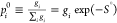, where g_i is the degeneracy factor of the ith outcome (likewise ). We then get that

9

S⁰ is the maximal value of S, which is obtained when the actual distribution, p_i, is equal to the prior distribution p_i⁰.⁶⁶ In other words, the prior distribution is the distribution of maximum entropy before taking into account the new constraints imposed by the data (beyond the degeneracy factors that always present and are inherent to the problem and were taken into account in the prior distribution). When the actual probability distribution is different than the prior distribution (owing to the additional constraints that became available from the experiments), the entropy is lower than S⁰. The term is the difference between the maximal and the actual value of the entropy and is therefore called the “entropy deficiency.”

In this paper, we maximized the information entropy (eq 9), which takes into account the prior distribution, p_i⁰, subject to the following three constrains.

• (1)
  All the probabilities are positive:

  
• (2)
  The probability distribution is normalized:

  
• (3)
  The average signal should fit the experimental scattering data:

  

where ϵ_q is defined by the noise level at each scattering angle. Note that the assumptions used to compute the prior distribution impose constraints (the constraints of the prior distribution will be discussed in the next section). It is convenient to solve the minimization problem for −S. The inequality constrained minimization problem can be solved by Lagrange multipliers method^68,69 (the full procedure is described in section 5 in the SI). The resultant distribution that maximizes the informational entropy subject to the constraint imposed by the data and our prior assumptions is given by

10

where

and λ is the vector of Lagrange multipliers (whose length is equal to the number of q points in the scattering curve), which sets the required probability distribution and was found by finding the solution to the Lagrange dual problem (as explain in section 5 in the SI) defined as

11

where

12

In this minimization problem, we can define a constraint to be active if λ_q ≠ 0 or inactive if λ_q = 0. Note that the last term in eq 12 can be interpreted as a form of L₁ regularization term, which promotes the sparsity of λ. Therefore, the minimization will result with the minimum number of active constraints, needed to satisfy all of the introduced constraints. As the values of ϵ increases, the sparsity of λ increases and hence the information content of the constraints decreases. The parameter vector ϵ is proportional to the noise level of the experimental signal, ϵ_q = βσ_q, where σ_q is the measured standard deviation of I_exp(q) and β is a global relaxation (or regularization) parameter. The Lagrange multiplier λ_q is related to the contribution of the added information from I_exp(q) and can therefore be used to estimate the information content of the signal by the number of active constraints in the entire measured q-range.

Thermodynamic Constraints

As we know additional chemical information on the problem, we can add additional constraints to the minimization problem. SAXS data alone contains limited information which may not necessarily overcome the overwhelming number of possible configurations, described by the degeneracies, g_i. Therefore, the additional chemical constraints confines the space of possibilities into a more realistic subspace that takes into consideration the stability of a given configuration. Common constraints for a self-assembly problem are given by the free energy gain in forming subunit–subunit interaction and a constraint regarding the expected mean number of dimers in an aggregate. Given these additional constraints, the new distribution is given by

13

where

14

The prior distribution, p_i^′0, is given by

15

where, ΔΩ_Gⁱ corresponds to the grand canonical free energy bias (for outcome i), which is a function of the free energy gain for creating interdimers bonds (see eq 6), E_i, and the free energy cost of taking n_i free subunits from the solution. The multipliers μ_E and μ_n are associated with the parameters and , respectively. Complete derivation of adding the thermodynamic prior is shown in section 5 in the SI.

Performing the Maximum Information Entropy Optimization on a Set of Time Series Data

Each time-resolved experiment was initiated by mixing a cold dimer solution with a concentrated ammonium acetate solution at 25 °C, resulting with a temperature and ionic strength jumps. The time evolution of an assembly reaction was given by the set of scattering intensities, {I(q, t_i)}, where t_i corresponds to the time interval between the mixing time and the time of the ith measurement and I(q, t_i) corresponds to the average scattering intensity during the 20 ms exposure of the measurement. To approximate the distribution of intermediates, p_n^s,c(t_i), we performed maximum entropy optimization (eq 11) on the entire series of signals, where i ∈ [1, .., m] and m is the number of measurement time points. If the assembly process is sampled at adequate frequency, the intermediate distributions, p_n(t), are likely to vary to a limited extent between consecutive measurements. The values of p_n^s,c(t_i) should continuously vary with time. As was discussed in our earlier paper,⁷⁰ when fitting a data series the continuity assumption may help to speed-up convergence.

To analyze our time-resolved data, we started the optimization from the first measured signal, I(q, t₁). As a prior distribution, we used the closest known result, which was the state of the protein solution before mixing with the salt solution. In this state, the interaction was weak and the protein was in its pure dimeric form (Figure 1a). The thermodynamic state of the system could be well describe by eq 15 with a weak association energy per contact of E_c = 5 k_BT and the total protein molar fraction X_total, determined by UV–vis adsorption measurement.

Following the optimization of the first time point, we have used the continuity of the probability distributions as a function of time. Hence, the prior distribution for the next signal, I(q, t₂), was the result of the optimization of the earlier time point (t₁). This extrapolation was applied until the last measurement (I(q, t_m)) was analyzed. Following the analysis of the last signal, the direction was reversed and the procedure continued in the same way from t_m backward to t₁. In this way, we minimized the effect of the assumed initial prior distribution, which was based on the state of the protein solution (before mixing with the salt solution).

To minimize the effect of the value of E_c on the prior distribution and thereby the results of the maximum entropy optimization, we performed an additional optimization set. In the second procedure we started from the latest measured time point, t_m, of the assembly reaction and used as a prior the thermodynamic probability distribution of the reaction products with an association free energy of E_c = 8.5 k_BT. This value was a result of our equilibrium measurement calibration of E_c, presented in Figure 2a). In this analysis, we assumed that the distribution in the latest time point, t_m, was not far removed from the equilibrium distribution. The same procedure was perform in the reversed order (from t₁ to t_m) and yielded similar results (p_n^s,c(t_i) values). Figures 3 and 4 present the average of the two procedures, and the error bars correspond to the deviations between the two sets of prior distributions (obtained with the two E_c values). The same two prior distributions were used for all the reactions conditions because even at high salt concentrations, the equilibrium SAXS data only slightly deviated from the thermodynamic model (Figure 1). Each assembly reaction was repeated between two and four times. The adequate fitting of the TR-SAXS data (Figure 3) confirms that our prior knowledge provided a good starting point for describing the assembly process.

Clustering of SAXS Models

Clustering of SAXS models, presented in Figure S22, was applied to the library of scattering models, used to analyze the static and time-resolved data. The full procedure was explained in our earlier work.³⁹ Briefly, we defined a weighted matrix, M, which included the set of m scattering models to be classified into clusters:Each column in the matrix contained a computed scattering intensity, I_i(q), with i ∈ [1, m]. The models were computed between q₁ = 0.1 nm^–1 and q_N = 1.1 nm^–1, the q range used for the time-resolved data analysis. The intensities were weighted according to the measured noise level, σⁱ(q_j), of the time-resolved measurements, where j ∈ [1, N]. The dimensions of the matrices were therefore N × m where N = 280 was the length of the model q⃗ vectors in the given q range, and m was 1361 and 749 for the T = 4 and T = 3 symmetries, respectively. The dimensions of the matrix were reduced using SVD analysis (eq 7). A k-means clustering algorithm⁷¹ was then applied to the reduced space. The number of clusters was defined as the minimal k that its χ² value given by

16

is smaller than 1 for all the models that were classified into the same cluster. Here, I_i(q_j) is a given model that was classified into cluster, c and I_c(q_j) is the modeled scattering intensity of the centroid of this cluster.

Limits of TR-SAXS Detection

Figure 4 shows sharp mass fraction peaks for T = 3 and T = 4 capsids, attributed to the thermodynamic prior (Figure S9), favoring stable complexes. It is important to note that TR-SAXS data are insufficient to distinguish between complete capsids and capsids that are missing few subunits, observed by CDMS.⁸ To take into consideration the limited sensitivity of TR-SAXS, we applied a clustering algorithm (Figure S22 in section 8 in the SI) to divide the configurational space into clusters that are likely to be indistinguishable by TR-SAXS (owing to its lower signal-to-noise ratio, compared with static SAXS data). With maximum broadening, particles missing six dimers may be included within the complete T = 4 peak. This broadening becomes wider with incomplete and degenerate particles (lower D_c values). Similar effects were observed for the T = 3 symmetry.

Intermediates containing 35 dimers or less could not be subclassified into T = 3 or T = 4 symmetries owing to the similarity in their scattering curves (Figure S23) and their low mass fraction. Within the signal-to-noise ratio of our data at the high q-range, the distinction between T = 3 and T = 4 particles is mostly limited to their different diameter. Therefore, the mass fraction at s = 90 may represent both well formed T = 3 particles and incomplete T = 3-like particles with s > 90 that deformed and assumed an average diameter, close to that of a T = 3, as suggested by CDMS experiments.⁸

Averaged Intermediate Size

The number-averaged size ⟨s⟩ of intermediates as a function of time, t, is given by

17

where s^–1X_n,s,c(t) is the molar fraction of T_n^s,c intermediate structures at time t.

Glossary

Abbreviations

HBV

hepatitis B virus

Cp

capsid protein

VLP

virus like particle

Cp149

149 residue assembly domain of HBV CP

SAXS

small-angle X-ray scattering

TR-SAXS

time-resolved SAXS

MC

Monte Carlo

CDMS

charge detection mass spectroscopy

SVD

singular value decomposition

Supporting Information Available

The Supporting Information is available free of charge at https://pubs.acs.org/doi/10.1021/jacs.0c01092.

• Static SAXS fitting using the thermodynamic model (complete set of SAXS fitting results; sensitivity analysis; equivalent measures of association free energy); additional results of slow time scale kinetics; comparing CDMS Results with SAXS Signals (demonstrating that at aggressive assembly conditions the radius of incomplete intermediates was smaller than the radius of a complete T = 4 capsid); details regarding SVD analysis for time-resolved data; complete derivation of maximum information entropy method including the thermodynamic constraints; results of maximum information entropy optimization (prior distributions; fitting results for reactions performed at 163, 313, and 513 mM ammonium acetate; sensitivity analysis in detecting small amounts of intermediates in TR-SAXS measurements with 163 mM ammonium acetate); observed D₁₀ intermediate, at 313 mM ammonium acetate, located at a local free energy minimum; results of clustering analysis of TR-SAXS signals (PDF)

The authors declare no competing financial interest.

References

- Cann A. In Principles of Molecular Virology, 5th ed.; Academic Press: London, 2012; pp 1–303. [Google Scholar]
- Caspar D. L.; Klug A. Physical principles in the construction of regular viruses. Cold Spring Harbor Symp. Quant. Biol. 1962, 27, 1–24. 10.1101/SQB.1962.027.001.005. [DOI] [PubMed] [Google Scholar]
- Panahandeh S.; Li S.; Marichal L.; Leite Rubim R.; Tresset G.; Zandi R. How a virus circumvents energy barriers to form symmetric shells. ACS Nano 2020, 14, 3170–3180. 10.1021/acsnano.9b08354. [DOI] [PubMed] [Google Scholar]
- Chevreuil M.; Law-Hine D.; Chen J.; Bressanelli S.; Combet S.; Constantin D.; Degrouard J.; Moller J.; Zeghal M.; Tresset G. Nonequilibrium self-assembly dynamics of icosahedral viral capsids packaging genome or polyelectrolyte. Nat. Commun. 2018, 9, 3071. 10.1038/s41467-018-05426-8. [DOI] [PMC free article] [PubMed] [Google Scholar]
- Waltmann C.; Asor R.; Raviv U.; Olvera de la Cruz M. Assembly and stability of simian virus 40 polymorphs. ACS Nano 2020, 10.1021/acsnano.9b10004. [DOI] [PMC free article] [PubMed] [Google Scholar]
- Kler S.; Asor R.; Li C.; Ginsburg A.; Harries D.; Oppenheim A.; Zlotnick A.; Raviv U. RNA encapsidation by SV40-derived nanoparticles follows a rapid two-state mechanism. J. Am. Chem. Soc. 2012, 134, 8823–8830. 10.1021/ja2110703. [DOI] [PMC free article] [PubMed] [Google Scholar]
- Chevreuil M.; Law-Hine D.; Chen J.; Bressanelli S.; Combet S.; Constantin D.; Degrouard J.; Möller J.; Zeghal M.; Tresset G. Nonequilibrium self-assembly dynamics of icosahedral viral capsids packaging genome or polyelectrolyte. Nat. Commun. 2018, 9, 3071. 10.1038/s41467-018-05426-8. [DOI] [PMC free article] [PubMed] [Google Scholar]
- Lutomski C. A.; Lyktey N. A.; Pierson E. E.; Zhao Z.; Zlotnick A.; Jarrold M. F. Multiple pathways in capsid assembly. J. Am. Chem. Soc. 2018, 140, 5784–5790. 10.1021/jacs.8b01804. [DOI] [PMC free article] [PubMed] [Google Scholar]
- Pierson E. E.; Keifer D. Z.; Selzer L.; Lee L. S.; Contino N. C.; Wang J. C.-Y.; Zlotnick A.; Jarrold M. F. Detection of late intermediates in virus capsid assembly by charge detection mass spectrometry. J. Am. Chem. Soc. 2014, 136, 3536–3541. 10.1021/ja411460w. [DOI] [PMC free article] [PubMed] [Google Scholar]
- Garmann R. F.; Comas-Garcia M.; Gopal A.; Knobler C. M.; Gelbart W. M. The assembly pathway of an icosahedral single-stranded RNA virus depends on the strength of inter-subunit attractions. J. Mol. Biol. 2014, 426, 1050–1060. 10.1016/j.jmb.2013.10.017. [DOI] [PMC free article] [PubMed] [Google Scholar]
- Perlmutter J. D.; Hagan M. F. Mechanisms of virus assembly. Annu. Rev. Phys. Chem. 2015, 66, 217. 10.1146/annurev-physchem-040214-121637. [DOI] [PMC free article] [PubMed] [Google Scholar]
- Hagan M. F.; Elrad O. M.; Jack R. L. Mechanisms of kinetic trapping in self-assembly and phase transformation. J. Chem. Phys. 2011, 135, 104115. 10.1063/1.3635775. [DOI] [PMC free article] [PubMed] [Google Scholar]
- Endres D.; Zlotnick A. Model-based analysis of assembly kinetics for virus capsids or other spherical polymers. Biophys. J. 2002, 83, 1217–1230. 10.1016/S0006-3495(02)75245-4. [DOI] [PMC free article] [PubMed] [Google Scholar]
- Tresset G.; Le Coeur C.; Bryche J.-F.; Tatou M.; Zeghal M.; Charpilienne A.; Poncet D.; Constantin D.; Bressanelli S. Norovirus capsid proteins self-assemble through biphasic kinetics via long-lived stave-like intermediates. J. Am. Chem. Soc. 2013, 135, 15373–15381. 10.1021/ja403550f. [DOI] [PubMed] [Google Scholar]
- Garmann R. F.; Goldfain A. M.; Manoharan V. N. Measurements of the self-assembly kinetics of individual viral capsids around their RNA genome. Proc. Natl. Acad. Sci. U. S. A. 2019, 116, 22485–22490. 10.1073/pnas.1909223116. [DOI] [PMC free article] [PubMed] [Google Scholar]
- Borodavka A.; Tuma R.; Stockley P. G. Evidence that viral RNAs have evolved for efficient, two-stage packaging. Proc. Natl. Acad. Sci. U. S. A. 2012, 109, 15769–15774. 10.1073/pnas.1204357109. [DOI] [PMC free article] [PubMed] [Google Scholar]
- Marchetti M.; Kamsma D.; Cazares Vargas E.; Hernandez García A.; van der Schoot P.; de Vries R.; Wuite G. J. L.; Roos W. H. Real-time assembly of viruslike nucleocapsids elucidated at the single-particle level. Nano Lett. 2019, 19, 5746–5753. 10.1021/acs.nanolett.9b02376. [DOI] [PMC free article] [PubMed] [Google Scholar]
- Asor R.; Khaykelson D.; Ben-nun Shaul O.; Levi-Kalisman Y.; Oppenheim A.; Raviv U. pH stability and disassembly mechanism of wild-type simian virus 40. Soft Matter 2020, 16, 2803–2814. 10.1039/C9SM02436K. [DOI] [PMC free article] [PubMed] [Google Scholar]
- Zlotnick A. Are weak protein–protein interactions the general rule in capsid assembly?. Virology 2003, 315, 269–274. 10.1016/S0042-6822(03)00586-5. [DOI] [PubMed] [Google Scholar]
- Rapaport D. Molecular dynamics study of T= 3 capsid assembly. J. Biol. Phys. 2018, 44, 147–162. 10.1007/s10867-018-9486-7. [DOI] [PMC free article] [PubMed] [Google Scholar]
- Schwartz R.; Shor P. W.; Prevelige P. E.; Berger B. Local rules simulation of the kinetics of virus capsid self-assembly. Biophys. J. 1998, 75, 2626–2636. 10.1016/S0006-3495(98)77708-2. [DOI] [PMC free article] [PubMed] [Google Scholar]
- Rapaport D. Role of reversibility in viral capsid growth: a paradigm for self-assembly. Phys. Rev. Lett. 2008, 101, 186101. 10.1103/PhysRevLett.101.186101. [DOI] [PubMed] [Google Scholar]
- Zandi R.; van der Schoot P.; Reguera D.; Kegel W.; Reiss H. Classical nucleation theory of virus capsids. Biophys. J. 2006, 90, 1939–1948. 10.1529/biophysj.105.072975. [DOI] [PMC free article] [PubMed] [Google Scholar]
- Nguyen H. D.; Reddy V. S.; Brooks C. L. Deciphering the kinetic mechanism of spontaneous self-assembly of icosahedral capsids. Nano Lett. 2007, 7, 338–344. 10.1021/nl062449h. [DOI] [PubMed] [Google Scholar]
- Oosawa F.; Asakura S.. Thermodynamics of the Polymerization of Protein; Academic Press: London, 1975. [Google Scholar]
- Razavi-Shearer D.; et al. Global prevalence, treatment, and prevention of hepatitis B virus infection in 2016: a modelling study. Lancet Gastroenterology and Hepatology 2018, 3, 383–403. 10.1016/S2468-1253(18)30056-6. [DOI] [PubMed] [Google Scholar]
- Venkatakrishnan B.; Zlotnick A. The structural biology of hepatitis B virus: form and function. Annu. Rev. Virol. 2016, 3, 429–451. 10.1146/annurev-virology-110615-042238. [DOI] [PMC free article] [PubMed] [Google Scholar]
- Ning X.; Nguyen D.; Mentzer L.; Adams C.; Lee H.; Ashley R.; Hafenstein S.; Hu J. Secretion of genome-free hepatitis B virus–single strand blocking model for virion morphogenesis of para-retrovirus. PLoS Pathog. 2011, 7, e1002255. 10.1371/journal.ppat.1002255. [DOI] [PMC free article] [PubMed] [Google Scholar]
- Seeger C.; Mason W. S. Molecular biology of hepatitis B virus infection. Virology 2015, 479, 672–686. 10.1016/j.virol.2015.02.031. [DOI] [PMC free article] [PubMed] [Google Scholar]
- Patel N.; White S. J.; Thompson R. F.; Bingham R.; Weiß E. U.; Maskell D. P.; Zlotnick A.; Dykeman E. C.; Tuma R.; Twarock R.; Ranson N. A.; Stockley P. G. HBV RNA pre-genome encodes specific motifs that mediate interactions with the viral core protein that promote nucleocapsid assembly. Nat. Microbiol. 2017, 2, 17098. 10.1038/nmicrobiol.2017.98. [DOI] [PMC free article] [PubMed] [Google Scholar]
- Stray S. J.; Bourne C. R.; Punna S.; Lewis W. G.; Finn M. G.; Zlotnick A. A heteroaryldihydropyrimidine activates and can misdirect hepatitis B virus capsid assembly. Proc. Natl. Acad. Sci. U. S. A. 2005, 102, 8138–8143. 10.1073/pnas.0409732102. [DOI] [PMC free article] [PubMed] [Google Scholar]
- Kondylis P.; Schlicksup C. J.; Brunk N. E.; Zhou J.; Zlotnick A.; Jacobson S. C. Competition between normative and drug-induced virus self-assembly observed with single-particle methods. J. Am. Chem. Soc. 2019, 141, 1251–1260. 10.1021/jacs.8b10131. [DOI] [PMC free article] [PubMed] [Google Scholar]
- Yuen M.-F.; Agarwal K.; Gane E. J.; Schwabe C.; Ahn S. H.; Kim D. J.; Lim Y.-S.; Cheng W.; Sievert W.; Visvanathan K.; Ruby E.; Liaw S.; Yan R.; Connelly E.; Cai D.; Huang Q.; Colonno R.; Lopatin U. A.. Final results of a phase 1b 28-day study of ABI-H0731, a novel core inhibitor, in non-cirrhotic viremic subjects with chronic hepatitis B. Annual Meeting of the American Association for the Study of Liver-Diseases (AASLD)/Liver Meeting, San Francisco, CA, November 9–13, 2018
- Wang J. C.-Y.; Nickens D. G.; Lentz T. B.; Loeb D. D.; Zlotnick A. Encapsidated hepatitis B virus reverse transcriptase is poised on an ordered RNA lattice. Proc. Natl. Acad. Sci. U. S. A. 2014, 111, 11329–11334. 10.1073/pnas.1321424111. [DOI] [PMC free article] [PubMed] [Google Scholar]
- Packianathan C.; Katen S. P.; Dann C. E.; Zlotnick A. Conformational changes in the hepatitis B virus core protein are consistent with a role for allostery in virus assembly. J. Virol. 2010, 84, 1607–1615. 10.1128/JVI.02033-09. [DOI] [PMC free article] [PubMed] [Google Scholar]
- Zhao Z.; Wang J. C.-Y.; Gonzalez-Gutierrez G.; Venkatakrishnan B.; Asor R.; Khaykelson D.; Raviv U.; Zlotnick A. Structural differences between the woodchuck hepatitis virus core protein in the dimer and capsid states are consistent with entropic and conformational regulation of assembly. J. Virol. 2019, 93, e00141-19. 10.1128/JVI.00141-19. [DOI] [PMC free article] [PubMed] [Google Scholar]
- Wynne S.; Crowther R.; Leslie A. The crystal structure of the human hepatitis B virus capsid. Mol. Cell 1999, 3, 771–780. 10.1016/S1097-2765(01)80009-5. [DOI] [PubMed] [Google Scholar]
- Ceres P.; Zlotnick A. Weak protein- protein interactions are sufficient to drive assembly of hepatitis B virus capsids. Biochemistry 2002, 41, 11525–11531. 10.1021/bi0261645. [DOI] [PubMed] [Google Scholar]
- Asor R.; Selzer L.; Schlicksup C. J.; Zhao Z.; Zlotnick A.; Raviv U. Assembly reactions of hepatitis B capsid protein into capsid nanoparticles follow a narrow path through a complex reaction landscape. ACS Nano 2019, 13, 7610–7626. 10.1021/acsnano.9b00648. [DOI] [PMC free article] [PubMed] [Google Scholar]
- Kegel W. K.; van der Schoot P. Competing hydrophobic and screened-coulomb interactions in hepatitis B virus capsid assembly. Biophys. J. 2004, 86, 3905–3913. 10.1529/biophysj.104.040055. [DOI] [PMC free article] [PubMed] [Google Scholar]
- Harms Z. D.; Selzer L.; Zlotnick A.; Jacobson S. C. Monitoring assembly of virus capsids with nanofluidic devices. ACS Nano 2015, 9, 9087–9096. 10.1021/acsnano.5b03231. [DOI] [PMC free article] [PubMed] [Google Scholar]
- Ben-Shaul A.; Gelbart W. M.. Statistical thermodynamics of amphiphile self-assembly: structure and phase transitions in micellar solutions. In Micelles, Membranes, Microemulsions, and Monolayers; Gelbart W. M., Ben-Shaul A., Roux D., Eds.; Springer: New York, 1994; pp 1–104. [Google Scholar]
- Moisant P.; Neeman H.; Zlotnick A. Exploring the paths of (virus) assembly. Biophys. J. 2010, 99, 1350–1357. 10.1016/j.bpj.2010.06.030. [DOI] [PMC free article] [PubMed] [Google Scholar]
- Zlotnick A.; Johnson J. M.; Wingfield P. W.; Stahl S. J.; Endres D. A theoretical model successfully identifies features of hepatitis B virus capsid assembly. Biochemistry 1999, 38, 14644–14652. 10.1021/bi991611a. [DOI] [PubMed] [Google Scholar]
- Lutomski C. A.; Lyktey N. A.; Zhao Z.; Pierson E. E.; Zlotnick A.; Jarrold M. F. Hepatitis B virus capsid completion occurs through error correction. J. Am. Chem. Soc. 2017, 139, 16932–16938. 10.1021/jacs.7b09932. [DOI] [PMC free article] [PubMed] [Google Scholar]
- Zhou J.; Kondylis P.; Haywood D. G.; Harms Z. D.; Lee L. S.; Zlotnick A.; Jacobson S. C. Characterization of virus capsids and their assembly intermediates by multicycle resistive-pulse sensing with four pores in series. Anal. Chem. 2018, 90, 7267–7274. 10.1021/acs.analchem.8b00452. [DOI] [PMC free article] [PubMed] [Google Scholar]
- Khaykelson D.; Raviv U. Studying viruses using solution X-ray scattering. Biophys. Rev. 2020, 12, 41–48. 10.1007/s12551-020-00617-4. [DOI] [PMC free article] [PubMed] [Google Scholar]
- Ginsburg A.; Ben-Nun T.; Asor R.; Shemesh A.; Ringel I.; Raviv U. Reciprocal grids: a hierarchical algorithm for computing solution X-ray scattering curves from supramolecular complexes at high resolution. J. Chem. Inf. Model. 2016, 56, 1518. 10.1021/acs.jcim.6b00159. [DOI] [PubMed] [Google Scholar]
- Ginsburg A.; Ben-Nun T.; Asor R.; Shemesh A.; Fink L.; Tekoah R.; Levartovsky Y.; Khaykelson D.; Dharan R.; Fellig A.; Raviv U. D+: software for high-resolution hierarchical modeling of solution X-ray scattering from complex structures. J. Appl. Crystallogr. 2019, 52, 219–242. 10.1107/S1600576718018046. [DOI] [PMC free article] [PubMed] [Google Scholar]
- Zlotnick A. To build a virus capsid: an equilibrium model of the self assembly of polyhedral protein complexes. J. Mol. Biol. 1994, 241, 59–67. 10.1006/jmbi.1994.1473. [DOI] [PubMed] [Google Scholar]
- Endres D.; Miyahara M.; Moisant P.; Zlotnick A. A reaction landscape identifies the intermediates critical for self-assembly of virus capsids and other polyhedral structures. Protein Sci. 2005, 14, 1518–1525. 10.1110/ps.041314405. [DOI] [PMC free article] [PubMed] [Google Scholar]
- Henry E.; Hofrichter J.. Singular value decomposition: Application to analysis of experimental data. In Numerical Computer Methods; Methods in Enzymology; Academic Press, 1992; Vol. 210, pp 129–192. [Google Scholar]
- Hagan M. F.; Elrad O. M. Understanding the concentration dependence of viral capsid assembly kinetics–the origin of the lag time and identifying the critical nucleus size. Biophys. J. 2010, 98, 1065–1074. 10.1016/j.bpj.2009.11.023. [DOI] [PMC free article] [PubMed] [Google Scholar]
- Rapaport D. C. Self-assembly of polyhedral shells: A molecular dynamics study. Phys. Rev. E 2004, 70, 051905. 10.1103/PhysRevE.70.051905. [DOI] [PubMed] [Google Scholar]
- Zlotnick A.; Ceres P.; Singh S.; Johnson J. M. A small molecule inhibits and misdirects assembly of hepatitis B virus capsids. J. Virol. 2002, 76, 4848–4854. 10.1128/JVI.76.10.4848-4854.2002. [DOI] [PMC free article] [PubMed] [Google Scholar]
- Blanchet C. E.; Spilotros A.; Schwemmer F.; Graewert M. A.; Kikhney A.; Jeffries C. M.; Franke D.; Mark D.; Zengerle R.; Cipriani F.; Fiedler S.; Roessle M.; Svergun D. I. Versatile sample environments and automation for biological solution X-ray scattering experiments at the P12 beamline (PETRA III, DESY). J. Appl. Crystallogr. 2015, 48, 431–443. 10.1107/S160057671500254X. [DOI] [PMC free article] [PubMed] [Google Scholar]
- Round A.; Felisaz F.; Fodinger L.; Gobbo A.; Huet J.; Villard C.; Blanchet C. E.; Pernot P.; McSweeney S.; Roessle M.; Svergun D. I.; Cipriani F. BioSAXS sample changer: a robotic sample changer for rapid and reliable high-throughput X-ray solution scattering experiments. Acta Crystallogr., Sect. D: Biol. Crystallogr. 2015, 71, 67–75. 10.1107/S1399004714026959. [DOI] [PMC free article] [PubMed] [Google Scholar]
- Hammersley A. FIT2D: a multi-purpose data reduction, analysis and visualization program. J. Appl. Crystallogr. 2016, 49, 646. 10.1107/S1600576716000455. [DOI] [Google Scholar]
- Asor R.; Ben-nun Shaul O.; Oppenheim A.; Raviv U. Crystallization, reentrant melting, and resolubilization of virus nanoparticles. ACS Nano 2017, 11, 9814–9824. 10.1021/acsnano.7b03131. [DOI] [PMC free article] [PubMed] [Google Scholar]
- Ginsburg A.; Shemesh A.; Millgram A.; Dharan R.; Levi-Kalisman Y.; Ringel I.; Raviv U. Structure of dynamic, taxol-stabilized, and GMPPCP-stabilized microtubule. J. Phys. Chem. B 2017, 121, 8427–8436. 10.1021/acs.jpcb.7b01057. [DOI] [PubMed] [Google Scholar]
- Asor R.; Khaykelson D.; Ben-nun Shaul O.; Oppenheim A.; Raviv U. Effect of calcium ions and disulfide bonds on swelling of virus particles. ACS Omega 2019, 4, 58–64. 10.1021/acsomega.8b02753. [DOI] [PMC free article] [PubMed] [Google Scholar]
- Van Vaerenbergh P.; Léonardon J.; Sztucki M.; Boesecke P.; Gorini J.; Claustre L.; Sever F.; Morse J.; Narayanan T.. An upgrade beamline for combined wide, small and ultra small-angle x-ray scattering at the ESRF. Proceedings of the 12th International Conference on Synchrotron Radiation Instrumentation (SRI2015), New York, July 6–10, 2015, 2016; p 030034.
- Narayanan T.; Sztucki M.; Van Vaerenbergh P.; Léonardon J.; Gorini J.; Claustre L.; Sever F.; Morse J.; Boesecke P. A multipurpose instrument for time-resolved ultra-small-angle and coherent X-ray scattering. J. Appl. Crystallogr. 2018, 51, 1511–1524. 10.1107/S1600576718012748. [DOI] [PMC free article] [PubMed] [Google Scholar]
- Saper G.; Kler S.; Asor R.; Oppenheim A.; Raviv U.; Harries D. Effect of capsid confinement on the chromatin organization of the SV40 minichromosome. Nucleic Acids Res. 2013, 41, 1569–1580. 10.1093/nar/gks1270. [DOI] [PMC free article] [PubMed] [Google Scholar]
- Jaynes E. T. Information theory and statistical mechanics. Phys. Rev. 1957, 106, 620. 10.1103/PhysRev.106.620. [DOI] [Google Scholar]
- Levine R. D. An information theoretical approach to inversion problems. J. Phys. A: Math. Gen. 1980, 13, 91. 10.1088/0305-4470/13/1/011. [DOI] [Google Scholar]
- Shannon C. E. A mathematical theory of communication (parts I and II). Bell Syst. Tech. J. 1948, 27, 379–423. 10.1002/j.1538-7305.1948.tb01338.x. [DOI] [Google Scholar]
- Kazama J.; Tsujii J. Maximum entropy models with inequality constraints: A case study on text categorization. Machine Learning 2005, 60, 159–194. 10.1007/s10994-005-0911-3. [DOI] [Google Scholar]
- Boyd S.; Vandenberghe L.. Convex Optimization; Cambridge University Press, 2004. [Google Scholar]
- Ben-Nun T.; Barak A.; Raviv U. Spline-based parallel nonlinear optimization of function sequences. J. Parallel Distr. Com. 2016, 93, 132–145. 10.1016/j.jpdc.2016.04.011. [DOI] [Google Scholar]
- MacQueen J.Some methods for classification and analysis of multivariate observations. Proceedings of the Fifth Berkeley Symposium on Mathematical Statistics and Probability, Berkeley, California, 1967; pp 281–297.
Associated Data
This section collects any data citations, data availability statements, or supplementary materials included in this article.