

Abstract
For many viruses, capsids (biological nanoparticles) assemble to protect genetic material and dissociate to release their cargo. To understand these contradictory properties, we analyzed capsid assembly for Hepatitis B virus; an endemic pathogen with an icosahedral, 120-homodimer capsid. We used solution X-ray scattering to examine trapped and equilibrated assembly reactions. To fit experimental results, we generated a library of unique intermediates, selected by umbrella sampling of Monte Carlo simulations. The number of possible capsid intermediates is immense, ~ 1030, yet assembly reactions are rapid and completed with high fidelity. If the huge number of possible intermediates were actually present, maximum entropy analysis shows that assembly reactions would be blocked by an entropic barrier, resulting in incomplete nanoparticles. When an energetic term was applied to select the stable species that dominated the reaction mixture, we found that only a few hundred intermediates, mapping out a narrow path through the immense reaction landscape. This is a solution to a viral application of the Levinthal paradox. With the correct energetic term, the match between predicted intermediates and scattering data was striking. The grand canonical free energy landscape for assembly, calibrated by our experimental results, supports a detailed analysis of this complex reaction. There is a narrow range of energies that supports on-path assembly. If association energy is too weak or too strong progressively more intermediates will be entropically blocked, spilling into paths leading to dissociation or trapped incomplete nanoparticles, respectively. These results are relevant to many viruses, provide a basis for simplifying assembly models and identifying new targets for antiviral intervention. They provide a basis for understanding and designing biological and abiological self-assembly reactions.
Graphical Abstract
Introduction
Large macromolecular complexes are ubiquitous in nature, yet the assembly paths that lead to thermodynamically stable products have rarely been determined. A challenging example is the assembly of viral capsids (biological nanoparticles). In about half of known virus families, the capsid is a spherical/icosahedral protein complex. Depending on the virus, capsids may package nucleic acid during assembly and/or remain empty, typically as a Trojan horse, a storage form, or an immature particle for subsequent nucleic acid packaging. In many cases, purified capsid protein (CP) molecules can be induced to spontaneously assemble into viruslike capsids. Paradoxically, capsids that protect their genome can be induced to dissociate to release their genetic cargo. The interactions between CP subunits should therefore support the formation of both stable yet dynamic capsid structures.1-5
To understand this reaction, many groups have examined assembly in vitro.6-8 The simplest case is where CP subunits at suitable buffer conditions, assemble into empty capsids by a nucleation-elongation mechanism.9-11 Virus-like particles (VLPs) can also form around synthetic polymers, RNA, or DNA.12-17 From materials perspective, understanding the thermodynamic stability of virus capsid nanoparticles or VLPs is of great interest owing to their potential use in bionanomedical and bionanomaterial applications.18 VLPs may serve as protein nanocapsules, nanocarriers for nanoparticles, drug or gene delivery vehicles, biosensors, scaffolds for display of antigens for vaccine applications, or as nanoreactors for catalysis.19-25
In vivo, the nucleoprotein core of Hepatitis B virus (HBV) assembles in the cytoplasm from 120 CP dimers, either as empty nanoparticles or while packaging viral RNA and viral reverse transcriptase. The reverse transcriptase becomes active after assembly, synthesizing a circular dsDNA genome from the linear ssRNA "pregenome" within the T = 4 icosahedral capsid (Figure 1). The mature DNA-filled core (and empty cores) can then be secreted from a cell while acquiring a protein and lipid envelope. In vitro, the dimers of the 149 residue assembly domain (cp149) can be driven to assemble into virus like capsids by increasing ionic strength, reaction temperature, and cp149 concentration.1-3,26 In vitro and in vivo,27 there is a small population of T = 3 nanoparticles composed of dimers (Figure 1). This assembly reaction has been characterized, under a wide range of conditions. The results showed that cp149 protein is a well behaved and tractable model system.1-4 More recently, mass spectrometry and nanofluidic resistive-pulse sensing have provided improved single particle and temporal resolution to study intermediates and capsids formation along the assembly pathway.7,8,28,29
Figure 1:

Atomic model (red and green) and graph representation (blue) of T = 3 (left) and T = 4 (right) icosahedral capsid symmetries. Each vertex of the graph is at the geometric center of a dimer subunit whereas each edge corresponded to a contact between adjacent dimers. Red and green colors represent the two dimer positions. The three types of interactions (the edges of the graph) are indicated by white letters. T is the triangulation number, defined as the square of the distance between two adjacent five-fold vertices. 60T is the number of monomer subunits comprising the icosahedral structure. T = 3 contains 90 dimers (180 monomers) and T = 4 has 120 dimers (240 monomers). The outer diameters of T = 3 and T = 4 are 28 and 32 nm, respectively.
To attain a comprehensive description of the ensemble of species in HBV capsid assembly reactions, we have collected solution small-angle X-ray scattering (SAXS) data and deconvolved them to a library of model structures derived from umbrella sampling Monte Carlo (MC) simulations of assembly. Using our home-developed software, D+ (https://scholars.huji.ac.il/uriraviv/software/d-software),30,31 we computed the solution scattering curve contribution from the atomic model of each intermediate. Because of the extraordinary number of possible intermediates, unrestrained selections of intermediates using a maximum entropy approach,32,33 yielded a chemically and experimentally unrealistic result, a recapitulation of the Levinthal paradox.34 By incorporating thermodynamic constraints on the assembly reaction we dramatically restricted the number of products and obtained compelling interpretations of the data.
We found that a narrow range of dimer-dimer association free energy led to assembly without intermediates. Under those conditions, the path of minimum grand canonical free energy starts at the reactants and ends at the final global minimum energy products, passing through a downhill energy landscape with minimal potential for pathways that could lead to out-of-equilibrium metastable, kinetically trapped intermediates. Under- or over-shooting the ideal energy opened up reaction pathways that led to progressively more kinetically trapped intermediates.
Results and Discussion
Determining capsid assembly reaction products
At low temperature and low ionic strength, cp149 is exclusively dimer
The initial state of the capsid protein solution is critical for the study of its assembly process. Partial assemblies and nonspecific aggregates are likely to affect the assembly path or yield. Figure 2 shows the absolute scattering intensity curve (see Section 1a in the supporting information, SI) from the initial capsid protein solution. Using D+ software (https://scholars.huji.ac.il/uriraviv/software/d-software),30,31 the curve was fitted to the atomic model of a solvated capsid protein dimeric subunit, where the electron density and the thickness of the hydration shell were fitted to the scattering data. The excellent agreement with the calculated intensity indicates that the initial state for the assembly reaction was pure cp149 dimer. Within the limited resolution of the SAXS curve (about 1nm), the conformation of the dimer in its soluble state was similar to its conformation in the capsid. Significant conformational differences between the free dimer and capsid states are still possible.35 The structure of the solvated dimer, used for fitting the data in Figure 2, measured at 9 °C, was used as the basic subunit to construct the entire intermediates configurational space, used later for fitting the data at all the temperatures. Additionally, we used these data to set the hydration layer parameters of all the other intermediate structural models, eliminating the need to fit additional parameters in the subsequent structural analyses. The assumption in this approximation was that in the intermediate assemblies, the contribution to the scattering intensity from the overlap between the hydration shells of the dimers was negligible. This assumption was validated by verifying that the computed scattering curve from the hydrated capsid was similar to the curve of a capsid that was computed from hydrated dimers (see Figure S1 and Section 1b in the SI).
Figure 2:

Cp149 is dimeric. Azimuthally integrated background-subtracted absolute small angle X-ray scattering intensity (see Section 1a in the SI) from 25 μM (0.9 ) cp149, at 50mM HEPES, pH 7.5, at 9 °C (blue symbols) fit to a hydrated model dimer (red line). Aggregates were avoided by applying the protocol explained in Sample Preparation in Materials and Methods. Measurement error bars are shown in gray. The modeled intensity was calculated using the atomic coordinates of cp149 dimer (PDB ID 2G33). Hydrogen atoms were added to the PDB file using MolProbity server36 and the hydration layer was fitted using D+ software. The best fitted values for the thickness and electron density of the hydration layer were 2 Å and 363 , respectively.
The NaCl concentration for the formation of capsids decreases with temperature
SAXS data recapitulated ionic strength and temperature dependence of assembly observed in earlier studies1,2,4,8,26,37,38 but provided new insights. Assembly of 20 μM cp149 was initiated by mixing 25 μM cp149 in 50mM HEPES at pH 7.5 with a concentrated buffered NaCl solution, to final NaCl concentrations between 0 and 1 M, in 50 mM HEPES at pH 7.5. Figure 3 shows the scattering intensity curves measured after several hours of incubation. At 9 or 25 °C, 300 mM NaCl were needed to form capsids. At 36 °C, capsid-like particles were already evident at 50 mM NaCl.
Figure 3:

Equilibrated or trapped cp149 assembly reactions at different temperatures and NaCl concentrations. The figure shows the background-subtracted signals (blue symbols), the standard deviations (gray bars), and fitted models (red curves). The modeling of each curve was done by fixing the total protein concentration to the experimental value and fitting the interdimer association free energy for T = 4 capsids and the relative association energy for T = 3 capsid (Equation 26 and 27). The 9 °C panel presents the atomic structure of cp149 dimer (bottom left) and T = 4 capsid (upper right), not at the same scale. The values of the best fitted interdimer association free energies are provided in Figure 7 and Table S1.
Enumeration of the "en-route" intermediate sample space during the assembly process
To analyze SAXS data for an assembly reaction where there are likely to be a broad ensemble of intermediates, we created an appropriate series of models. is an icosahedral capsid or intermediate, whose triangulation number is n, and is made of s capsid protein dimer subunits, held together by c dimer-dimer contacts. An intact T = 4 particle would be . A SAXS curve is influenced by both the size and the shape of the objects that contribute to the scattering intensity as well as by the distribution of the total protein mass between these objects (see Section 1d in the SI). In this enumeration the size and shape depend on s, c, and the manner by which the assembled dimers are connected to each other. There may be many different arrangements of subunits that match a given s,c index.
To construct the sample space of the possible "en-route" capsid intermediates, we examined the configuration space in the s-c plane. The configuration space includes information about the range of possible intermediates (with c values between cmin (s) and cmax (s) for each intermediate size, s), and about the degeneracy for each intermediate type (see Materials and Methods). Once the configuration space is defined, the probability of finding a specific structure for a given experimental condition can be estimated from the relevant partition function. Figure 4a shows the distribution of states (Ω4,s,c) of T = 4 intermediates based on MC simulation where the sampling was not biased by the stability of intermediates (see Materials and Methods). T = 4 and T = 3 configurations had similar distributions of intermediates with a peak in heterogeneity above the midpoint in size (Figures S9 and S10 and Sections 2a and 2b in the SI). A similar distribution was seen for smaller geometric figures (Figure S13 and Section 2d in the SI).4 Note that the distribution is asymmetric, with a peak when ≈ of the capsid is complete (Figure S10), because only connected structures were allowed. As the occupancy increased, the connectivity constraint excluded fewer states and shifted the maximum number of allowed intermediates towards larger sizes. Viewed from a different perspective, large intermediates have a broad range of holes.4
Figure 4:

The distribution of states for intermediates as a function of intermediate size (s) and number of dimer-dimer contacts (c), based on umbrella-sampled MC simulations. (a) 2D sampling assuming zero free energy per contact. The colors and contours represent the number of different configurations, Ω4,s,c, for particles with a given c and s values. (b) The same distribution of states from (a) as a function of size (s) and degree of connectivity, DC (Eq. 1). The color-scale is logarithmic. (c) 1D distribution of 76-dimer intermediates based on zero energy simulation. (d) The relative probability of intermediates with respect to the lowest energy intermediate when Boltzmann’s factor was introduced for the case where the association free energy was set to −7 kBT.
Figure 4b maps the distribution of states from the c − s plane to the DC − s plane, where
| (1) |
is the degree of connectivity. In this representation the most compact structures (highest degree of connectivity) are along the DC(s) = 1 line and the structures with the lowest degree of connectivity are found along the DC(s) = 0 line. The dimer and full capsid were placed at (s, DC) = (1, 1) and (s, DC) = (120, 1), respectively.
Most intermediate states were based on extended strings of subunits or had many holes (DC ≃ 0.3). The states with the smallest number of configurations corresponds to the most compact structures, which also have the maximal number of contacts for a given size (and minimal number of holes). This is demonstrated in Figure 4c for intermediates of size 76, which pass through the peak of the distribution. The total number of possible states, Ωtotal = Σn Σs Σc Ωn,s,c, based on simulations, was ≃ 1.82 × 1030. The distribution of states sampled by our MC simulation provides new information on the configurational degeneracy of the capsid assembly process.
The zero energy probabilities alone, however, were insufficient to determine the composition of intermediates of the assembly reaction at equilibrium. Attempts to fit SAXS data using a maximum entropy approach, leading to the broadest intermediate distribution that the scattering data do not exclude,32,33 failed because of the overwhelming number of incomplete capsids states whose calculated scattering curves are similar to that of a T = 4 particle (see Figures S2-S4 and Section 1c in the SI for a discussion about maximum entropy analysis). A fit with this nonrepresentative library suggests a large concentration of incomplete intermediates, contrary to experimental observations by charge detection mass spectrometry and nanofluidic resistive-pulse sensing,8,28,29 which showed that T = 4 capsid is the major reaction product in mild assembly conditions. The unedited library is essentially the Levinthal prediction that the number of possible intermediates is so great that only a small fraction can reasonably be sampled.34 In retrospect, the unedited library of intermediates requires the unrealistic assumption that all intermediates are equally accessible. A more rigorous weighting of the library is based on the complete grand canonical partition function, which describes the thermodynamics of macromolecular self-assembly processes. The important caveat of this weighting is that it assumes reactions are approximately equilibrated.
Figure 4d demonstrates the effect of including a bias to the distribution of intermediates of size 76 based on the association free energy. At equilibrium, when the association free energy is included, the conformational space is confined to intermediates with the highest degree of connectivity. For the 76-mers, intermediates with <140 contacts are predicted to make a negligible contribution to the reaction products. The incorporation of association energy into the thermodynamic model (the exponential term in Equation 2), reduces the number of intermediates used to model the reaction products to a few hundreds.
Experimental SAXS data show excellent agreement with the thermodynamic analysis
Making the assumption that intermediates are limited to about 1030 on-path structures, we can determine the association energy for T = 4 and T = 3 capsids by obtaining the best fit of the Boltzmann weighting factor to the observed distribution of species. The two free energies per contact, ΔF4 and ΔF3, for the T = 4 and T = 3 capsid symmetries, respectively, are the only adjustable terms in the equation. In practical terms, minimizing the total free energy of the grand canonical ensemble (see Equation 16 in Materials and Methods) yielded the molar fraction of dimer subunits, Xn,s,c, in each of the possible intermediate structures in the configurational space:
| (2) |
Equation 2 (derived in Materials and Methods) shows that the total mole fraction of protein in each intermediate, Xn,s,c, is a function of (i) the configurational entropy term, kBT ln Ωn,s,c, determined from our MC simulations, (ii) the chemical potential of free dimer μ1, set by the total protein concentration and the law of mass conservation, and (iii) the two free energies per contact, ΔF4 and ΔF3. As previously noted, s is the number of dimeric subunits, c is the number of dimer-dimer contacts, and kBT is Boltzmann’s constant multiplied by the absolute temperature.
Figure 3 shows the experimental and the fitted scattering intensity models (see Equation 26 in Materials and Methods) for the data set measured at a protein concentration of 20 μM. The results show remarkable agreement with the thermodynamic model throughout the entire range of conditions and scattering angles. Small deviations from the model were only observed under extreme experimental conditions and can be seen at the low q range (NaCl concentration of 0.5 M or higher; and temperature of 25 °C or higher; see Figure S14 and Section 3 in the SI).
Figure 5 maps the temperature - NaCl concentration phase space at 20 μM cp149, based on the level of agreement in Figure 3 between the data and our thermodynamic model. At high salt and temperature, deviations were classified into two groups according to difference between the data and the best fitted model. Nonetheless, under a broad range of conditions, the thermodynamic model provided an excellent prediction to the composition of the capsid assembly reaction products at equilibrium. The quality of the fit indicates that the most observed intermediates closely resembled fragments of T = 4 and T = 3 capsids with appropriate radii of curvature; only under extreme conditions a small fraction of off-path and/or aggregated products accumulated. Figures S20 - S22 suggest that using slow dialysis, the boarders (broken curves) in Figure 5 could have been extended to somewhat higher salt concentrations and temperatures.38
Figure 5:

Mapping the temperature - NaCl concentration phase space of capsid assembly at 20 μM cp149, based on the degree of agreement between our experiments and thermodynamic model. Each symbol in the phase diagram represents an assembly reaction, classified according to its level of agreement with the thermodynamic model (presented in Figures 3 and S14): excellent agreement (blue), very small deviations (orange), and small deviations (red). Note that physiological ionic strength and temperature are predicted to yield equilibrated reactions. Red and orange qualitative broken contours were added to visually separate the three phases. Figure S15 shows the χ2 values of the fitted SAXS models in Figure 3, based on which the fitting quality was classified.
At equilibrium, our thermodynamic analysis predicts that the main products of our assembly reactions were dimer subunits and full capsids (Figure 6). Large intermediates were not present at detectable concentrations. Throughout the data set, more than 99% of the protein mass was found as dimer and full capsids. Most of the rest of the protein mass comprised tetramers (dimers of dimers) and hexamers (trimers of dimers). The mass fractions of other intermediate structures were lower than the detection limit in our SAXS measurements and modeling (see Sections 1d and 1e in the SI). At high ionic strength the major assembly product was T = 4 capsid. The entire data set followed a universal curve (Figure 6d).39
Figure 6:

Mass fractions of the major assembly reaction products (free dimers, T = 3 capsids, and T = 4 capsids), as a function of NaCl concentration at (a) 9 °C, (b) 25 °C, and (c) 36 °C. The insets show mass fractions of dimer of dimers (D2), and trimer of dimers (D3). Standard deviations in the mass fractions were calculated by allowing a deviation of 10% in the measured total protein concentration (in the thermodynamic model, the total protein concentration was a constraint). (d) Universal curve of the law of mass action,39 given by the fraction of capsids vs. the supersaturation parameter () for all the measured NaCl concentrations and temperatures. XTotal and X1 are the measured total protein and dimer molar fractions, respectively.
In Section 1d in the SI, we have analyzed our detection limit when the thermodynamic model well fitted the SAXS data. Figure S5 shows that we cannot exclude the presence of ~ 2% or less of small intermediates (60-mer or less). Charge detection mass spectrometry (CDMS) measurements at 1M NaCl showed that a fraction of incomplete capsids, containing between 90 and 120 dimers, may accumulate.40 Figure S6shows that we cannot exclude the presence of the CDMS incomplete capsid intermediates with a total mass fraction of ~ 5% or less. As we shall show later, the grand canonical free energy landscape of the entire conformational space does not predict local free energy minima for the CDMS large intermediates. These intermediates could have been kinetically trapped. Clustering algorithm analysis (see Materials and Methods and Section 1e in the SI) was applied to our intermediate library of computed scattering curves. Figure S7shows that the full capsid mass fraction could have included the mass fraction of nearly complete capsids, missing between 1 and 5 dimers. As the intermediate size decreased the clusters became narrower. Selected electron micrographs and size exclusion chromatography measurements lend additional support to the identity and mass fraction of the structures inferred from our SAXS data analysis (Figure S8).
Effect of temperature and salt on the association free energy
In all the reaction conditions, the SAXS data could be well fitted to ensembles of assembly products that were predicted from our thermodynamic analysis, which only required two fitting parameters for a given temperature and ionic strength, ΔF4, and the association energy ratio . Under mild, low ionic strength assembly conditions, T = 4 particles were predominant and more stable, α ~ 0.995. Under condition where α ~ 0.996, T = 3 particles accumulated (see Table S1 and Section 4 in the SI), suggesting that slight variation in the association free energy per contact in the T = 4 and T = 3 symmetries can significantly change the preferred reaction products (see Figure S16 and the α sensitivity analysis in Section 4.1 in the SI). The effects of small changes in α are magnified because association energies are defined on a per dimer-dimer interaction while capsids are based on 180 or 240 such interactions for T = 3 and T = 4 symmetry, respectively. This rationale, however, does not explain why T = 3 capsids appear much earlier in a reaction than do T = 4 capsids.37
Figures 7 and S17 show the association free energy per contact of T = 4 capsids, ΔF4, as a function of temperature at different salt concentrations. At 50 mM NaCl, the variation in the free energy with increasing the temperature (15 ± 0.4 ) is about half the value at high NaCl concentrations (32.6±0.8 and 33.6±0.3 for 300 and 500 mM NaCl respectively). These values correspond to the gained entropy when contact was forming between two dimers. Positive entropy is consistent with the known entropy-driven assembly reactions. The gained entropy increased with NaCl concentration, as previously reported.26 This increase was attributed to salt induced dimer conformational change that increased the total hydrophobic surface area, participating in the inter dimer interaction.
Figure 7:

The association free energy per contact of T = 4 capsids, ΔF4, as a function of temperature at different NaCl concentrations (or Debye screening lengths, κ−1, at room temperature), as indicated. Data are shown if the quality of the fit to the thermodynamic model was classified in Figure 5 as good (blue or orange symbols) and three temperatures were measured. If fewer temperatures were measured, the values of ΔF4 can be found in Figure S17, which plots ΔF4 as a function of κ−1. Left y-axis corresponds to the extracted free energies based on equation 2. The right y-axis was shifted by 1.2 to simplify the comparison of our association free energies to an earlier work,26 where the free energies were calculated on the molar concentration scale rather than the molar fraction scale used here, leading to a difference of 0.5kBT ln 55.5 per contact. The solid lines were obtained from a linear fit to the data. The slopes estimate the contribution of the entropy to the binding free energy of two dimers: 15± 0.4, 32.6± 0.8 , and 33.6± 0.25 for 50 , 300 , and 500 mM NaCl, respectively.
Conversely, the decrease of the dimer-dimer association free energy with NaCl concentration is attributed to stronger screening of the coulomb electrostatic repulsion between the charged dimers.39 The association free energy, however, was nearly constant when the screening length, κ−1, was 0.95 nm or higher (at κ−1 < 0.95 nm the free energy decreased with increasing ionic strength, see Figure S17 and Section 5 in the SI). Figure S18 and Section 6 in the SI show our measurement sensitivity at high κ−1.
Attempting to fit the full range of κ−1 (Figure S17) with a temperature dependent hydrophobic attraction and screened coulomb repulsion model39 was not successful, especially at the middle range of ionic strengths. Furthermore, there is no obvious reason that ionic strength should change the ratio. These results indicate that a more complex analysis will be necessary to understand the salt dependence of cp149 assembly.
Deviations from the "en-route" equilibrium model led to higher mole fractions of small assemblies and accumulation of large aggregates
At high temperature and high ionic strength the scattering data slightly deviated from the "en-route" thermodynamic model (Figure 5). The deviations predominantly appeared at the low q range, where the measured scattered intensity was higher than the model. Higher intensity at low q indicates that particles with molecular weights higher than full capsid were present.29 Alternatively, interactions between particles could have led to positional correlations or pairs of incomplete capsids, for example. In addition, the intensity oscillations that characterized the full capsid were slightly smeared, consistent with a higher proportion of T = 3 particles, which was also observed at high ionic strength (Figure 6). At higher protein concentration, similar behavior was observed but with a tendency for off-path particles to accumulate at lower NaCl concentration (Figure S19a and Section 7 in the SI). The higher protein concentration improved the signal-to-noise ratio and extended the fit of the atomic model to a higher resolution (Figure S19a).
To determine whether the sudden jump in ionic strength was leading to kinetic traps, we examined the effect of slowly increasing the ionic strength from 100 to 1000 mM. In agreement with a recent gel electrophoresis analysis,38 we found that when a gradual, four step dialysis protocol was used, particles with diameters other than T = 4 did not accumulate (Figures S20 - S22 , and Section 8 in the SI). More specifically, Figure S21 shows that more particles with an outer diameter of about 28 nm accumulated when the ionic strength was rapidly increased. The signal-to-noise ratio, however, prevented us from determining whether T = 3 and/or partially collapsed T = 4 capsids also accumulated.29,41 It has been shown that owing to hysteresis, there is very little dissociation when lowering the salt concentration.42
Thermodynamic stability analysis provides insight into successful assembly conditions
Our experimental results show that successful assembly reactions, which start with pure dimer and end with complete T = 4 and T = 3 capsids, have a narrow optimum of dimer-dimer association free energies. Though largely successful over a broad range of conditions, when the free energy of association was weaker than the lower bound, ΔFmin, no capsids were detected. At association free energies stronger than the upper bound, ΔFmax, off-path assembly products appeared and the yield of T = 4 particles decreased. The boundaries for 20 μM cp149 were between −4.2 and −5.4 . These limits were sensitive to protein concentration. The association free energy values were similar to an earlier report,26 after rescaling the chemical potentials from the molar scale (in the earlier study) to the molar fraction scale, applied in this study (see Figure 7) and Equation 24).
Additional insight into the thermodynamic driving force for assembly can be obtained from the grand canonical free energy landscape at the onset of assembly. The free energy landscape is given by
| (3) |
Eq. 3 describes the supersaturation state of the dimer solution at the initial time (t = 0) of the assembly reaction.43 At the onset of assembly, dimer concentration and chemical potential (μ1,t) are maximal. Figure 8 plots the heat map of the initial grand canonical free energy in the size-degree of connectivity (s − DC) plane for 20 μM cp149 at three different association free energies. Figures S23 - S25 show the same energy landscapes in the s − c plane. Below ΔFmin, the free energy landscape shows that the dimeric form is the most stable state (Figure 8a, purple color). At this association energy, a low energy path to the full capsid must cross several free energy barriers, shown by the contour lines along the red arrow, hence little assembly is likely to take place.
Figure 8:

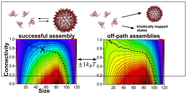
Grand canonical free energy landscapes (in kBT units) in the DC − s plane at the onset of the assembly reaction (t = 0) for a total capsid protein concentration of 20 μM and different dimer-dimer association free energies, ΔFn. At t = 0 the oversaturation state of the system was represented by the grand canonical ensemble free energy (Eq. 3). When ΔFn was −6.5 kBT (weak interaction), no assembly products were observed (a); At −7.5 kBT (moderate interaction), the assembly products at all the temperatures agreed with the thermodynamic model (blue symbols in Figure 5) (b); and at −8.5 kBT (strong interaction), deviations from the thermodynamic model were observed (red symbols in Figure 5) (c). Red arrows represent the directions along the minimum energy path from dimers to full capsid. Black arrows represent paths for forming unstable intermediates at the onset of assembly reactions. Crosses indicate that a path is unlikely. Panel (d) shows the initial grand canonical free energy at several points along the black arrow at the three interactions strength values. Figures S23-S25 plot the same energy landscapes in the s − c plane. (e) The cartons at the bottom correspond to atomic models of intermediate structures along the red and black paths, marked by the dots in panel (c).
When the association free energy is slightly higher than ΔFmin (Figure 8b), the global minimum shifts to the complete capsid state. In this case, the lowest energy path that connects the local minimum at the dimeric state and the global minimum at the full capsid state crosses a wide and flat free energy barrier (between s = 20 and s = 85). As the contour lines are roughly parallel to the lowest energy path throughout the reaction most of the assembly path from dimer to capsid, the probability for going off-path (in other words, moving away from the lowest energy path and crossing multiple contour lines barriers as illustrated by the black arrow) is very low. This kind of free energy landscape maximizes successful assembly.
As the association free energy is further strengthen to ~ ΔFmax (Figure 8c) the contour lines deviate from the lowest energy path (for example the contour marked by the black arrow), which increases the probability of sampling unstable structures (low DC). Once mistakes are made, strong association energy creates high barriers for returning to the lowest energy path which may require simultaneous dissociation of several dimer subunits. Also, the concentration of free dimers may at this stage be too low for filling holes in the structure. Similar kinetically trapped structures may form at high protein concentrations (Figure S19b and c).
The apparent narrow range of inter-subunit association free energy that can lead to successful assembly without accumulation of kinetic traps is consistent with earlier predictions.4,10,44,45 Theoretical studies using either coarse grained molecular dynamics simulations to follow the formation of T = 3 capsids44 or a combination of simulations and theory to elucidate possible mechanisms in kinetically trapped viral and general self-assembly processes45,46 discussed the crucial role of weak and reversible interactions for avoiding kinetic traps. In a reversible process, mistakes may be corrected during the growth of the assembled cluster, keeping the assembly path close to its most stable state (for a given cluster size). At the same time, the subunit concentration slowly decays, allowing the system to attain equilibrium. Under those conditions, the reaction path may be described by considering a small number of intermediate structures at the lowest energy path, as predicted by our grand canonical free energy landscape (Figure 8).
Figure 9a shows the minimum grand canonical free energy path at the onset of the assembly reaction (red arrows in Figure 8), predicted by our model (choosing only cmax (s) in Equation 3), as a function of size, s, at different ΔF4 values. As ΔF4 becomes more negative the barrier for assembly decreases from 50 to 12 kBT and the critical assembly size, beyond which assembly continues downhill in the energy landscape, decreases from 43 to 13 dimers. Notably, our free energy landscapes predict that no local minima are expected beyond the assembly barrier. At high ΔF4, local minima exist at smaller intermediates, where the most dominant and stable intermediate is a complete face of a T = 4 capsid, comprising 10 dimers. These results show that at strong association free energy, both the thermodynamic barrier for assembly and the barriers for creating less stable intermediates are very small and therefore the assembly process is expected to be kinetically controlled and sensitive to solution conditions and initial protein concentration. Aggressive assembly conditions can lead to a crossover from successful assembly to kinetically trapped reactions.47 As the assembly barrier is relatively flat, we expect a fast depletion of dimers and increase in the concentrations of a broad range of off-pathway intermediates. The higher probability for accumulation of unstable intermediates and the low concentration of free dimer may lead to misassembled particles, as detected in our SAXS measurements.
Figure 9:

The initial grand canonical ensemble free energy as a function of the size, s, of growing T = 4 and T = 3 capsids intermediates, along the minimum free energy path, at initial protein concentration of 20 μM. The minimal free energy path was calculated at different dimer-dimer association free energies, ΔF4 and α parameter as indicated. The grey broken line indicates the free energy level of the soluble dimer. (a) Initial free energy curve of the growing T = 4 capsid at four different association free energies. The bottom left inset shows the change in the free energy barrier, Δmax in kBT units and the size, s*, of the intermediate at the peak of the barrier, at each ΔF4. In addition to the expected decrease in Δmax with increasing ΔF4, there are local free energy minima at intermediates that are smaller than s*. The deepest local minimum appears at an intermediate of ten dimers, corresponding to the formation of a complete icosahedron face. (b) and (c): Comparison between the free energy per dimer in a complex (b) and per particle (c), as a function of s, for T = 4 and T = 3 capsids for two assembly conditions. Panel (c) shows that the free energy barrier is approximately similar for both capsids. Following the barriers, however, the free energy slope is steeper for the T = 3 capsid.
Finally, Figures 9b and c compare the minimum grand canonical free energy paths at the onset of the assembly of T = 3 and T = 4 capsids when the association free energies are moderate (Figure 8b) or strong (Figure 8c). The free energy per dimer (Figure 9b) and the free energy per particle (Figure 9c) are similar as long as the intermediates are smaller than the size of the intermediates at the highest free energy barrier. Beyond the barrier, however, the slope of the T = 3 free energy landscape is steeper37 but eventually complete T = 4 is more stable than complete T = 3.
Materials and Methods
Samples preparation
The N-terminal truncated dimer, cp149, was expressed in E.coli using a pET 11-based vector and purified as described.50 Stored samples of cp149 dimer often had small concentrations of large complexes. To start the assembly reaction from pure capsid protein dimer, samples of cp149 were treated with urea to dissociate complex; the samples were desalted and could be kept for several days at 4 °C and low ionic strength. Prior to SAXS data collection, purified cp149 dimer was dialyzed for 1.5 h three times at 4 °C, once against 3M urea in 50 mM Tris-HCl buffer at pH 7.5, and then twice against 50 mM HEPES buffer at pH 7.5. Figure 2 shows the scattering from 25 μM cp149 that was measured after the third dialysis. Protein concentration was determined by uv-vis absorbance using an extinction coefficient of 60,900 M−1cm−1. Cp149 dimer and 5× salt solution (5× NaCl and 50mM HEPES buffer at pH 7.5) were mixed at volume fractions of 4:1, respectively. This ratio minimized protein dilution and allowed better signal-to-noise ratio in scattering measurements. The mixed solution was equilibrated at 4 °C, room temperature, or 36 °C for ~5 hours prior to SAXS data collection. The scattering from the pure dimer solution, shown in Figure 2, was measured at 9 °C immediately following dialysis. For the measurements presented in Figure S20, cp149 was treated with 2 mM Dithiothreitol (DTT) prior to the urea treatment and the final buffer exchange to 50 mM HEPES pH 7.5 was done using a PD-10 desalting column. For these measurements 56 μM of cp149 protein were either mixed with 5× NaCl solution or gradually dialyzed against NaCl solution to reach the final salt concentration. The gradual dialysis protocol included four dialysis steps to slowly increase the NaCl concentration to 1 M: 0 to 100 mM, 100 to 300 mM, 300 to 500 mM, and 500 to 1000 mM.
SAXS Measurement Setup and Data Reduction.
Solution small X-ray scattering (SAXS) measurements of capsid assembly, shown in Figures 2, 3 and S19, were performed at the P12 EMBL BioSAXS Beamline (headed by D. Svergun) in PETRA III (DESY, Hamburg).51 Measurements were taken using an automated sample changer setup52 in which samples were stored on a temperature controlled plate and injected into a 2 mm diameter quartz capillary that was previously equilibrated at a desired temperature. The wavelength of the incident X-ray beam was 0.124 nm and the scattering intensity was recorded on a single-photon 2D PILATUS 2M pixel detector (DECTRIS). The products of the NaCl induced assembly reactions were measured at temperatures of 9, 25 and 36 °C to prevent samples from re-equilibrating. The sample-to-detector distance was 3 m, resulting in qmin = 0.025 nm−1 and qmax = 4.8 nm−1. For each assembly condition, between 30 and 35 μL of sample were injected to the measurement cell and between 30 to 35 frames were measured while the sample was flowing through the capillary. The exposure time per frame was 50 ms. Measurements shown in Figure S20 were performed at ID02 beamline (headed by T. Narayanan) in ESRF (Grenoble). These measurements were taken using the flow-cell setup which included a temperature controlled, 2 mm thick, quartz capillary.53 The wavelength of the incident beam was 0.995 nm and the scattered intensity was recorded on a FReLoN 16M Kodak CCD detector. Measurements were taken at 25 °C at sample-to-detector distance of 2.5 m that resulted in a q-range of 0.03-2.7 nm−1. For each experiment, between 40 and 50 μL of sample was injected to the measurement cell and 30 frames were recorded with exposure times that lasted between 50 and 100 ms. Background measurements were taken before and after each sample. The background solutions contained the same solution as the sample apart from the protein and was measured under identical conditions. Frames of data were normalized to the intensity of the transmitted beam, and azimuthally averaged to yield the scattering intensity curve as a function of the magnitude of the scattering vector, q.54 Background scattering curves were averaged and the averaged background signal was subtracted from the averaged sample signal to give the final scattering intensity curve of the assembly reactions, as explained in our earlier papers.30,55,56 Measurements were repeated at SWING beamline (J. Perez) in Soleil synchrotron (Gif-sur-YVETTE). Detailed experimental description of this setups were provided elsewhere.57-60
Graph representation of capsids
is an icosahedral capsid intermediate, whose triangulation number is n, and is made of s dimer subunits, which are forming c dimer - dimer contacts. The capsid intermediate configurations were represented as a weighted undirected graph. Each vertex of the graph represented the geometric center of a dimeric subunit whereas each edge corresponded to an inter-dimer interaction. In our case, each dimer was in either T = 3 or T = 4 symmetry and could interact with four neighboring dimers. The degree of each vertex in our graphs was therefore four. As not all the inter-dimer interactions were equivalent, we weighted the edges according to the center-to-center distance between two interacting dimers that defined an edge. Within this representation, the complete capsids were considered as a weighted graphs of 4-degrees with 90 vertices and 180 edges, in the case of T = 3, and 120 nodes and 240 edges, in the case of T = 4. According to the crystal structure there were two types of dimer positions both for the T = 3 and the T = 4 symmetries that formed three types of inter-dimer interactions in the T = 4 symmetry and two types in the T = 3 symmetry. We defined the two positions as position A and position B and therefore the edges could be of type AA, AB, or BB. In the simulations, each intermediate structure was represented by an s × 4 matrix, where each row corresponded to a vertex and contained the indexes of its neighboring vertices. Based on the matrix, we mapped the occupied vertices and edges of each intermediate.
The weighted undirected full capsid graphs were then represented by GT=n = (V, E, ET), where V, E and ET are the sets of vertices (v1, …, ), edges (e1, …, en·60) and edge types (et1, …, etn·60), respectively, where the possible edge types were eti ∈ {AA, AB, BB}. intermediate structures were represented by subgraphs (see below). Figure 1 shows the reduction of the two capsid geometries to their graph representations.
Monte Carlo simulations
Using our graph representation of capsids, we performed MC simulations to obtain the canonical partition function, Zn, of capsid intermediates, in the size-contact phase space:
| (4) |
ΔFn,c is the association free energy of an intermediate complex with c contacts in a T = n symmetry. Ωn,s,c is the number of different possible ways to create intermediates of size s with c inter-subunit contacts in a T = n symmetry. The distribution of microstates that dictate the values of Ωn,s,c are computed explicitly from the simulation.
Simulation phase space
The simulations were based on the graph representations of T = 3 or T = 4 capsid intermediates. represented a subgraph of GT=n at the i-th iteration of the MC simulation. Vi, Ei, and ETi were subsets of V, E, and ET, respectively. The size, si (or number of occupied vertices), and connectivity, ci (or number of contacts between dimers), of the i-th iteration where calculate from the size of Vi and Ei subsets. As each vertex in the subgraph corresponded to a specific dimer, we could represent the structure of each intermediate as a binary occupancy vector of size n · , in which 1 corresponded to an occupied position and 0 to an unoccupied position.
Umbrella sampling method
Simple MC procedure could not properly sample the distribution of intermediate states of Hepatitis B capsids, because the number of states combinatorially increases with the number of subunits. In simulations with low dimer-dimer association energies, the fast increase in the number of states with intermediate size ,s, precluded sampling of energetically favorable states, because energetically favored states occupy a negligible part of the size (s) - contact (c) phase-space. Higher association energies generate high dissociation energy barriers that confined the simulation sampling to a small subspace and exclude kinetically favorable intermediates. To correctly explore the entire distribution of intermediate states, we performed MC simulations with zero association energy and used an umbrella sampling procedure.61 We separately scanned the s coordinate and the c coordinate, using two sets of umbrella potentials. For the size coordinate,
| (5) |
where and are the maximal and minimal intermediate sizes, respectively, at umbrella potential Ej. The width of the umbrella potential windows, given by , were between 5 and 7 for different j values along the s coordinate. For a given size, si, where si ∈ (1, …, n · ), we scanned the number of contacts, c, axis with another umbrella potential defined as,
| (6) |
where and are the minimum and maximum number of contacts, respectively, of intermediates of size si. The width of the umbrella potential windows were between 4 and 6 contacts. Within each umbrella potential, the two dimensional size-contact probability distribution was constructed. As the contact association free energy was set to zero, the probability distributions per umbrella potential, Ej, were defined as, for the size axis, and for the contact axis at a given size, si, where were the total recorded frames along the simulation at umbrella potential .
Allowed steps, acceptance criteria and detailed balance
The metropolis algorithm62 was used in our MC simulations, where the graph representation of capsid intermediates defined the discrete set of possible steps. As described, one simulation set scanned the s coordinate, from which the intermediate size distribution was obtained. The second simulation set scanned the c coordinate, within subgraphs with s occupied vortexes, from which the connectivity distributions at a given s value was obtained.
Simulation along the s axis.
The allowed steps in the simulations were either adding or removing a single vertex. The simulation followed the following procedure: Given the current state, , of the system, a list of all the possible positions for adding or removing a subunit were created based on the nearest neighbors of each vertex. The size of this list gave the total number of allowed steps, Ni. In addition, a list of all the articulation points (APs) of the subgraph (in other words, vertices that disconnect the subgraph) was generated using depth first search (DFS) algorithm.63
At a given state of the simulation, μs, a random vertex position, v, was chosen from the list of the Ni allowed positions. If v was an empty vertex, the simulation tried to add a new vertex to the current subgraph. If v was an occupied vertex, the simulation tried to remove the vertex from the subgraph. To maintain detailed balance, if v was an occupied articulation point, any attempt of the simulation to change the current state was denied, as we allowed only addition or removal of a single vertex at each iteration. Removal of an articulation point would lead to dissociation of multisubunit oligomers, which had to be denied because the reverse process was also not allowed. The new state was then given by νs′, where s′ is the number of occupied vertices of the new state.
To maintain the condition of detailed balance at equilibrium, the probability to proceed from the current state, μs, to the new state, νs′, had to satisfy64
| (7) |
where, C(νs′) is the probability to select the new state, νs′, and A(μs → νs′) is the probability to accept the step from state μs to νs′. Similar conversion was applied to the reverse process. As within each umbrella potential, Eνs′ = Eμs = 0 (Equation 5) we got:
| (8) |
If s′ > s, we defined A(νs′ → μs) ≡ 1, hence , and , and , where Nμs and Nνs′ are the total numbers of allowed steps at states μs and , respectively. We can summarize the acceptance criteria as follows:
| (9) |
Simulation along the c axis.
The simulations that sampled the connectivity distribution were performed under a fixed number of occupied vertices, s. At each iteration, the allowed steps changed the position of one vertex, using the following procedure. At a given state, , a vertex, v, was randomly selected from the set, Vi, of s occupied vertices. If v was an articulation point the step was denied, otherwise the vertex was removed and an intermediate state of size s − 1, defined as , was obtained. At intermediate state , the list of all the possible sites where a new vertex can be added was created, based on the nearest neighbors of the occupied vertices. A random position was then selected from the list, and its occupancy was changed from an empty to an occupied vertex.
Reduction to unique structures
The simulations described so far, over estimated the number of states because translated and rotated subgraphs were treated as distinct states, even though they were structurally identical. To include in our probability distributions only unique structures from each simulation, we introduced a three-step classification test to discard replicated states. The first classification was based on the graph representation of the state, namely the occupied vertices and the connectivity between them. The second classification was based on the pair distribution function of the center of mass of the subunits. The third classification, was based on complete alignment of the 3D structures.
Graph representation
Based on the graph representation of the structures, two structures could be considered identical only if they were isomorphic, namely they contained the same number and type of vertices and edges. Isomorphic graphs were tested using the built-in function of networkX package,65 which uses the VF2 algorithm.66
Pair distribution function.
The graph representation did not contain the entire structural information. In some cases, two different states could have isomorphic graphs (Figure S11). To determine whether two structures were identical or not, we compared the pair distribution function of the geometrical centers of the subunits. As each vertex in the graph was linked to a specific coordinate in 3D space, the occupancy vector could be used to generate a histogram of the distances between all the subunit pairs in the complex. The pair distribution functions were binned into a vector of integers, , where the value at each index, hi, represented the occurrence of distances within the limits of the i–th bin. Using bin sizes ranging between 0.1 Å and 4nm, we could build a unique signature for each state, namely, two structures with the same signature had exactly the same pair distribution functions.
Complete alignment between two structures
In special cases (chiral structures, for example), the pair distribution function and the graph representation criteria could still under estimate the number of states (Figure S12 and Section 2c). We therefore introduced an alignment test, which exploited the entire 3D structural information. When two structures had isomorphic graph representations, G1 and G2, and identical signatures, we checked whether the structures could be fully aligned.
Let M be the set of possible mapping options between G1 and G2. For each m ∈ M, we created two s×3 matrices, A1 and A2, containing the x, y, z coordinates of the geometric centers of all the subunits in the complexes (where the origin was at the geometric center of the entire complex). We defined the covariance matrix, , and found its singular value decomposition (SVD), C12 = UΣV⊺, where, U and V were unitary matrices and Σ was a diagonal matrix with non-negative real values along its diagonal. The rotation matrix, R, which minimized the squared norm of the residual matrix, ∥D12∥2, was then give by67
where D12 ≡ RA2 − A1. Two structures were considered identical if the minimum norm of their residual matrix, ∥D12∥, was 1 Å or less. The loop over m ∈ M was terminated, when the algorithm identified a mapping, m, which satisfied the minimization criterion.
Practically, the probability of sampling two different structures with identical pair distribution functions was extremely low for large s. We found that the number of states, based on the pair distribution signature alone, was similar to the number of states obtained by the three-step procedure, whereas the pair distributions were significantly simpler to compute. Hence, when the number of subunits in the complexes was between 30 and n · − 5, the alignment test was not applied. For s > n · − 5, we performed the three-step analysis on the "inverse" graphs, which we defined as the graph that contained the unoccupied vertices of each iteration, , and the edges connecting them, with ∈ V − Vi.
Unifying the probability distribution
Once the distribution of states within each umbrella potential was obtained, the distributions were unified into a single s − c distribution. By selecting the overlap between two adjacent potentials to satisfy or , the relative scale between subsequent potentials, rj,j+1, was given by
for the s axis. A similar expression was applied for the c axis. The absolute scale Ak of umbrella potential k was therefore , where k ≥ 2. Once the scaling for all the potentials was set, the combined distribution was renormalized so that Σs Σc P(s, c) = 1.
SAXS curves calculations
To generate a pool of scattering models we randomly selected between 1 and 5 different structures for each intermediate (representing a point in the s − c plane). Each structure was defined by a list of s parameter vectors, each contained the position (x, y, z coordinates) of the geometric center of a dimer and the three Euler angles (α, β, γ) that defined its orientation. The dimer subunit was taken from the protein data bank (PDB ID 2G33)48 and was docked into both T = 3 and T = 4 symmetries. The parameters for calculating the scattering intensity of the entire set were chosen by fitting the expected scattering intensity from the atomic structure of the dimer to the experimental scattering data from a pure solution of 25 μM cp149 in 50 mM HEPES buffer pH 7.5, at room temperature (Figure 2). The fitting procedure was done using our home developed software, D+ (https://scholars.huji.ac.il/uriraviv/software/d-software).30,31 The electron density of the solvent was set to the electron density of water (333 ), and the thickness and electron density of the solvation layer around the protein were our fitting parameters. Once the best fitted parameters were found, the scattering amplitude of the dimer was saved and used for calculating the scattering intensity, (q), of all the other intermediates in the pool, according to
where, is the scattering amplitude of the j-th dimer whose orientations in the complex is given by the of rotation matrices Aj. is the geometric center position of the j-th dimer, and ⟨…⟩Ωq represents the orientation averaging of the scattering intensity. All models were then scaled to the absolute scale (see derivation in Section 1a in SI) according to
The scaling corresponds to a protein concentration of 1 (C = 1) with where is the molecular weight of the dimer subunit including its solvation layer. ID+ (q) is the scattering intensity computed by D+ software, in which the Thomson scattering length is set to unity.
Scattering amplitude of the atomic model of the dimer in solution
The scattering amplitude of the j-th atom in vacuo (using the five Gaussian approximation) is:
| (10) |
The coefficients ak, bk, and c are the Cromer-Mann coefficients, given in units of the Thomson scattering length, r0. Note that in our analysis software, D+, r0 is set to 1.30,31 To account for the solvent excluded volume of the atoms, we subtracted a Gaussian sphere from each atom, where the center of the sphere was located at the atom coordinate.68-70 Our analysis software, D+,31 subtracts the Fourier transform of the following normalized Gaussian sphere:
where is the volume of atom j, and Vm = Σj Vj is the mean atomic volume over the entire molecule. rj is an effective atomic radius (dictated by the type of atom) and ρ0 is the mean solvent electron density. The scattering amplitude from atom j after subtracting the contribution of the solvent is:
| (11) |
The solvent contribution can be modulated like
where
is used to uniformly adjust Vm and c1 is a scaling factor.71
The solution scattering amplitude from a dimer, given by a list of its n atoms, whose coordinates are , was:
Solvation Layer
The solvent excluded volume was calculated by discretizing space into 0.125 A3 voxels. Each voxel was marked as occupied if at least one atom’s coordinate was within that atom’s radius. A probe with a radius of 1.4 A, which corresponds to the radius of a water molecule, determined the accessible surface of the protein. All voxels that were within the solvation thickness, ΔSolvent Layer, of the protein surface and were not occupied by an atom were marked as occupied by a solvation layer, and assumed a mean electron density, ρSolvent Layer. The contribution of the solvation layer to the scattering amplitude was computed as the sum over the scattering amplitudes from the collection of voxels comprising the solvation layer. The scattering amplitude of the jth voxel of dimensions, ωj, τj, and μj, whose center was at was:72
| (12) |
The amplitude of the solvation layer was then:
| (13) |
The scattering amplitude of a solvated molecule was:
| (14) |
where () is the scattering amplitude from the molecule in solution (without the solvation layer contribution).
Resolution correction of the models
To account for the finite resolution of the measurement, we included a resolution correction to our calculated models set.73 The corrected intensity, Icorr, as a function of q for each computed model intensity, Imodel, was:
where σq was calculated according to the geometry of our setup to be 0.01 nm−1.74
Sensitivity analysis of SAXS models using a clustering algorithm
To estimate the sensitivity of our fitting results relative to the signal to noise ratio (SNR) we applied clustering algorithm on the expected scattering intensities in the size and contact plane. Clustering of the SAXS models, as presented in Section 1d in the SI and in Figure S7, was done on the set of models that was used to analyze our SAXS data. The number of clusters rapidly increased as the size of the intermediates decreased (as the size of the particle decreases the effect on the scattering curve of adding or moving subunits is larger). Hence, we applied the clustering procedure to models whose s values were within the top 33% of each capsid symmetry. The clustering was done on the weighted matrix, MT=4 and MT=3 given by,
and,
where each column in the matrix corresponds to the computed scattering intensity, (q), of the atomic model of intermediate with smin = 80 or 60 for T = 4 and T = 3, respectively. The models were computed between q1 = 0.1 nm−1 and qN = 1.5 nm−1, neglecting the high q range where the SNR was low. The intensities were weighted according to the measured noise level, σ (qi). The dimensions of the matrices were N × mT=4 and N × mT=3 where the total number of q values that were considered was N = 280, and the number of intermediate structures were mT=4 = 1361 and mT=3 = 749, for the T = 4 and T = 3 symmetries, respectively.
To reduce the dimensions of the matrices, prior to the clustering algorithm, SVD analysis was applied. The analysis revealed the ranks, r and r′ of the MT=4 and MT=3 matrices, respectively. Hence, the dimensions of the matrices decreased to r × mT=4 and r′ × mT=3, where r = 23 and r′ = 15. The ranks were determined by demanding that the maximum deviation between the SVD-reconstructed matrix and the original matrix will be 0.01σ or less. We than applied the k-means algorithm75 onto the reduced space, in order to classify the m models onto the minimal number of clusters, k. The minimal k was found by demanding that all the models that were classified into the same cluster will fulfill the following χ2 condition,
where (qi) is a model that was classified into the jth cluster, and (qj) is the modeled scattering intensity of the centroid of the jth cluster. Using this method, we classified the MT=4 and MT=3 matrices into 221 and 107 clusters, respectively.
Thermodynamic model
Consider the following set of coupled assembly reactions, induced by increasing the salt concentration:
s is the number of dimer molecules, D, which assemble into a icosahedral capsid intermediate, whose triangulation, T, number is n, and c is the number of its dimer - dimer contacts. n is either 3 or 4 and νn,s,c and νD are the stoichiometric coefficients of and D, respectively (note that νD = ν3,1,0 = ν4,1,0). From mass conservation we get:
Our aim is to determine the distribution of intermediates at equilibrium.
The degeneracy, Ωn,s,c, of each intermediate state in the s − c phase space was obtained from our MC simulations (in the simulations, s was the number of occupied vertices and c was the number of edges). At temperature T, the equilibrium probability distribution of intermediate structures in the canonical ensemble was calculated as a function of the dimer-dimer association free energy per contact, ΔFn, by adding Boltzmann factor to the number of possible unique intermediate states (the degeneracy factor), Ωn,s,c, obtained from our zero association free energy simulations:
Z is the partition function in the canonical ensemble:
where kB is Boltzmann’s constant. To obtain the distribution in the grand canonical ensemble, the translational entropy of the intermediate structures was taken into account. Following earlier theoretical models,76-79 we assumed an implicit solvent background (rather than explicitly consider the contribution of the water molecules or salt ions to the free energy).
The dimer molecules could be in each of the intermediate states. The occupancy of each state was described on the mole fraction scale, where Xn,s,c, is the molar fraction of dimer subunits, incorporated into intermediate, and is given by . nn,s,c is the number of intermediate of type and ntotal is the total number of molecules. ntotal = ndimer + nwater, where ndimer is the total number of dimer molecules in all the intermediates and nwater is the total number of water molecules. As the dimer is much larger than a water molecule, the total number of molecules is a function of the total dimer concentration. Therefore the general definition of Xn,s,c using intensive quantities (molar concentrations, c, rather than number of molecules) is , where Nw is the number of excluded water molecules per dimer. The dimer excluded volume was calculated in D+31 based on the dimer atomic model, using voxel size of 0.05 nm and a probe radius of 0.14 nm. The calculated volume was 28.5 nm3, corresponding to ~ 103 water molecules. The total dimer concentrations in our assembly reactions were between 20 and 40 μM, contributing a correction of ~ 10−2 M to the total concentration of molecules. We therefore neglected this correction and set ctotal ≃ cwater and , for the analysis at all our protein concentrations.76,77,79
From the conservation of mass we get,
| (15) |
where XTotal is the total molar fraction of dimer molecules. The range of s is a function of n, and the range of c is a function of both s and n.
The total Helmholtz free energy in the grand canonical ensemble is given by:
| (16) |
where Ntot is the total number of molecules (water and capsid protein dimer). ΔFn,s,c is the Helmholtz free energy gain for the formation of intermediates, approximated by:
| (17) |
The first term in Equation 17 is the formation free energy, in the molar fraction scale, of c dimer-dimer (independent) contacts and the second term in Equation 17 is the configurational entropy term, associated with the number of ways to form intermediates, given by Ωn,s,c. The second and third terms in Equation 16 come form the mixing entropy of all the intermediates (second term) and the contribution of the solvent to the mixing entropy (third term). The equilibrium distribution of intermediates is obtained by minimizing the total Helmholtz free energy subject to the constraint of Equation 15. Using the Lagrange multipliers method, the solution to the minimization problem is obtained by solving the following equation
where λ is the Lagrange multiplier. The result of the derivation is
| (18) |
hence, the distribution that minimizes the Helmholtz free energy is
| (19) |
To find the physical meaning of λ, we proceed as follows. The chemical potential of s dimers in intermediates is,
| (20) |
From Equations 18 and 20 we get that at equilibrium, the chemical potential per dimer at each of the intermediates is the same:
| (21) |
In particular, the chemical potential of a dimer in each of the intermediates must be equal to the chemical potential of the free dimer
| (22) |
By combining Equations 20 and 22, we find that the molar fraction distribution takes the following form:
| (23) |
By setting s = 1 in Equation 18 (or by comparing Equation 23 with Equation 19), we find that μ1 = λ. In other words, the Lagrange multiplier, λ, is the chemical potential of the free dimer in the solution, given by μ1 = kBT ln X1. By substituting μ1 to Equation 23 we get:
| (24) |
Equation 24, satisfies the law of mass action in the s − c phase-space.
Fitting the law of mass action
The parameters of our model were the total molar fraction of the protein, XTotal, which we know from the experiments, and the dimer-dimer association free energies, ΔFn, in the T = 3 and T = 4 symmetries. The total molar fraction was given by when Cprotein is the molar protein concentration in mol/L. The fitting parameters were ΔF4 and α, where ΔF3 = α · ΔF4. Since X1 is a function of ΔF4 and α to compute equation 24, we set the values of α and ΔF4 and numerically solved equation 15 by finding the value of X1, to minimize:
| (25) |
The resulting Xn,s,c molar fractions were then used to compute the expected solution X-ray scattering curve:
| (26) |
where In,s,c (q) was the scattering curve of the most probable intermediate and was the probability of finding that intermediate. Imodel (q) was then compared with the experimental scattering curve, Iexp (q). ΔF4 and α were then modified and the process repeated until the best fit to the experimental data was attained. The best fit criterion was minimal χ2 value, where
| (27) |
Iexp (qi) is the measured scattering intensity at qi, where qi is the magnitude of the momentum transfer vector. σi is the standard deviation of Iexp (qi), a is a total scaling factor and b is a constant value to correct the high q region for small inaccuracies (mainly owing to dark current contribution) when subtracting background scattering curves.
Conclusions
Our high resolution solution X-ray scattering data, MC simulations, and thermodynamic analysis reveal the distribution of capsid assembly reaction products over a wide range of conditions. The results extend earlier studies showing that dimer-dimer association free energy is a function of temperature and ionic strength by rigorously fitting high resolution data to a grand canonical free energy landscape. To construct this model we used umbrella sampling MC simulations of assembly leading us to estimate about 1030 possible intermediates. By applying Boltzmann weighting to this immense library we observed (i) a narrow swath of stable species that demarcated a series of en route reactions from dimer to capsid and (ii) that subtle changes in association energy could favor reaction pathways that led to kinetic traps with high barriers to return to an on-path route. For example, at strong dimer-dimer association free energy, high temperature, and high dimer concentration, kinetically trapped T=3-like nanoparticles, with a diameter of 28 nm, formed. These structures did not form when the salt concentration was slowly increased by dialysis, suggesting that these nanoparticles may not be stable T = 3 capsids. Similar flaws could also be achieved at high concentrations of cp149 because the grand canonical free energy landscape of the assembly reaction is also determined by reactant concentration. Successful assembly reactions are best realized within a narrow range of protein concentration and dimer-dimer association free energy. Thus, molecules that strengthen subunit-subunit interactions will be predicted to have antiviral effects.6,48,49 The approach established in the present work, can be applied to characterize other complex macromolecular assemblies. The mechanistic insight gained by our analysis provide means to describe bottom-up complex assembly reactions.
Supplementary Material
Acknowledgement
We thank Daniel Harries and Michael Hagan for very helpful discussions. We acknowledge Desy synchrotron at Hamburg, beamline P12 (D. Svergun and his team), the European Synchrotron Radiation Facility (ESRF) beamline ID02 (T. Narayanan and his team), and Soleil synchrotron, Swing beamline (J. Perez and his team), for provision of synchrotron radiation facilities and for assistance in using the beamlines. This project was supported by the NIH (award number 1R01AI118933). R.A. acknowledges support from the Kaye-Einstein Fellowship Foundation. U.R. and R.A. acknowledge financial support from the Israel Science Foundation (grant 656/17).
References
- (1).Katen S; Zlotnick A The thermodynamics of virus capsid assembly. Methods Enzymol. 2009, 455, 395–417. [DOI] [PMC free article] [PubMed] [Google Scholar]
- (2).Zlotnick A Are weak protein–protein interactions the general rule in capsid assembly? Virology 2003, 315, 269–274. [DOI] [PubMed] [Google Scholar]
- (3).Zlotnick A; Johnson JM; Wingfield PW; Stahl SJ; Endres D A theoretical model successfully identifies features of hepatitis B virus capsid assembly. Biochemistry 1999, 38, 14644–14652. [DOI] [PubMed] [Google Scholar]
- (4).Moisant P; Neeman H; Zlotnick A Exploring the paths of (virus) assembly. Biophys. J 2010, 99, 1350–1357. [DOI] [PMC free article] [PubMed] [Google Scholar]
- (5).Asor R; Khaykelson D; Ben-nun Shaul O; Oppenheim A; Raviv U Effect of Calcium Ions and Disulfide Bonds on Swelling of Virus Particles. ACS Omega 2019, 4, 58–64. [DOI] [PMC free article] [PubMed] [Google Scholar]
- (6).Zlotnick A; Mukhopadhyay S Virus assembly, allostery and antivirals. Trends Microbiol. 2011, 19, 14–23. [DOI] [PMC free article] [PubMed] [Google Scholar]
- (7).Uetrecht C; Barbu IM; Shoemaker GK; Van Duijn E; Heck AJ Interrogating viral capsid assembly with ion mobility–mass spectrometry. Nat. Chem 2011, 3, 126. [DOI] [PubMed] [Google Scholar]
- (8).Lutomski CA; Lyktey NA; Zhao Z; Pierson EE; Zlotnick A; Jarrold MF Hepatitis B Virus Capsid Completion Occurs through Error Correction. J. Am. Chem. Soc 2017, 139, 16932–16938, PMID: 29125756. [DOI] [PMC free article] [PubMed] [Google Scholar]
- (9).Hagan MF; Elrad OM Understanding the concentration dependence of viral capsid assembly kinetics - the origin of the lag time and identifying the critical nucleus size. Biophys. J 2010, 98, 1065–1074. [DOI] [PMC free article] [PubMed] [Google Scholar]
- (10).Endres D; Miyahara M; Moisant P; Zlotnick A A reaction landscape identifies the intermediates critical for self-assembly of virus capsids and other polyhedral structures. Protein Sci. 2005, 14, 1518–1525. [DOI] [PMC free article] [PubMed] [Google Scholar]
- (11).Morozov AY; Bruinsma RF; Rudnick J Assembly of viruses and the pseudo-law of mass action. J. Chem. Phys 2009, 131, 10B607. [DOI] [PubMed] [Google Scholar]
- (12).Garmann RF; Comas-Garcia M; Knobler CM; Gelbart WM Physical principles in the self-assembly of a simple spherical virus. Acc. Chem. Res 2015, 49, 48–55. [DOI] [PubMed] [Google Scholar]
- (13).Tresset G; Chen J; Chevreuil M; Nhiri N; Jacquet E; Lansac Y Two-dimensional phase transition of viral capsid gives insights into subunit interactions. Phys. Rev. Appl 2017, 7, 014005. [Google Scholar]
- (14).Kler S; Asor R; Li C; Ginsburg A; Harries D; Oppenheim A; Zlotnick A; Raviv U RNA encapsidation by SV40-derived nanoparticles follows a rapid two-state mechanism. J. Am. Chem. Soc 2012, 134, 8823–8830. [DOI] [PMC free article] [PubMed] [Google Scholar]
- (15).Li C; Kneller AR; Jacobson SC; Zlotnick A Single particle observation of SV40 vp1 polyanion-induced assembly shows that substrate size and structure modulate capsid geometry. ACS Chem. Biol 2017, 12, 1327–1334. [DOI] [PMC free article] [PubMed] [Google Scholar]
- (16).Kler S; Wang JC-Y; Dhason M; Oppenheim A; Zlotnick A Scaffold properties are a key determinant of the size and shape of self-assembled virus-derived particles. ACS Chem. Biol 2013, 8, 2753–2761. [DOI] [PMC free article] [PubMed] [Google Scholar]
- (17).Hu Y; Zandi R; Anavitarte A; Knobler CM; Gelbart WM Packaging of a polymer by a viral capsid: the interplay between polymer length and capsid size. Biophys. J 2008, 94, 1428–1436. [DOI] [PMC free article] [PubMed] [Google Scholar]
- (18).Auyeung E; Li TI; Senesi AJ; Schmucker AL; Pals BC; de La Cruz MO; Mirkin CA DNA-mediated nanoparticle crystallization into Wulff polyhedra. Nature 2014, 505, 73–77. [DOI] [PubMed] [Google Scholar]
- (19).Schwarz B; Uchida M; Douglas T Chapter One-Biomedical and Catalytic Opportunities of Virus-Like Particles in Nanotechnology. Adv. Virus Res 2017, 97, 1–60. [DOI] [PMC free article] [PubMed] [Google Scholar]
- (20).Pokorski JK; Steinmetz NF The art of engineering viral nanoparticles. Mol. Pharm 2011, 8, 29. [DOI] [PMC free article] [PubMed] [Google Scholar]
- (21).Loo L; Guenther RH; Basnayake VR; Lommel SA; Franzen S Controlled encapsidation of gold nanoparticles by a viral protein shell. J. Am. Chem. Soc 2006, 128, 4502–4503. [DOI] [PubMed] [Google Scholar]
- (22).Chen C; Daniel M-C; Quinkert ZT; De M; Stein B; Bowman VD; Chipman PR; Rotello VM; Kao CC; Dragnea B Nanoparticle-templated assembly of viral protein cages. Nano Lett. 2006, 6, 611–615. [DOI] [PubMed] [Google Scholar]
- (23).Douglas T; Young M Viruses: making friends with old foes. Science 2006, 312, 873–875. [DOI] [PubMed] [Google Scholar]
- (24).Uchida M; Klem MT; Allen M; Suci P; Flenniken M; Gillitzer E; Varpness Z; Liepold LO; Young M; Douglas T Biological containers: protein cages as multifunctional nanoplatforms. Adv. Mater 2007, 19, 1025–1042. [Google Scholar]
- (25).Jordan PC; Patterson DP; Saboda KN; Edwards EJ; Miettinen HM; Basu G; Thielges MC; Douglas T Self-assembling biomolecular catalysts for hydrogen production. Nat. Chem 2015, [DOI] [PubMed] [Google Scholar]
- (26).Ceres P; Zlotnick A Weak protein- protein interactions are sufficient to drive assembly of hepatitis B virus capsids. Biochemistry 2002, 41, 11525–11531. [DOI] [PubMed] [Google Scholar]
- (27).Stannard LM; Hodgkiss M Morphological irregularities in Dane particle cores. J. Gen. Virol 1979, 45, 509–514. [DOI] [PubMed] [Google Scholar]
- (28).Zhou J; Kondylis P; Haywood DG; Harms ZD; Lee LS; Zlotnick A; Jacobson SC Characterization of Virus Capsids and Their Assembly Intermediates by Multicycle Resistive-Pulse Sensing with Four Pores in Series. Anal. Chem 2018, 90, 7267–7274. [DOI] [PMC free article] [PubMed] [Google Scholar]
- (29).Lutomski CA; Lyktey NA; Pierson EE; Zhao Z; Zlotnick A; Jarrold MF Multiple Pathways in Capsid Assembly. J. Am. Chem. Soc 2018, 140, 5784–5790. [DOI] [PMC free article] [PubMed] [Google Scholar]
- (30).Ginsburg A; Ben-Nun T; Asor R; Shemesh A; Ringel I; Raviv U Reciprocal Grids: A Hierarchical Algorithm for Computing Solution X-ray Scattering Curves from Supramolecular Complexes at High Resolution. J. Chem. Inf. Model 2016, 56, PMID: 27410762. [DOI] [PubMed] [Google Scholar]
- (31).Ginsburg A; Ben-Nun T; Asor R; Shemesh A; Fink L; Tekoah R; Levartovsky Y; Khaykelson D; Dharan R; Fellig A; Raviv U D+: Software for High-Resolution Hierarchical Modeling of Solution X-Ray Scattering from Complex Structures. J. Appl. Crystallogr 2019, 52. [DOI] [PMC free article] [PubMed] [Google Scholar]
- (32).Jaynes ET Information theory and statistical mechanics. Phys. Rev 1957, 106, 620. [Google Scholar]
- (33).Levine RD An information theoretical approach to inversion problems. J. Phys. A Math. Gen 1980, 13, 91. [Google Scholar]
- (34).Levinthal C How to fold graciously. Mossbauer spectroscopy in biological systems 1969, 67, 22–24. [Google Scholar]
- (35).Packianathan C; Katen SP; Dann CE; Zlotnick A Conformational changes in the hepatitis B virus core protein are consistent with a role for allostery in virus assembly. J. Virol 2010, 84, 1607–1615. [DOI] [PMC free article] [PubMed] [Google Scholar]
- (36).Chen VB; Arendall WB III; Headd JJ; Keedy DA; Immormino RM; Kapral GJ; Murray LW; Richardson JS; Richardson DC MolProbity: all-atom structure validation for macromolecular crystallography. Acta Crystallogr. D 2010, 66, 12–21. [DOI] [PMC free article] [PubMed] [Google Scholar]
- (37).Harms ZD; Selzer L; Zlotnick A; Jacobson SC Monitoring assembly of virus capsids with nanofluidic devices. ACS Nano 2015, 9, 9087–9096. [DOI] [PMC free article] [PubMed] [Google Scholar]
- (38).Sun X; Li D; Wang Z; Liu Q; Wei Y; Liu T A dimorphism shift of hepatitis B virus capsids in response to ionic conditions. Nanoscale 2018, 10, 16984–16989. [DOI] [PubMed] [Google Scholar]
- (39).Kegel WK; van der Schoot P Competing hydrophobic and screened-Coulomb interactions in hepatitis B virus capsid assembly. Biophys. J 2004, 86, 3905–3913. [DOI] [PMC free article] [PubMed] [Google Scholar]
- (40).Pierson EE; Keifer DZ; Selzer L; Lee LS; Contino NC; Wang JC-Y; Zlotnick A; Jarrold MF Detection of late intermediates in virus capsid assembly by charge detection mass spectrometry. J. Am. Chem. Soc 2014, 136, 3536–3541. [DOI] [PMC free article] [PubMed] [Google Scholar]
- (41).Luque A; Reguera D; Morozov A; Rudnick J; Bruinsma R Physics of shell assembly: Line tension, hole implosion, and closure catastrophe. J. Chem. Phys 2012, 136, 184507. [DOI] [PubMed] [Google Scholar]
- (42).Singh S; Zlotnick A Observed hysteresis of virus capsid disassembly is implicit in kinetic models of assembly. J. Biol. Chem 2003, 278, 18249–18255. [DOI] [PubMed] [Google Scholar]
- (43).Hagan MF Modeling viral capsid assembly. Adv. Chem. Phys 2014, 155, 1. [DOI] [PMC free article] [PubMed] [Google Scholar]
- (44).Rapaport D Molecular dynamics study of T= 3 capsid assembly. J. Biol. Phys 2018, 44, 147–162. [DOI] [PMC free article] [PubMed] [Google Scholar]
- (45).Hagan MF; Elrad OM; Jack RL Mechanisms of kinetic trapping in self-assembly and phase transformation. J. Chem. Phys 2011, 135, 104115. [DOI] [PMC free article] [PubMed] [Google Scholar]
- (46).Lazaro GR; Hagan MF Allosteric control of icosahedral capsid assembly. J. Phys. Chem. B 2016, 120, 6306–6318. [DOI] [PMC free article] [PubMed] [Google Scholar]
- (47).Michaels TC; Bellaiche MM; Hagan MF; Knowles TP Kinetic constraints on self-assembly into closed supramolecular structures. Sci. Rep 2017, 7, 12295. [DOI] [PMC free article] [PubMed] [Google Scholar]
- (48).Bourne CR; Finn M; Zlotnick A Global structural changes in hepatitis B virus capsids induced by the assembly effector HAP1. J. Virol 2006, 80, 11055–11061. [DOI] [PMC free article] [PubMed] [Google Scholar]
- (49).Venkatakrishnan B; Zlotnick A The structural biology of hepatitis B virus: form and function. Annu. Rev. Virol 2016, 3, 429–451. [DOI] [PMC free article] [PubMed] [Google Scholar]
- (50).Zlotnick A; Ceres P; Singh S; Johnson JM A small molecule inhibits and misdirects assembly of hepatitis B virus capsids. J. Virol 2002, 76, 4848–4854. [DOI] [PMC free article] [PubMed] [Google Scholar]
- (51).Blanchet CE; Spilotros A; Schwemmer F; Graewert MA; Kikhney A; Jeffries CM; Franke D; Mark D; Zengerle R; Cipriani F; Fiedler S; Roessle M; Svergun DI Versatile sample environments and automation for biological solution X-ray scattering experiments at the P12 beamline (PETRA III, DESY). J. Appl. Crystallogr 2015, 48, 431–443. [DOI] [PMC free article] [PubMed] [Google Scholar]
- (52).Round A; Felisaz F; Fodinger L; Gobbo A; Huet J; Villard C; Blanchet CE; Pernot P; McSweeney S; Roessle M; Svergun DI; Cipriani F BioSAXS Sample Changer: a robotic sample changer for rapid and reliable high-throughput X-ray solution scattering experiments. Acta Crystallogr. D 2015, 71, 67–75. [DOI] [PMC free article] [PubMed] [Google Scholar]
- (53).Van Vaerenbergh P; Léonardon J; Sztucki M; Boesecke P; Gorini J; Claustre L; Sever F; Morse J; Narayanan T An upgrade beamline for combined wide, small and ultra small-angle x-ray scattering at the ESRF. Proceedings of the 12th International Conference on Synchrotron Radiation Instrumentation (SRI2015). 2016; p 030034. [Google Scholar]
- (54).Hammersley A FIT2D: a multi-purpose data reduction, analysis and visualization program. J. Appl. Crystallogr 2016, 49. [Google Scholar]
- (55).Asor R; Ben-nun Shaul O; Oppenheim A; Raviv U Crystallization, Reentrant Melting, and Resolubilization of Virus Nanoparticles. ACS Nano 2017, 11, 9814–9824. [DOI] [PMC free article] [PubMed] [Google Scholar]
- (56).Ginsburg A; Shemesh A; Millgram A; Dharan R; Levi-Kalisman Y; Ringel I; Raviv U Structure of Dynamic, Taxol-Stabilized, and GMPPCP-Stabilized Microtubule. J. Phys. Chem. B 2017, 121, 8427–8436. [DOI] [PubMed] [Google Scholar]
- (57).David G; Pérez J Combined sampler robot and high-performance liquid chromatography: a fully automated system for biological small-angle X-ray scattering experiments at the Synchrotron SOLEIL SWING beamline. J. Appl. Crystallogr 2009, 42, 892–900. [Google Scholar]
- (58).Nadler M; Steiner A; Dvir T; Szekely O; Szekely P; Ginsburg A; Asor R; Resh R; Tamburu C; Peres M; Raviv U Following the structural changes during zinc-induced crystallization of charged membranes using time-resolved solution X-ray scattering. Soft Matter 2011, 7, 1512–1523. [Google Scholar]
- (59).Louzon D; Ginsburg A; Schwenger W; Dvir T; Dogic Z; Raviv U Structure and Intermolecular Interactions between L-Type Straight Flagellar Filaments. Biophys. J 2017, 112, 2184–2195. [DOI] [PMC free article] [PubMed] [Google Scholar]
- (60).Fink L; Feitelson J; Noff R; Dvir T; Tamburu C; Raviv U Osmotic stress induced desorption of calcium ions from dipolar lipid membranes. Langmuir 2017, [DOI] [PubMed] [Google Scholar]
- (61).Chandler D Introduction to modern statistical mechanics; Oxford University Press, 1987. [Google Scholar]
- (62).Metropolis N; Rosenbluth AW; Rosenbluth MN; Teller AH; Teller E Equation of state calculations by fast computing machines. J. Chem. Phys 1953, 21, 1087–1092. [Google Scholar]
- (63).Tarjan R Depth-First Search and Linear Graph Algorithms. SIAM J. Comput 1972, 1, 146–160. [Google Scholar]
- (64).Newman M; Barkema G Monte Carlo Methods in Statistical Physics chapter 1–4; Oxford University Press: New York, USA, 1999. [Google Scholar]
- (65).Hagberg AA; Schult DA; Swart PJ Exploring Network Structure, Dynamics, and Function using NetworkX. Proceedings of the 7th Python in Science Conference. Pasadena, CA USA, 2008; pp 11 – 15. [Google Scholar]
- (66).Cordella LP; Foggia P; Sansone C; Vento M An improved algorithm for matching large graphs. 3rd IAPR-TC15 workshop on graph-based representations in pattern recognition. 2001; pp 149–159. [Google Scholar]
- (67).Eggert DW; Lorusso A; Fisher RB Estimating 3-D rigid body transformations: a comparison of four major algorithms. MACH. VISION APPL 1997, 9, 272–290. [Google Scholar]
- (68).Fraser R; MacRae T; Suzuki E An improved method for calculating the contribution of solvent to the X-ray diffraction pattern of biological molecules. J. Appl. Crystallogr 1978, 11, 693–694. [Google Scholar]
- (69).Svergun D; Barberato C; Koch MH CRYSOL – a program to evaluate X-ray solution scattering of biological macromolecules from atomic coordinates. J. Appl. Crystallogr 1995, 28, 768–773. [Google Scholar]
- (70).Grudinin S; Garkavenko M; Kazennov A Pepsi-SAXS: an adaptive method for rapid and accurate computation of small-angle X-ray scattering profiles. Acta Crystallogr. D 2017, 73. [DOI] [PubMed] [Google Scholar]
- (71).Schneidman-Duhovny D; Hammel M; Tainer JA; Sali A Accurate SAXS profile computation and its assessment by contrast variation experiments. Biophys. J 2013, 105, 962–974. [DOI] [PMC free article] [PubMed] [Google Scholar]
- (72).Székely P; Ginsburg A; Ben-Nun T; Raviv U Solution x-ray scattering form factors of supramolecular self-assembled structures. Langmuir 2010, 26, 13110–13129. [DOI] [PubMed] [Google Scholar]
- (73).Ben-Nun T; Ginsburg A; Székely P; Raviv U X+: a comprehensive computationally accelerated structure analysis tool for solution x-ray scattering from supramolecular self-assemblies. J. Appl. Crystallogr 2010, 43, 1522–1531. [Google Scholar]
- (74).Pauw BR Everything SAXS: small-angle scattering pattern collection and correction. J. Phys. Condens. Matter 2013, 25, 383201. [DOI] [PubMed] [Google Scholar]
- (75).MacQueen J Some methods for classification and analysis of multivariate observations. Proc. Fifth Berkeley Symp. on Math. Statist. and Prob 1967; pp 281–297. [Google Scholar]
- (76).Gelbart WM; Ben-Shaul A; Roux D Micelles, membranes, microemulsions, and monolayers; Springer Science & Business Media, 2012. [Google Scholar]
- (77).Zandi R; van der Schoot P; Reguera D; l, W.; Reiss, H. Classical nucleation theory of virus capsids. Biophys. J 2006, 90, 1939–1948. [DOI] [PMC free article] [PubMed] [Google Scholar]
- (78).Perlmutter JD; Hagan MF Mechanisms of virus assembly. Annu. Rev. Phys. Chem 2015, 66. [DOI] [PMC free article] [PubMed] [Google Scholar]
- (79).Safran S Statistical thermodynamics of surfaces, interfaces, and membranes; CRC Press, 2018. [Google Scholar]
Associated Data
This section collects any data citations, data availability statements, or supplementary materials included in this article.