Electromagnetic scattering by discrete random media. IV: Coherent backscattering

Abstract

The problem of backscattering of light by a discrete random medium illuminated by an obliquely incident plane electromagnetic wave is considered. The analysis is performed in a linear-polarization basis and includes (i) a complete derivation of the cross reflection matrix for a layer with densely and sparsely distributed particles, (ii) the design of an approximate method for computing the ladder and cross reflection matrices in the case of a semi-infinite medium with a sparse distribution of particles, (iii) the derivation of the relations between the elements of the ladder and cross reflection matrices in the exact backscattering direction for dense and sparse media, and (iv) the development of practical algorithms for solving the underlying integral equations by the method of Picard iterations and the discrete ordinate method. Simulation results for particles with large size parameters are also presented.

1. Introduction

In this paper we continue the analysis initiated in Refs. [1, 2, 3] by focusing on the coherent backscattering of light by discrete random media.

Scattering characteristics of discrete random media are primarily determined by the so-called ladder and cyclical diagrams [4, 5, 6]. The sum of all ladder diagrams characterizes the incoherent part of the scattered radiation and reduces to the vector radiative transfer equation, while the sum of the cyclical (cross) diagrams characterizes the coherent part of the scattered radiation and reflects the interference of pairs of conjugate waves propagating along the same self-avoiding path but in opposite directions [7]. Constructive interference of the scattered waves manifests itself as a narrow interference peak of intensity centered at exactly the backscattering direction, which is why this phenomenon is known as the coherent backscattering effect. The coherent backscattering effect was first predicted theoretically in studies of backscattering of electromagnetic waves by turbulent plasmas [8], and then observed and analyzed in numerous experimental and theoretical studies (see, e.g., Refs. [7, 9, 10, 11] and references therein).

The exact numerical solution of the equation for the coherent part of the scattered radiation is an extremely complicated problem. In Refs. [12, 13, 14, 15], it was addressed by using the double-scattering approximation, which allows one to analyze coherent backscattering as a function of the medium properties. A complete analytical solution for a semi-infinite medium composed of nonabsorbing Rayleigh scatterers and illuminated by an external radiation propagating perpendicularly to the boundary of the medium has been established in Refs. [16, 17, 18]. In a more general framework, a rigorous equation describing the coherent backscattering for a plane-parallel medium consisting of arbitrary randomly oriented and randomly positioned scatterers has been obtained in the cases of normal and oblique incidences in Refs. [19] and [20], respectively, while in Ref. [21], a simple approximate method for the numerical solution of the equation for the coherent part of the scattered radiation in the case of a semi-infinite medium at normal incidence was described. A comprehensive review of these results was given in Ref. [22].

The analysis described in Refs. [19, 20, 21, 22, 23] is performed in a circular-polarization basis, and relies on the following idea: to sum up the cyclical diagrams, one of the series in each diagram is transformed in such a way that the wave propagation direction is reversed, i.e., the reciprocity principle is applied to one of the series. In this review, we follow closely the derivation of Refs. [19, 20, 21, 22], but we conduct our analysis in a linear-polarization basis and for an obliquely incident plane electromagnetic wave. For this reason, the final integral equations describing coherent backscattering are different.

2. Reflection and transmission matrices

We consider the problem of electromagnetic scattering by a discrete random medium. More specifically, we consider a group of N identical spherical particles of radius a centered at quasi-random positions R₁, R₂, ..., R_N ∈ D, where the domain D is a laterally infinite plane-parallel layer with imaginary (non-scattering) boundaries z = 0 and z = H. The wavenumbers of the non-absorbing, non-magnetic background medium and the particles are k₁ and k₂ = mk₁, respectively, where m is the relative refractive index. We denote by f = n₀V₀ the particle volume concentration, where n₀ = N/V is their number concentration, V is the cumulative volume occupied by the particles, and V₀ = (4/3)πa³ is the volume of each particle. The particulate medium is illuminated from below by a plane electromagnetic wave with the propagation direction given by the unit vector $\widehat{\mathbf{s}}=\widehat{\mathbf{s}}({\theta }_0,{\phi }_0)$, 0 ≤ θ₀ < π/2, and the amplitude ${\mathcal{E}}_0(\widehat{\mathbf{s}})$, that is,

$${\mathbf{E}}_0(\mathbf{r})={\mathcal{E}}_0(\widehat{\mathbf{s}}){\mathrm{e}}^{\mathrm{j}{k}_1\widehat{\mathbf{s}}\cdot \mathbf{r}},$$ (1)

$${\mathcal{E}}_0(\widehat{\mathbf{s}})={\mathcal{E}}_{0\theta }\widehat{\theta }(\widehat{\mathbf{s}})+{\mathcal{E}}_{0\phi }\widehat{\phi }(\widehat{\mathbf{s}}),$$ (2)

where $\mathrm{j}=\sqrt{-1}$, r is the position vector connecting the origin of the laboratory coordinate system and the observation point, θ and φ hereinafter denote the corresponding spherical-coordinate angles, and ${\mathcal{E}}_{0\theta }$ and ${\mathcal{E}}_{0\phi }$ are the transverse polarization components of the amplitude vector.

If the observation point r is outside any particle, the total field sums the contributions of the incident field and all individual scattered fields contributed by the N particles,, i.e.,

$$\mathbf{E}(\mathbf{r})={\mathbf{E}}_0(\mathbf{r})+\sum _{i=1}^N{\mathbf{E}}_{\mathrm{sct}i}(\mathbf{r}),$$ (3)

where ${\mathbf{E}}_{\text{sct}i}(\mathbf{r})={\mathbf{X}}_3^T(k_1{\mathbf{r}}_i){\mathsf{Te}}_i$ with r_i = r − R_i is the field scattered by particle i, X₃(k₁r_i) is the column vector of the vector spherical wave functions, $\mathsf{T}$ is the particle-centered transition matrix of a spherical particle, and e_i is the vector of the exciting field coefficients. If moreover, the observation point is assumed to be in the far-field region of the entire particulate medium, the representation for the field scattered by particle i is used along with the far-field approximation for the radiating vector spherical wave functions

$${\mathbf{X}}_3(k_1{\mathbf{r}}_i)=-\frac{\mathrm{j}}{k_1}{e}^{-\mathrm{j}{k}_1\widehat{\mathbf{r}}\cdot {\mathbf{R}}_i}{g}_0(r)\mathbf{x}(\widehat{\mathbf{r}}),r\to \infty ,$$ (4)

$$g_0(r)=\frac{{\mathrm{e}}^{\mathrm{j}{k}_{1}r}}{r},$$ (5)

where $\mathbf{x}(\widehat{\mathbf{r}})$ is the column vector of the vector spherical harmonics in the direction $\widehat{\mathbf{r}}$. The far-field pattern ${\mathbf{E}}_{\text{sct}i}^{\infty }(\widehat{\mathbf{r}})$ of the field scattered by particle i, defined by ${\mathbf{E}}_{\text{sct}i}(\mathbf{r})=g_0(r){\mathbf{E}}_{\text{sct}i}^{\infty }(\widehat{\mathbf{r}})$, is

$${\mathbf{E}}_{\mathrm{sct}i}^{\infty }(\widehat{\mathbf{r}})=-\frac{\mathrm{j}}{k_1}{\mathrm{e}}^{-\mathrm{j}{k}_1\widehat{\mathbf{r}}\cdot {\mathbf{R}}_i}{\mathbf{x}}^T(\widehat{\mathbf{r}})\mathsf{T}{\mathrm{e}}_i,$$ (6)

and for $\mathbf{x}(\widehat{\mathbf{r}})={\sum }_{\eta =\theta ,\phi }{\mathsf{x}}_{\eta }(\widehat{\mathbf{r}})\widehat{\eta }(\widehat{\mathbf{r}})$, we have

$${\mathbf{E}}_{\mathrm{sct}i}^{\infty }(\widehat{\mathbf{r}})=\sum _{\eta =\theta ,\phi }{E}_{\mathrm{sct}i\eta }^{\infty }(\widehat{\mathbf{r}})\widehat{\eta }(\widehat{\mathbf{r}}),$$ (7)

$$E_{\mathrm{sct}i\eta }^{\infty }(\widehat{\mathbf{r}})=-\frac{\mathrm{j}}{k_1}{\mathrm{e}}^{-\mathrm{j}{k}_1\widehat{\mathbf{r}}\cdot {\mathbf{R}}_i}{\mathsf{x}}_{\eta }^T(\widehat{\mathbf{r}})\mathsf{T}{\mathrm{e}}_i,\eta =\theta ,\phi .$$ (8)

In the far-field region, the scattering by particle i can be described through the elements of the amplitude matrix $S_{i\eta \xi }(\widehat{\mathbf{r}},\widehat{\mathbf{s}})$ which relates the amplitudes of the far-field pattern to that of the incident field:

$$E_{\mathrm{sct}i\eta }^{\infty }(\widehat{\mathbf{r}})=\sum _{\xi =\theta ,\phi }{S}_{i\eta \xi }(\widehat{\mathbf{r}},\widehat{\mathbf{s}}){\mathcal{E}}_{0\xi },\eta =\theta ,\phi .$$ (9)

From Eqs. (8) and (9), and the relation ${\mathrm{e}}_i={\sum }_{\xi =\theta ,\phi }{\mathcal{E}}_{0\xi }{\mathrm{e}}_{i\xi }$, we obtain the representation

$$S_{i\eta \xi }(\widehat{\mathbf{r}},\widehat{\mathbf{s}})=-\frac{\mathrm{j}}{k_1}{\mathrm{e}}^{-\mathrm{j}{k}_1\widehat{\mathbf{r}}\cdot {\mathbf{R}}_i}{\mathsf{x}}_{\eta }^T(\widehat{\mathbf{r}})\mathsf{T}{\mathrm{e}}_{i\xi },\eta ,\xi =\theta ,\phi .$$ (10)

Note that for the incident field coefficients ${\mathrm{e}}_0={\sum }_{\xi =\theta ,\phi }{\mathcal{E}}_{0\xi }{\mathrm{e}}_{0\xi }$, e_iξ satisfies the ξ-polarized equation

$${\mathrm{e}}_{i,\xi }={\mathrm{e}}^{\mathrm{j}{k}_1\widehat{\mathbf{s}}\cdot {\mathbf{R}}_i}{\mathrm{e}}_{0\xi }+\sum _{j\ne i}\mathsf{Q}(k_1{\mathbf{R}}_{ij}){\mathrm{e}}_{j\xi },$$ (11)

where $\mathsf{Q}(k_1{\mathbf{R}}_{ij})={\mathcal{T}}_{31}^T(k_1{\mathbf{R}}_{ij})\mathsf{T}$, ${\mathcal{T}}_{31}(k_1{\mathbf{R}}_{ij})$ is the translation matrix relating the radiating and the regular vector spherical wave functions X₃(k₁r_j) and X₁(k₁r_i), respectively, and the summation runs implicitly from 1 to N. The far-field pattern ${\mathbf{E}}_{\text{sct}}^{\infty }(\widehat{\mathbf{r}})$ of the total scattered field E_sct(r) = ∑i E_scti(r), defined by ${\mathbf{E}}_{\text{sct}}(\mathbf{r})=g_0(r){\mathbf{E}}_{\text{sct}}^{\infty }(\widehat{\mathbf{r}})$, is ${\mathbf{E}}_{\text{sct}}^{\infty }(\widehat{\mathbf{r}})={\sum }_i{\mathbf{E}}_{\text{sct}i}^{\infty }(\widehat{\mathbf{r}})$. Consequently, we get

$${\mathbf{E}}_{\mathrm{sct}}^{\infty }(\widehat{\mathbf{r}})=\sum _{\eta =\theta ,\phi }{E}_{\mathrm{sct}\eta }^{\infty }(\widehat{\mathbf{r}})\widehat{\eta }(\widehat{\mathbf{r}}),$$ (12)

$$E_{\mathrm{sct}\eta }^{\infty }(\widehat{\mathbf{r}})=\sum _i{E}_{\mathrm{sct}i\eta }^{\infty }(\widehat{\mathbf{r}}),\eta =\theta ,\phi ,$$ (13)

and further (cf. Eq. (9))

$$E_{\mathrm{sct}\eta }^{\infty }(\widehat{\mathbf{r}})=\sum _{\xi =\theta ,\phi }{S}_{\eta \xi }(\widehat{\mathbf{r}},\widehat{\mathbf{s}}){\mathcal{E}}_{0\xi },$$ (14)

$$S_{\eta \xi }(\widehat{\mathbf{r}},\widehat{\mathbf{s}})=\sum _i{S}_{i\eta \xi }(\widehat{\mathbf{r}},\widehat{\mathbf{s}}),\eta ,\xi =\theta ,\phi .$$ (15)

Similarly, the far-field pattern ${\mathcal{E}}_{\text{sct}}^{\infty }(\widehat{\mathbf{r}})$ of the total diffuse scattered field ${\mathcal{E}}_{\text{sct}}(\mathbf{r})={\mathbf{E}}_{\text{sct}}(\mathbf{r})-\langle {\mathbf{E}}_{\text{sct}}(\mathbf{r})\rangle$, defined by ${\mathcal{E}}_{\text{sct}}(\mathbf{r})=g_0(r){\mathcal{E}}_{\text{sct}}^{\infty }(\widehat{\mathbf{r}})$, is

$${\mathcal{E}}_{\mathrm{sct}}^{\infty }(\widehat{\mathbf{r}})={\mathbf{E}}_{\mathrm{sct}}^{\infty }(\widehat{\mathbf{r}})-\langle {\mathbf{E}}_{\mathrm{sct}}^{\infty }(\widehat{\mathbf{r}})\rangle ,$$ (16)

so that for

$${\mathcal{E}}_{\mathrm{sct}}^{\infty }(\widehat{\mathbf{r}})=\sum _{\eta =\theta ,\phi }{\mathcal{E}}_{\mathrm{sct}\eta }^{\infty }(\widehat{\mathbf{r}})\widehat{\eta }(\widehat{\mathbf{r}}),$$ (17)

we find (cf. Eqs. (12), (14), and (16))

$${\mathcal{E}}_{\mathrm{sct}\eta }^{\infty }(\widehat{\mathbf{r}})=\sum _{\xi =\theta ,\phi }{\mathcal{J}}_{\eta \xi }(\widehat{\mathbf{r}},\widehat{\mathbf{s}}){\mathcal{E}}_{0\xi },$$ (18)

$${\mathcal{J}}_{\eta \xi }(\widehat{\mathbf{r}},\widehat{\mathbf{s}})=S_{\eta \xi }(\widehat{\mathbf{r}},\widehat{\mathbf{s}})-\langle S_{\eta \xi }(\widehat{\mathbf{r}},\widehat{\mathbf{s}})\rangle ,\eta ,\xi =\theta ,\phi .$$ (19)

The next step is to introduce the diffuse specific coherency dyadic at the lower boundary of the layer, and relate this quantity to the configuration-averaged products of the amplitude matrix elements. For this purpose, we define the (elementary) diffuse reflection coherency dyadic in an elementary solid angle ΔΩ around the direction $\widehat{\mathbf{r}}=\widehat{\mathbf{r}}({\theta }_{\mathrm{s}},{\phi }_{\mathrm{s}})$, $\Delta {\overline{\mathcal{C}}}_{\text{dR}}(0)$ by (Fig. 1a)

$$\Delta {\overline{\mathcal{c}}}_{\mathrm{dR}}(0)=\langle {\mathcal{E}}_{\mathrm{sct}}(\mathbf{r})\otimes {\mathcal{E}}_{\mathrm{sct}}^{\star }(\mathbf{r})\rangle =\frac{1}{r^2}\langle {\mathcal{E}}_{\mathrm{sct}}^{\infty }(\widehat{\mathbf{r}})\otimes {\mathcal{E}}_{\mathrm{sct}}^{\infty \star }(\widehat{\mathbf{r}})\rangle ,$$ (20)

and the diffuse specific coherency dyadic at the lower boundary z = 0 in the direction $\widehat{\mathbf{r}}$, ${\overline{\Sigma }}_{\mathrm{d}}(0,\widehat{\mathbf{r}})$ by

$$\Delta {\overline{\mathcal{C}}}_{\mathrm{dR}}(0)={\overline{\Sigma }}_{\mathrm{d}}(0,\widehat{\mathbf{r}})\Delta \Omega ,$$ (21)

where the asterisk denotes complex conjugation and ⊗ is the dyadic product sign. Using the relation ΔΩ = A∣ cos θ_s∣/r², where A is the area of the illuminated surface, we deduce from Eqs. (20) and (21) that the diffuse specific coherency dyadic ${\overline{\Sigma }}_{\mathrm{d}}(0,\widehat{\mathbf{r}})$ is given by

$${\overline{\Sigma }}_{\mathrm{d}}(0,\widehat{\mathbf{r}})=\frac{1}{A\mid \cos {\theta }_{\mathrm{s}}\mid }\langle {\mathcal{E}}_{\mathrm{sct}}^{\infty }(\widehat{\mathbf{r}})\otimes {\mathcal{E}}_{\mathrm{sct}}^{\infty \star }(\widehat{\mathbf{r}})\rangle$$ (22)

or, equivalently, that its components,

$${\overline{\Sigma }}_{\mathrm{d}}(0,\widehat{\mathbf{r}})=\sum _{\eta ,{\eta }^{\prime }=\theta ,\phi }{\Sigma }_{\mathrm{d}\eta {\eta }^{\prime }}(0,\widehat{\mathbf{r}})\widehat{\eta }(\widehat{\mathbf{r}})\otimes {\widehat{\eta }}^{\prime }(\widehat{\mathbf{r}}),$$ (23)

are (cf. Eq. (18))

$$\begin{gathered} {\Sigma }_{\mathrm{d}\eta {\eta }^{\prime }}(0,\widehat{\mathbf{r}})=\frac{1}{A\mid \cos {\theta }_{\mathrm{s}}\mid }\langle {\mathcal{E}}_{\mathrm{sct}\eta }^{\infty }(\widehat{\mathbf{r}}){\mathcal{E}}_{\mathrm{sct}{\eta }^{\prime }}^{\infty \star }(\widehat{\mathbf{r}})\rangle \\ =\frac{1}{A\mid \cos {\theta }_{\mathrm{s}}\mid }\sum _{\xi ,{\xi }^{\prime }=\theta ,\phi }{\mathcal{J}}_{\mathrm{d}\eta \xi {\eta }^{\prime }{\xi }^{\prime }}(\widehat{\mathbf{r}},\widehat{\mathbf{s}}){\mathcal{E}}_{0\xi }{\mathcal{E}}_{0{\xi }^{\prime }}^{\star }, \end{gathered}$$ (24)

where

$${\mathcal{J}}_{\mathrm{d}\eta \xi {\eta }^{\prime }{\xi }^{\prime }}(\widehat{\mathbf{r}},\widehat{\mathbf{s}})=\langle {\mathcal{J}}_{\eta \xi }(\widehat{\mathbf{r}},\widehat{\mathbf{s}}){\mathcal{J}}_{{\eta }^{\prime }{\xi }^{\prime }}^{\star }(\widehat{\mathbf{r}},\widehat{\mathbf{s}})\rangle .$$ (25)

Figure 1:

Geometries for defining (a) the reflection and (b) the transmission matrices.

Considering the decomposition

$${\overline{\Sigma }}_{\mathrm{d}}(0,\widehat{\mathbf{r}})={\overline{\Sigma }}_{\mathrm{dL}}(0,\widehat{\mathbf{r}})+{\overline{\Sigma }}_{\mathrm{dC}}(0,\widehat{\mathbf{r}}),$$ (26)

we find the representations

$${\Sigma }_{\mathrm{dL}\eta {\eta }^{\prime }}(0,\widehat{\mathbf{r}})=\frac{1}{A\mid \cos {\theta }_{\mathrm{s}}\mid }\sum _{\xi ,{\xi }^{\prime }=\theta ,\phi }{\mathcal{J}}_{\mathrm{dL}\eta \xi {\eta }^{\prime }{\xi }^{\prime }}(\widehat{\mathbf{r}},\widehat{\mathbf{s}}){\mathcal{E}}_{0\xi }{\mathcal{E}}_{0{\xi }^{\prime }}^{\star },$$ (27)

$${\Sigma }_{\mathrm{dC}\eta {\eta }^{\prime }}(0,\widehat{\mathbf{r}})=\frac{1}{A\mid \cos {\theta }_{\mathrm{s}}\mid }\sum _{\xi ,{\xi }^{\prime }=\theta ,\phi }{\mathcal{J}}_{\mathrm{dC}\eta \xi {\eta }^{\prime }{\xi }^{\prime }}(\widehat{\mathbf{r}},\widehat{\mathbf{s}}){\mathcal{E}}_{0\xi }{\mathcal{E}}_{0{\xi }^{\prime }}^{\star },$$ (28)

where the ladder and cross components of ${\mathcal{J}}_{\mathrm{d}\eta \xi {\eta }^{\prime }{\xi }^{\prime }}(\widehat{\mathbf{r}},\widehat{\mathbf{s}})$, defined by

$${\mathcal{J}}_{\mathrm{d}\eta \xi {\eta }^{\prime }{\xi }^{\prime }}(\widehat{\mathbf{r}},\widehat{\mathbf{s}})={\mathcal{J}}_{\mathrm{dL}\eta \xi {\eta }^{\prime }{\xi }^{\prime }}(\widehat{\mathbf{r}},\widehat{\mathbf{s}})+{\mathcal{J}}_{\mathrm{dC}\eta \xi {\eta }^{\prime }{\xi }^{\prime }}(\widehat{\mathbf{r}},\widehat{\mathbf{s}}),$$ (29)

are (cf. Eqs. (15), (19), and (25))

$$\begin{gathered} {\mathcal{J}}_{\mathrm{dL}\eta \xi {\eta }^{\prime }{\xi }^{\prime }}(\widehat{\mathbf{r}},\widehat{\mathbf{s}})=\sum _i\langle S_{i\eta \xi }(\widehat{\mathbf{r}},\widehat{\mathbf{s}})S_{i{\eta }^{\prime }{\xi }^{\prime }}^{\star }(\widehat{\mathbf{r}},\widehat{\mathbf{s}})\rangle \\ =n_0{\int }_D\langle S_{i\eta \xi }(\widehat{\mathbf{r}},\widehat{\mathbf{s}})S_{i{\eta }^{\prime }{\xi }^{\prime }}^{\star }(\widehat{\mathbf{r}},\widehat{\mathbf{s}}){\rangle }_i{\mathrm{d}}^3{\mathbf{R}}_i \end{gathered}$$ (30)

and

$$\begin{gathered} {\mathcal{J}}_{\mathrm{dC}\eta \xi {\eta }^{\prime }{\xi }^{\prime }}(\widehat{\mathbf{r}},\widehat{\mathbf{s}})=\sum _i\sum _{j\ne i}\langle S_{i\eta \xi }(\widehat{\mathbf{r}},\widehat{\mathbf{s}})S_{j{\eta }^{\prime }{\xi }^{\prime }}^{\star }(\widehat{\mathbf{r}},\widehat{\mathbf{s}})\rangle \\ -\sum _i\sum _j\langle S_{i\eta \xi }(\widehat{\mathbf{r}},\widehat{\mathbf{s}})\rangle \langle S_{j{\eta }^{\prime }{\xi }^{\prime }}^{\star }(\widehat{\mathbf{r}},\widehat{\mathbf{s}})\rangle \\ =n_0^2{\int }_D{\langle S_{i\eta \xi }(\widehat{\mathbf{r}},\widehat{\mathbf{s}})S_{j{\eta }^{\prime }{\xi }^{\prime }}^{\star }(\widehat{\mathbf{r}},\widehat{\mathbf{s}})\rangle }_{ij}g(R_{ij}){\mathrm{d}}^3{\mathbf{R}}_j{\mathrm{d}}^3{\mathbf{R}}_i \\ -n_0^2{\int }_D{\langle S_{i\eta \xi }(\widehat{\mathbf{r}},\widehat{\mathbf{s}})\rangle }_i{\langle S_{j{\eta }^{\prime }{\xi }^{\prime }}^{\star }(\widehat{\mathbf{r}},\widehat{\mathbf{s}})\rangle }_j{\mathrm{d}}^3{\mathbf{R}}_j{\mathrm{d}}^3{\mathbf{R}}_i, \end{gathered}$$ (31)

respectively. In Eqs. (30) and (31), the domain D is a cylinder with the base area A, and g(R_ij) is the pair correlation function.

We are now in a position to introduce the reflection and transmission matrices of the particulate layer. We stipulate that at the lower boundary z = 0, the diffuse specific coherency column vector ${\mathsf{J}}_{\mathrm{d}}(0,\widehat{\mathbf{r}})=[J_{\mathrm{d}(\eta ,{\eta }^{\prime })}(0,\widehat{\mathbf{r}})]$ with elements

$$J_{\mathrm{d}(\eta ,{\eta }^{\prime })}(0,\widehat{\mathbf{r}})=\frac{1}{2}\sqrt{\frac{{\epsilon }_1}{{\mu }_0}}{\Sigma }_{\mathrm{d}\eta {\eta }^{\prime }}(0,\widehat{\mathbf{r}})$$ (32)

is related to the coherency column vector of the incident field ${\mathsf{J}}_0(\widehat{\mathbf{s}})=[J_{0(\xi ,{\xi }^{\prime })}(\widehat{\mathbf{s}})]$ with elements

$$J_{0(\xi ,{\xi }^{\prime })}(\widehat{\mathbf{s}})=\frac{1}{2}\sqrt{\frac{{\epsilon }_1}{{\mu }_0}}{\mathcal{E}}_{0\xi }{\mathcal{E}}_{0{\xi }^{\prime }}^{\star },$$ (33)

through the relation

$${\mathsf{J}}_{\mathrm{d}}(0,\widehat{\mathbf{r}})=\cos {\theta }_0\mathsf{R}(\widehat{\mathbf{r}},\widehat{\mathbf{s}}){\mathsf{J}}_0(\widehat{\mathbf{s}}),$$ (34)

where $\mathsf{R}(\widehat{\mathbf{r}},\widehat{\mathbf{s}})$ is the reflection matrix of the layer. In Eqs. (32) and (33), the multi-index ν = (η, ξ) is such that ν takes the values ν = 1, 2, 3, 4 for (η, ξ) = (θ, θ), (θ, φ), (φ, θ), (φ, φ), respectively. For sparse media, it is known that at the lower boundary z = 0, the coherent field is equal to the incident field. Therefore, we have ${\mathsf{J}}_0(\widehat{\mathbf{s}})={\mathsf{J}}_{\mathrm{c}}(0)$, and Eq. (34) states that

$${\mathsf{J}}_{\mathrm{d}}(0,\widehat{\mathbf{r}})=\cos {\theta }_0\mathsf{R}(\widehat{\mathbf{r}},\widehat{\mathbf{s}}){\mathsf{J}}_{\mathrm{c}}(0).$$ (35)

From Eq. (24) along with Eqs. (32)–(34), we infer that the elements of the reflection matrix

$$\mathsf{R}(\widehat{\mathbf{r}},\widehat{\mathbf{s}})=[R_{(\eta ,{\eta }^{\prime })(\xi ,{\xi }^{\prime })}(\widehat{\mathbf{r}},\widehat{\mathbf{s}})]$$

are

$$R_{(\eta ,{\eta }^{\prime })(\xi ,{\xi }^{\prime })}(\widehat{\mathbf{r}},\widehat{\mathbf{s}})=\frac{1}{A\cos {\theta }_0\mid \cos {\theta }_{\mathrm{s}}\mid }{\mathcal{J}}_{\mathrm{d}\eta \xi {\eta }^{\prime }{\xi }^{\prime }}(\widehat{\mathbf{r}},\widehat{\mathbf{s}}).$$ (36)

In view of the decomposition (29), we write

$$\mathsf{R}(\widehat{\mathbf{r}},\widehat{\mathbf{s}})={\mathsf{R}}_{\mathrm{L}}(\widehat{\mathbf{r}},\widehat{\mathbf{s}})+{\mathsf{R}}_{\mathrm{C}}(\widehat{\mathbf{r}},\widehat{\mathbf{s}}),$$ (37)

where the ladder and cross components of $\mathsf{R}(\widehat{\mathbf{r}},\widehat{\mathbf{s}})$, or simply, the ladder and cross reflection matrices, are given, respectively, by

$$R_{\mathrm{L}(\eta ,{\eta }^{\prime })(\xi ,{\xi }^{\prime })}(\widehat{\mathbf{r}},\widehat{\mathbf{s}})=\frac{1}{A\cos {\theta }_0\mid \cos {\theta }_{\mathrm{s}}\mid }{\mathcal{J}}_{\mathrm{dL}\eta \xi {\eta }^{\prime }{\xi }^{\prime }}(\widehat{\mathbf{r}},\widehat{\mathbf{s}}),$$ (38)

$$R_{\mathrm{C}(\eta ,{\eta }^{\prime })(\xi ,{\xi }^{\prime })}(\widehat{\mathbf{r}},\widehat{\mathbf{s}})=\frac{1}{A\cos {\theta }_0\mid \cos {\theta }_{\mathrm{s}}\mid }{\mathcal{J}}_{\mathrm{dC}\eta \xi {\eta }^{\prime }{\xi }^{\prime }}(\widehat{\mathbf{r}},\widehat{\mathbf{s}}).$$ (39)

To introduce the transmission matrices of the layer we define the (elementary) diffuse transmission coherency dyadic in an elementary solid angle ΔΩ around the direction $\widehat{\mathbf{r}}=\widehat{\mathbf{r}}({\theta }_{\mathrm{s}},{\phi }_{\mathrm{s}})$, $\Delta {\overline{\mathcal{C}}}_{\text{dT}}(H)$ by (Fig. 1b)

$$\Delta {\overline{\mathcal{C}}}_{\mathrm{dT}}(H)=\frac{1}{r^{\prime 2}}\langle {\mathcal{E}}_{\mathrm{sct}}^{\infty }(\widehat{\mathbf{r}})\otimes {\mathcal{E}}_{\mathrm{sct}}^{\infty \star }(\widehat{\mathbf{r}})\rangle ,$$

and the diffuse specific coherency dyadic at the upper boundary z = H in the direction $\widehat{\mathbf{r}}$, ${\overline{\Sigma }}_{\mathrm{d}}(H,\widehat{\mathbf{r}})$ by

$$\Delta {\overline{\mathcal{C}}}_{\mathrm{dT}}(H)={\overline{\Sigma }}_{\mathrm{d}}(H,\widehat{\mathbf{r}})\Delta \Omega .$$ (40)

In this case, the elements of the amplitude matrix $S_{i\eta \xi }(\widehat{\mathbf{r}},\widehat{\mathbf{s}})$ are (compare with Eq. (10))

$$S_{i\eta \xi }(\widehat{\mathbf{r}},\widehat{\mathbf{s}})=-\frac{\mathrm{j}}{k_1}{\mathrm{e}}^{-\mathrm{j}{k}_1\widehat{\mathbf{r}}\cdot {\mathbf{R}}_i}{\mathrm{e}}^{\mathrm{j}{k}_{1}H\widehat{\mathbf{r}}\cdot \widehat{\mathbf{z}}}{\mathsf{x}}_{\eta }^T(\widehat{\mathbf{r}})\mathsf{T}{\mathrm{e}}_{i\xi },\eta ,\xi =\theta ,\phi ,$$ (41)

while the transmission matrix of the layer $\mathsf{T}(\widehat{\mathbf{r}},\widehat{\mathbf{s}})$ (not to be confused with the no-argument notation $\mathsf{T}$ for the single-particle transition matrix), defined through the relation

$${\mathsf{J}}_{\mathrm{d}}(H,\widehat{\mathbf{r}})=\cos {\theta }_0\mathsf{T}(\widehat{\mathbf{r}},\widehat{\mathbf{s}}){\mathsf{J}}_0(\widehat{\mathbf{s}}),$$ (42)

where

$$J_{\mathrm{d}(\eta ,{\eta }^{\prime })}(H,\widehat{\mathbf{r}})=\frac{1}{2}\sqrt{\frac{{\epsilon }_1}{{\mu }_0}}{\Sigma }_{\mathrm{d}\eta {\eta }^{\prime }}(H,\widehat{\mathbf{r}})$$

is computed as in Eq. (36) in conjunction with Eqs. (15), (19), (25), and (41).

3. Discrete random layer

In the following, we compute the ladder and cross quantities ${\mathcal{J}}_{\text{dL}\eta \xi {\eta }^{\prime }{\xi }^{\prime }}$ and ${\mathcal{J}}_{\text{dC}\eta \xi {\eta }^{\prime }{\xi }^{\prime }}$ by means of Eqs. (30) and (31), respectively. Apart from a normalization factor, these quantities are the elements of the ladder and cross reflection matrices ${\mathsf{R}}_{\mathrm{L}}(\widehat{\mathbf{r}},\widehat{\mathbf{s}})$ and ${\mathsf{R}}_{\mathrm{C}}(\widehat{\mathbf{r}},\widehat{\mathbf{s}})$, respectively.

Consistent with Ref. [3], we make a series of simplifications.

1. For a ξ-polarized incidence, the conditional configuration average ${\langle {\mathrm{e}}_{i\xi }(\widehat{\mathbf{s}})\rangle }_i$ is computed by using the sparse-medium approximation (cf. Eq. (40) of Ref. [3])

   $${\langle {\mathrm{e}}_{i\xi }(\widehat{\mathbf{s}})\rangle }_i={\mathrm{e}}^{\mathrm{j}{\mathbf{K}}_0\cdot {\mathbf{R}}_i}{\mathrm{e}}_{0\xi }(\widehat{\mathbf{s}}),$$ (43)

   where ${\mathrm{e}}_{0\xi }(\widehat{\mathbf{s}})=4\pi {\mathsf{x}}_{\xi }^{\star }(\widehat{\mathbf{s}})$ and

   $${\mathbf{K}}_0=k_1\widehat{\mathbf{s}}+(K-k_1)\frac{\widehat{\mathbf{z}}}{\cos {\theta }_0}$$ (44)

   is the effective incident wave vector. For a medium with densely distributed particles, the effective wave number K is computed from the generalized Lorentz–Lorenz law for a semi-infinite discrete random medium at normal incidence, while for a medium with sparsely distributed particles, we use the relation

   $$K=k_1-\mathrm{j}\frac{\pi n_0}{k_1^2}\sum _n(2n+1)(T_n^1+T_n^2),$$ (45)

   where

   $$\mathsf{T}=[T_n{\delta }_{m{m}^{\prime }}{\delta }_{n{n}^{\prime }}],[T_n]=\left[\begin{array}{c}\hfill T_n^1\hfill \\ \hfill T_n^2\hfill \end{array}\right].$$ (46)

   Observe that in Eq. (43), the dependency of e_iξ and e_0ξ on the incidence direction $\widehat{\mathbf{s}}$ is indicated explicitly.

2. To describe the propagation of the scattered waves in an effective medium, we make the following replacements:

   1. $$\begin{gathered} {\mathrm{e}}_{0i\xi }(\widehat{\mathbf{s}})={\mathrm{e}}^{\mathrm{j}{k}_1\widehat{\mathbf{s}}\cdot {\mathbf{R}}_i}{\mathrm{e}}_{0\xi }(\widehat{\mathbf{s}}) \\ \to {\mathrm{e}}^{\mathrm{j}{\mathbf{K}}_0\cdot {\mathbf{R}}_i}{\mathrm{e}}_{0\xi }(\widehat{\mathbf{s}})=\langle {\mathrm{e}}_{i\xi }(\widehat{\mathbf{s}}){\rangle }_i,(k_1\widehat{\mathbf{s}}\to {\mathbf{K}}_0), \end{gathered}$$ (47)
   2. $$\mathsf{Q}(k_1{\mathbf{R}}_{ij})\to \mathsf{Q}(K{\mathbf{R}}_{ij})={\mathrm{e}}^{\mathrm{j}(K-k_1)R_{ij}}\mathsf{Q}(k_1{\mathbf{R}}_{ij}),$$ (48)
   3. $$\begin{gathered} {\mathbf{X}}_3(k_1{\mathbf{r}}_i)=-\frac{\mathrm{j}}{k_1}{\mathrm{e}}^{-\mathrm{j}{k}_1\widehat{\mathbf{r}}\cdot {\mathbf{R}}_i}{g}_0(r)\mathbf{x}(\widehat{\mathbf{r}}) \\ \to -\frac{\mathrm{j}}{k_1}{\mathrm{e}}^{-\mathrm{j}{\mathbf{K}}_{\mathrm{s}}\cdot {\mathbf{R}}_i}{g}_0(r)\mathbf{x}(\widehat{\mathbf{r}})={\mathbf{X}}_3(K{\mathbf{r}}_i),r\to \infty ,(k_1\widehat{\mathbf{r}}\to {\mathbf{K}}_{\mathrm{s}}), \end{gathered}$$ (49)

   where in the latter case, for the scattering direction $\widehat{\mathbf{r}}=\widehat{\mathbf{r}}({\theta }_{\mathrm{s}},{\phi }_{\mathrm{s}})$, the effective scattering wave vector K_s is defined by

   $${\mathbf{K}}_{\mathrm{s}}=k_1\widehat{\mathbf{r}}+(K-k_1)\frac{\widehat{\mathbf{z}}}{\cos {\theta }_{\mathrm{s}}}.$$ (50)

According to the change (49), the elements of the amplitude matrix for particle i defined by Eq. (10) become

$$S_{i\eta \xi }(\widehat{\mathbf{r}},\widehat{\mathbf{s}})=-\frac{\mathrm{j}}{k_1}{\mathrm{e}}^{-\mathrm{j}{\mathbf{K}}_{\mathrm{s}}\cdot {\mathbf{R}}_i}{\mathsf{x}}_{\eta }^T(\widehat{\mathbf{r}})\mathsf{T}{\mathrm{e}}_{i\xi }(\widehat{\mathbf{s}}),\eta ,\xi =\theta ,\phi .$$ (51)

Recalling the notation (59) of Ref. [3], i.e.,

$${\kappa }_0=\frac{\kappa }{\cos {\theta }_0},\kappa =\mathrm{j}(K-K^{\star })=2K^{″},$$ (52)

we introduce, as a counterpart of the attenuation coefficient along the incident direction κ₀, the attenuation coefficient along the scattering direction κ_s by

$${\kappa }_{\mathrm{s}}=\frac{\kappa }{\cos {\theta }_{\mathrm{s}}}.$$ (53)

3.1. Incoherent part of the scattered radiation

For the incoherent scattered radiation we adapt the results established in Ref. [3] to the case of an external observation point.

3.1.1. Dense medium

For a ξ-polarized incidence, we consider the series representation for e_iξ (cf. Eq. (47) of Ref. [1])

$$\begin{gathered} {\mathrm{e}}_{i\xi }(\widehat{\mathbf{s}})={\mathrm{e}}_{0i\xi }(\widehat{\mathbf{s}})+\sum _{j\ne i}\mathsf{Q}(k_1{\mathbf{R}}_{ij}){\mathrm{e}}_{0j\xi }(\widehat{\mathbf{s}}) \\ +\sum _{j\ne i}\sum _{k\ne i,j}\mathsf{Q}(k_1{\mathbf{R}}_{ij})\mathsf{Q}(k_1{\mathbf{R}}_{jk}){\mathrm{e}}_{0k\xi }(\widehat{\mathbf{s}})+\cdots , \end{gathered}$$ (54)

in which, $\mathsf{Q}$(k₁R_ij) and ${\mathrm{e}}_{0i\xi }(\widehat{\mathbf{s}})=\text{exp}(\mathrm{j}{k}_1\widehat{\mathbf{s}}\cdot {\mathbf{R}}_i){\mathrm{e}}_{0\xi }(\widehat{\mathbf{s}})$ are replaced by $\mathsf{Q}$(KR_ij) and ${\langle {\mathrm{e}}_{i\xi }(\widehat{\mathbf{s}})\rangle }_i=\text{exp}(\mathrm{j}{\mathbf{K}}_0\cdot {\mathbf{R}}_i){\mathrm{e}}_{0\xi }(\widehat{\mathbf{s}})$, respectively, that is,

$$\begin{gathered} {\mathrm{e}}_{i\xi }(\widehat{\mathbf{s}})={\mathrm{e}}^{\mathrm{j}{\mathbf{K}}_0\cdot {\mathbf{R}}_i}{\mathrm{e}}_{0\xi }(\widehat{\mathbf{s}})+\sum _{j\ne i}\mathsf{Q}(K{\mathbf{R}}_{ij}){\mathrm{e}}^{\mathrm{j}{\mathbf{K}}_0\cdot {\mathbf{R}}_j}{\mathrm{e}}_{0\xi }(\widehat{\mathbf{s}}) \\ +\sum _{j\ne i}\sum _{k\ne i,j}\mathsf{Q}(K{\mathbf{R}}_{ik})\mathsf{Q}(K{\mathbf{R}}_{kj}){\mathrm{e}}^{\mathrm{j}{\mathbf{K}}_0\cdot {\mathbf{R}}_j}{\mathrm{e}}_{0\xi }(\widehat{\mathbf{s}})+\cdots , \end{gathered}$$ (55)

multiply it by its complex conjugate transpose ${\mathrm{e}}_{i{\xi }^{\prime }}^{†}(\widehat{\mathbf{s}})$, and retain in the matrix product ${\mathrm{e}}_{i\xi }(\widehat{\mathbf{s}}){\mathrm{e}}_{i{\xi }^{\prime }}^{†}(\widehat{\mathbf{s}})$ only the terms corresponding to the ladder diagrams. We obtain

$$\begin{gathered} {\mathrm{e}}_{i\xi }(\widehat{\mathbf{s}}){\mathrm{e}}_{i{\xi }^{\prime }}^{†}(\widehat{\mathbf{s}})=\left[{\mathrm{e}}_{0\xi }(\widehat{\mathbf{s}}){\mathrm{e}}^{\mathrm{j}{\mathbf{K}}_0\cdot {\mathbf{R}}_i}\right]{\left[{\mathrm{e}}_{0{\xi }^{\prime }}(\widehat{\mathbf{s}}){\mathrm{e}}^{\mathrm{j}{\mathbf{K}}_0\cdot {\mathbf{R}}_i}\right]}^{†} \\ +\sum _{j\ne i}\left[\mathsf{Q}(K{\mathbf{R}}_{ij}){\mathrm{e}}_{0\xi }(\widehat{\mathbf{s}}){\mathrm{e}}^{\mathrm{j}{\mathbf{K}}_0\cdot {\mathbf{R}}_j}\right]{\left[\mathsf{Q}(K{\mathbf{R}}_{ij}){\mathrm{e}}_{0{\xi }^{\prime }}(\widehat{\mathbf{s}}){\mathrm{e}}^{\mathrm{j}{\mathbf{K}}_0\cdot {\mathbf{R}}_j}\right]}^{†} \\ +\sum _{j\ne i}\sum _{k\ne i,j}\left[\mathsf{Q}(K{\mathbf{R}}_{ik})\mathsf{Q}(K{\mathbf{R}}_{kj}){\mathrm{e}}_{0\xi }(\widehat{\mathbf{s}}){\mathrm{e}}^{\mathrm{j}{\mathbf{K}}_0\cdot {\mathbf{R}}_j}\right] \\ \times {\left[\mathsf{Q}(K{\mathbf{R}}_{ik})\mathsf{Q}(K{\mathbf{R}}_{kj}){\mathrm{e}}_{0{\xi }^{\prime }}(\widehat{\mathbf{s}}){\mathrm{e}}^{\mathrm{j}{\mathbf{K}}_0\cdot {\mathbf{R}}_j}\right]}^{†}+\cdots , \end{gathered}$$ (56)

which is equivalent to the following system of equations:

$$\begin{gathered} {\mathrm{e}}_{i\xi }(\widehat{\mathbf{s}}){\mathrm{e}}_{i{\xi }^{\prime }}^{†}(\widehat{\mathbf{s}})=\left[{\mathrm{e}}_{0\xi }(\widehat{\mathbf{s}}){\mathrm{e}}^{\mathrm{j}{\mathbf{K}}_0\cdot {\mathbf{R}}_i}\right]{\left[{\mathrm{e}}_{0{\xi }^{\prime }}(\widehat{\mathbf{s}}){\mathrm{e}}^{\mathrm{j}{\mathbf{K}}_0\cdot {\mathbf{R}}_i}\right]}^{†} \\ +\sum _{j\ne i}[\mathsf{Q}(K{\mathbf{R}}_{ij}){\mathrm{e}}_{j\xi }(\widehat{\mathbf{s}})][\mathsf{Q}(K{\mathbf{R}}_{ij}){\mathrm{e}}_{j{\xi }^{\prime }}(\widehat{\mathbf{s}}){]}^{†}. \end{gathered}$$ (57)

In Eqs. (56)–(57), the symbol † stands for complex conjugate transpose, while the brackets indicate the self-contained paths corresponding to ${\mathrm{e}}_{i\xi }(\widehat{\mathbf{s}})$ and ${\mathrm{e}}_{i{\xi }^{\prime }}(\widehat{\mathbf{s}})$.

By means of Eq. (51), we find

$$\begin{gathered} S_{i\eta \xi }(\widehat{\mathbf{r}},\widehat{\mathbf{s}})S_{i{\eta }^{\prime }{\xi }^{\prime }}^{\star }(\widehat{\mathbf{r}},\widehat{\mathbf{s}}) \\ =\frac{1}{k_1^2}\left[{\mathrm{e}}^{-\mathrm{j}{\mathbf{K}}_{\mathrm{s}}\cdot {\mathbf{R}}_i}{\mathsf{x}}_{\eta }^T(\widehat{\mathbf{r}})\mathsf{T}{\mathrm{e}}_{i\xi }(\widehat{\mathbf{s}})\right]{\left[{\mathrm{e}}^{-\mathrm{j}{\mathbf{K}}_{\mathrm{s}}\cdot {\mathbf{R}}_i}{\mathsf{x}}_{{\eta }^{\prime }}^T(\widehat{\mathbf{r}})\mathsf{T}{\mathrm{e}}_{i{\xi }^{\prime }}(\widehat{\mathbf{s}})\right]}^{\star } \\ =\frac{1}{k_1^2}{\mathrm{e}}^{-\mathrm{j}{\mathbf{K}}_{\mathrm{s}}\cdot {\mathbf{R}}_i}{\mathsf{x}}_{\eta }^T(\widehat{\mathbf{r}})\mathsf{T}{\mathrm{e}}_{i\xi }(\widehat{\mathbf{s}}){\mathrm{e}}_{i{\xi }^{\prime }}^{†}(\widehat{\mathbf{s}}){\mathsf{T}}^{†}{\mathsf{x}}_{{\eta }^{\prime }}^{\star }(\widehat{\mathbf{r}}){\mathrm{e}}^{\mathrm{j}{\mathbf{K}}_{\mathrm{s}}^{\star }\cdot {\mathbf{R}}_i}. \end{gathered}$$ (58)

Inserting Eq. (56) in Eq. (58) yields

$$S_{i\eta \xi }(\widehat{\mathbf{r}},\widehat{\mathbf{s}})S_{i{\eta }^{\prime }{\xi }^{\prime }}^{\star }(\widehat{\mathbf{r}},\widehat{\mathbf{s}})={\mathcal{S}}_{\eta \xi }^i(\widehat{\mathbf{r}},\widehat{\mathbf{s}}){\mathcal{S}}_{{\eta }^{\prime }{\xi }^{\prime }}^{i\star }(\widehat{\mathbf{r}},\widehat{\mathbf{s}})+\sum _{j\ne i}{\mathcal{S}}_{\eta \xi }^{ij}(\widehat{\mathbf{r}},\widehat{\mathbf{s}}){\mathcal{S}}_{{\eta }^{\prime }{\xi }^{\prime }}^{ij\star }(\widehat{\mathbf{r}},\widehat{\mathbf{s}}),$$ (59)

where

$$\begin{gathered} {\mathcal{S}}_{\eta \xi }^i(\widehat{\mathbf{r}},\widehat{\mathbf{s}}){\mathcal{S}}_{{\eta }^{\prime }{\xi }^{\prime }}^{i\star }(\widehat{\mathbf{r}},\widehat{\mathbf{s}})=\frac{1}{k_1^2}\left[{\mathrm{e}}^{-\mathrm{j}{\mathbf{K}}_{\mathrm{s}}\cdot {\mathbf{R}}_i}{\mathsf{x}}_{\eta }^T(\widehat{\mathbf{r}})\mathsf{T}{\mathrm{e}}_{0\xi }(\widehat{\mathbf{s}}){\mathrm{e}}^{\mathrm{j}{\mathbf{K}}_0\cdot {\mathbf{R}}_i}\right] \\ \times {\left[{\mathrm{e}}^{-\mathrm{j}{\mathbf{K}}_{\mathrm{s}}\cdot {\mathbf{R}}_i}{\mathsf{x}}_{{\eta }^{\prime }}^T(\widehat{\mathbf{r}})\mathsf{T}{\mathrm{e}}_{0{\xi }^{\prime }}(\widehat{\mathbf{s}}){\mathrm{e}}^{\mathrm{j}{\mathbf{K}}_0\cdot {\mathbf{R}}_i}\right]}^{\star } \end{gathered}$$ (60)

is the single-scattering contribution, and

$$\begin{gathered} {\mathcal{S}}_{\eta \xi }^{ij}(\widehat{\mathbf{r}},\widehat{\mathbf{s}}){\mathcal{S}}_{{\eta }^{\prime }{\xi }^{\prime }}^{ij\star }(\widehat{\mathbf{r}},\widehat{\mathbf{s}}) \\ =\frac{1}{k_1^2}\left[{\mathrm{e}}^{-\mathrm{j}{\mathbf{K}}_{\mathrm{s}}\cdot {\mathbf{R}}_i}{\mathsf{x}}_{\eta }^T(\widehat{\mathbf{r}})\mathsf{TQ}(K{\mathbf{R}}_{ij}){\mathrm{e}}_{0\xi }(\widehat{\mathbf{s}}){\mathrm{e}}^{\mathrm{j}{\mathbf{K}}_0\cdot {\mathbf{R}}_j}\right] \\ \times {\left[{\mathrm{e}}^{-\mathrm{j}{\mathbf{K}}_{\mathrm{s}}\cdot {\mathbf{R}}_i}{\mathsf{x}}_{{\eta }^{\prime }}^T(\widehat{\mathbf{r}})\mathsf{TQ}(K{\mathbf{R}}_{ij}){\mathrm{e}}_{0{\xi }^{\prime }}(\widehat{\mathbf{s}}){\mathrm{e}}^{\mathrm{j}{\mathbf{K}}_0\cdot {\mathbf{R}}_j}\right]}^{\star } \\ +\frac{1}{k_1^2}\sum _{k\ne i,j}\left[{\mathrm{e}}^{-\mathrm{j}{\mathbf{K}}_{\mathrm{s}}\cdot {\mathbf{R}}_i}{\mathsf{x}}_{\eta }^T(\widehat{\mathbf{r}})\mathsf{TQ}(K{\mathbf{R}}_{ik})\mathsf{Q}(K{\mathbf{R}}_{kj}){\mathrm{e}}_{0\xi }(\widehat{\mathbf{s}}){\mathrm{e}}^{\mathrm{j}{\mathbf{K}}_0\cdot {\mathbf{R}}_j}\right] \\ \times {\left[{\mathrm{e}}^{-\mathrm{j}{\mathbf{K}}_{\mathrm{s}}\cdot {\mathbf{R}}_i}{\mathsf{x}}_{{\eta }^{\prime }}^T(\widehat{\mathbf{r}})\mathsf{TQ}(K{\mathbf{R}}_{ik})\mathsf{Q}(K{\mathbf{R}}_{kj}){\mathrm{e}}_{0{\xi }^{\prime }}(\widehat{\mathbf{s}}){\mathrm{e}}^{\mathrm{j}{\mathbf{K}}_0\cdot {\mathbf{R}}_j}\right]}^{\star }+\cdots \end{gathered}$$ (61)

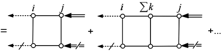
is the multiple-scattering contribution. The term ${\mathcal{S}}_{\eta \xi }^{ij}(\widehat{\mathbf{r}},\widehat{\mathbf{s}})$ corresponds to all self-contained paths starting at particle j and ending at particle i. A diagramatic illustration of the product $S_{i\eta \xi }(\widehat{\mathbf{r}},\widehat{\mathbf{s}})S_{i{\eta }^{\prime }{\xi }^{\prime }}^{\star }(\widehat{\mathbf{r}},\widehat{\mathbf{s}})$ is

$$S_{i\eta \xi }(\widehat{\mathbf{r}},\widehat{\mathbf{s}})S_{i{\eta }^{\prime }{\xi }^{\prime }}^{\star }(\widehat{\mathbf{r}},\widehat{\mathbf{s}})$$

where

$${\mathrm{e}}_{0\xi }(\widehat{\mathbf{s}}){\mathrm{e}}^{\mathrm{j}{\mathbf{K}}_0\cdot {\mathbf{R}}_{\mathrm{i}}}={}^i\Leftarrow ,\mathrm{Q}(K{\mathbf{R}}_{ij}){=}^i\text{---}{\circ }^j,$$

and

$${\mathrm{e}}^{-\mathrm{j}{\mathbf{K}}_{\mathrm{s}}\cdot {\mathbf{R}}_{\mathrm{i}}}{\mathsf{x}}_{\eta }^T(\widehat{\mathbf{r}})\mathsf{T}={\leftarrow }^i.$$

The first diagram corresponds to the single-scattering term ${\mathcal{S}}_{\eta \xi }^i(\widehat{\mathbf{r}},\widehat{\mathbf{s}}){\mathcal{S}}_{{\eta }^{\prime }{\xi }^{\prime }}^{i\star }(\widehat{\mathbf{r}},\widehat{\mathbf{s}})$, while the rest of them corresponds to the multiple-scattering term ${\mathcal{S}}_{\eta \xi }^{ij}(\widehat{\mathbf{r}},\widehat{\mathbf{s}}){\mathcal{S}}_{{\eta }^{\prime }{\xi }^{\prime }}^{ij\star }(\widehat{\mathbf{r}},\widehat{\mathbf{s}})$.

Taking the configuration average of Eq. (58) we find that the ladder quantity ${\mathcal{J}}_{\text{dL}\eta \xi {\eta }^{\prime }{\xi }^{\prime }}(\widehat{\mathbf{r}},\widehat{\mathbf{s}})$ given by Eq. (30) is (note that in the backscattering direction, κ_s = κ/ cos θ_s < 0)

$$\begin{gathered} {\mathcal{J}}_{\mathrm{dL}\eta \xi {\eta }^{\prime }{\xi }^{\prime }}(\widehat{\mathbf{r}},\widehat{\mathbf{s}})=\sum _i\langle S_{i\eta \xi }(\widehat{\mathbf{r}},\widehat{\mathbf{s}})S_{i{\eta }^{\prime }{\xi }^{\prime }}^{\star }(\widehat{\mathbf{r}},\widehat{\mathbf{s}})\rangle \\ =\frac{n_0}{k_1^2}{\mathsf{x}}_{\eta }^T(\widehat{\mathbf{r}})\mathsf{T}\left[A{\int }_0^H{\mathrm{e}}^{{\kappa }_{\mathrm{s}}{z}_i}{\mathsf{X}}_{\mathrm{L}\xi {\xi }^{\prime }}(z_i)\mathrm{d}{z}_i\right]{\mathsf{T}}^{†}{\mathsf{x}}_{{\eta }^{\prime }}^{\star }(\widehat{\mathbf{r}}), \end{gathered}$$ (62)

where the ladder correlation matrix $\mathsf{X}$_Lξξ′ (z_i), defined by

$${\mathsf{X}}_{\mathrm{L}\xi {\xi }^{\prime }}(z_i)=\langle {\mathrm{e}}_{i\xi }(\widehat{\mathbf{s}}){\mathrm{e}}_{i{\xi }^{\prime }}^{†}(\widehat{\mathbf{s}}){\rangle }_i,$$ (63)

satisfies the integral equation (compare with Eqs. (61) and (137) of Ref. [3])

$$\begin{gathered} {\mathsf{X}}_{\mathrm{L}\xi {\xi }^{\prime }}(z_i)={\mathrm{e}}^{-{\kappa }_0{z}_i}{\mathsf{E}}_{\mathrm{L}0\xi {\xi }^{\prime }}+n_0{\int }_{D-D_{2a}(z_i)}{\mathrm{e}}^{-\kappa R_{ji}}\mathsf{Q}(-k_1{\mathbf{R}}_{ji}) \\ \times {\mathsf{X}}_{\mathrm{L}\xi {\xi }^{\prime }}(z_j){\mathsf{Q}}^{†}(-k_1{\mathbf{R}}_{ji})g(R_{ji}){\mathrm{d}}^3{\mathbf{R}}_{ji}, \end{gathered}$$ (64)

with

$${\mathsf{E}}_{\mathrm{L}0\xi {\xi }^{\prime }}={\mathrm{e}}_{0\xi }(\widehat{\mathbf{s}}){\mathrm{e}}_{0{\xi }^{\prime }}^{†}(\widehat{\mathbf{s}}).$$ (65)

Recall that in Eq. (64), the domain D is a cylinder with the base area A.

If we let A → ∞, the integral equation (64) can be simplified by using the technique described in Ref. [3]. In this approach, the integral in Eq. (64) is split into two integrals according to the decomposition g(R_ji) = [g(R_ji) − 1] + 1. The first integral containing the term g(R_ji) − 1 is typical of dense media and is computed by making use of the approximation

$${\mathsf{X}}_{\mathrm{L}\xi {\xi }^{\prime }}(z_j)\approx {\mathrm{e}}^{-{\kappa }_0(z_j-z_i)}{\mathsf{X}}_{\mathrm{L}\xi {\xi }^{\prime }}(z_i),$$ (66)

while the second integral is typical of sparse media and is computed by employing the sparse-medium approximation for the integration domain, as well as the far-field representation for the radiating spherical wave functions. Note that because the function g(R_ji) − 1 tends to zero after a distance of several particle radii, the approximation (66) is local in the sense that it is valid in the vicinity of particle i (more precisely, inside a ball around particle i whose radius R₀ is determined by the interval [2a, R₀] in which the function g(R_ji) − 1 is not negligible, e.g., R₀ ≈ 8a).

In summary, the ladder reflection matrix for a layer with densely distributed particles is computed as follows:

1. solve the integral equation (64) for the ladder correlation matrix $\mathsf{X}$_Lξξ′ (z_i);

2. compute ${\mathcal{J}}_{\text{dL}\eta \xi {\eta }^{\prime }{\xi }^{\prime }}(\widehat{\mathbf{r}},\widehat{\mathbf{s}})$ from Eq. (62); and

3. compute the ladder reflection matrix ${\mathsf{R}}_{\mathrm{L}}(\widehat{\mathbf{r}},\widehat{\mathbf{s}})$ from Eq. (38), that is,

$$R_{\mathrm{L}(\eta ,{\eta }^{\prime })(\xi ,{\xi }^{\prime })}(\widehat{\mathbf{r}},\widehat{\mathbf{s}})=\frac{1}{A\cos {\theta }_0\mid \cos {\theta }_{\mathrm{s}}\mid }{\mathcal{J}}_{\mathrm{dL}\eta \xi {\eta }^{\prime }{\xi }^{\prime }}(\widehat{\mathbf{r}},\widehat{\mathbf{s}}).$$ (67)

From Eqs. (62) and (67) it is apparent that ${\mathsf{R}}_{\mathrm{L}}(\widehat{\mathbf{r}},\widehat{\mathbf{s}})$ does not depend on the illuminated area A.

Some comments can be made here.

1. In the case of transmission, the approximation (49) implies that the elements of the amplitude matrix for particle i defined by Eq. (41), are given by (compare with Eq. (51))

   $$S_{i\eta \xi }(\widehat{\mathbf{r}},\widehat{\mathbf{s}})=-\frac{\mathrm{j}}{k_1}{\mathrm{e}}^{-\mathrm{j}{\mathbf{K}}_{\mathrm{s}}\cdot {\mathbf{R}}_i}{\mathrm{e}}^{\mathrm{j}H{\mathbf{K}}_{\mathrm{s}}\cdot \widehat{\mathbf{z}}}{\mathsf{x}}_{\eta }^T(\widehat{\mathbf{r}})\mathsf{T}{\mathrm{e}}_{i\xi }(\widehat{\mathbf{s}}),\eta ,\xi =\theta ,\phi .$$ (68)
   Consequently, we get (compare with Eq. (62) and take note that in the forward scattering direction, κ_s = κ/ cos θ_s > 0)

   $$\begin{gathered} {\mathcal{J}}_{\mathrm{dL}\eta \xi {\eta }^{\prime }{\xi }^{\prime }}(\widehat{\mathbf{r}},\widehat{\mathbf{s}})=\sum _i\langle S_{i\eta \xi }(\widehat{\mathbf{r}},\widehat{\mathbf{s}})S_{i{\eta }^{\prime }{\xi }^{\prime }}^{\star }(\widehat{\mathbf{r}},\widehat{\mathbf{s}})\rangle \\ =\frac{n_0}{k_1^2}{\mathsf{x}}_{\eta }^T(\widehat{\mathbf{r}})\mathsf{T}\left[A{\int }_0^H{\mathrm{e}}^{-{\kappa }_{\mathrm{s}}(H-z_i)}{\mathsf{X}}_{\mathrm{L}\xi {\xi }^{\prime }}(z_i)\mathrm{d}{z}_i\right]{\mathsf{T}}^{†}{\mathsf{x}}_{{\eta }^{\prime }}^{\star }(\widehat{\mathbf{r}}), \end{gathered}$$ (69)

   while the elements of the ladder transmission matrix

   $${\mathsf{T}}_{\mathrm{L}}(\widehat{\mathbf{r}},\widehat{\mathbf{s}})=[T_{\mathrm{L}(\eta ,{\eta }^{\prime })(\xi ,{\xi }^{\prime })}(\widehat{\mathbf{r}},\widehat{\mathbf{s}})]$$

   are

   $$T_{\mathrm{L}(\eta ,{\eta }^{\prime })(\xi ,{\xi }^{\prime })}(\widehat{\mathbf{r}},\widehat{\mathbf{s}})=\frac{1}{A\cos {\theta }_0\mid \cos {\theta }_{\mathrm{s}}\mid }{\mathcal{J}}_{\mathrm{dL}\eta \xi {\eta }^{\prime }{\xi }^{\prime }}(\widehat{\mathbf{r}},\widehat{\mathbf{s}}).$$ (70)

   The expressions for the reflection matrix given by Eqs. (62) and (67), and for the transmission matrix given by Eqs. (69) and (70), coincide with those derived in Ref. [3]. The difference is that in the present derivation, the observation point is outside the discrete random layer.

2. In view of Eq. (59), the ladder reflection matrix can be decomposed into a single- and a multiple-scattering component,

   $${\mathsf{R}}_{\mathrm{L}}(\widehat{\mathbf{r}},\widehat{\mathbf{s}})={\mathsf{R}}_{\mathrm{L}}^1(\widehat{\mathbf{r}},\widehat{\mathbf{s}})+{\mathsf{R}}_{\mathrm{L}}^{\mathrm{M}}(\widehat{\mathbf{r}},\widehat{\mathbf{s}}),$$ (71)

   where the single-scattering component is

   $$\begin{gathered} R_{\mathrm{L}(\eta ,{\eta }^{\prime })(\xi ,{\xi }^{\prime })}^1(\widehat{\mathbf{r}},\widehat{\mathbf{s}})=\frac{1}{A\cos {\theta }_0\mid \cos {\theta }_{\mathrm{s}}\mid }{\mathcal{J}}_{\mathrm{L}\eta \xi {\eta }^{\prime }{\xi }^{\prime }}^1(\widehat{\mathbf{r}},\widehat{\mathbf{s}}) \\ =\frac{1}{A\cos {\theta }_0\mid \cos {\theta }_{\mathrm{s}}\mid }\sum _i\langle {\mathcal{S}}_{\eta \xi }^i(\widehat{\mathbf{r}},\widehat{\mathbf{s}}){\mathcal{S}}_{{\eta }^{\prime },{\xi }^{\prime }}^{i\star }(\widehat{\mathbf{r}},\widehat{\mathbf{s}})\rangle , \end{gathered}$$ (72)

   with (cf. Eq. (60))

   $$\begin{gathered} {\mathcal{J}}_{\mathrm{L}\eta \xi {\eta }^{\prime }{\xi }^{\prime }}^1(\widehat{\mathbf{r}},\widehat{\mathbf{s}})=\frac{n_0}{k_1^2}\left[A\frac{1-{\mathsf{e}}^{-({\kappa }_0-{\kappa }_{\mathrm{s}})H}}{{\kappa }_0-{\kappa }_{\mathrm{s}}}\right] \\ \times {\mathsf{x}}_{\eta }^T(\widehat{\mathbf{r}})\mathsf{T}{\mathrm{e}}_{0\xi }(\widehat{\mathbf{s}}){\mathsf{e}}_{0{\xi }^{\prime }}^{†}(\widehat{\mathbf{s}}){\mathsf{T}}^{†}{\mathsf{x}}_{{\eta }^{\prime }}^{\star }(\widehat{\mathbf{r}}), \end{gathered}$$ (73)

   while the multiple-scattering component is

$$\begin{gathered} R_{\mathrm{L}(\eta ,{\eta }^{\prime })(\xi ,{\xi }^{\prime })}^{\mathrm{M}}(\widehat{\mathbf{r}},\widehat{\mathbf{s}})=\frac{1}{A\cos {\theta }_0\mid \cos {\theta }_{\mathrm{s}}\mid }{\mathcal{J}}_{\mathrm{dL}\eta \xi {\eta }^{\prime }{\xi }^{\prime }}^{\mathrm{M}}(\widehat{\mathbf{r}},\widehat{\mathbf{s}}) \\ =\frac{1}{A\cos {\theta }_0\mid \cos {\theta }_{\mathrm{s}}\mid }\sum _i\sum _{j\ne i}\langle {\mathcal{S}}_{\eta \xi }^{ij}(\widehat{\mathbf{r}},\widehat{\mathbf{s}}){\mathcal{S}}_{{\eta }^{\prime }{\xi }^{\prime }}^{ij\star }(\widehat{\mathbf{r}},\widehat{\mathbf{s}})\rangle . \end{gathered}$$ (74)

3.1.2. Sparse medium

For sparse media, the complexity of the problem can be reduced by means of the following approach. Using the far-field representation for the matrix $\mathsf{Q}$(−k₁R_ji),

$$\mathsf{Q}(-k_1{\mathbf{R}}_{ji})=\frac{{\mathrm{e}}^{\mathrm{j}{k}_1{R}_{ji}}}{k_1{R}_{ji}}{\mathsf{Q}}_{\infty }(-{\widehat{\mathbf{R}}}_{ji}),R_{ji}\to \infty ,$$ (75)

$${\mathsf{Q}}_{\infty }(-{\widehat{\mathbf{R}}}_{ji})=-4\pi \mathrm{j}{\mathrm{x}}^{\star }(-{\widehat{\mathbf{R}}}_{ji})\cdot {\mathrm{x}}^T(-{\widehat{\mathbf{R}}}_{ji})\mathsf{T},$$ (76)

the relation ${\mathrm{e}}_{0\xi }(\widehat{\mathbf{s}})=4\pi {\mathsf{x}}_{\xi }^{\star }(\widehat{\mathbf{s}})$, and the approximation g(R_ji) ≈ 1, we find that the ladder correlation matrix $\mathsf{X}$_Lξξ′ (z_i) obeys the integral equation

$$\begin{gathered} {\mathsf{X}}_{\mathrm{L}\xi {\xi }^{\prime }}(z_i)=16{\pi }^2{\mathsf{e}}^{-{\kappa }_0{z}_i}{\mathsf{x}}_{\xi }^{\star }(\widehat{\mathbf{s}}){\mathsf{x}}_{{\xi }^{\prime }}^T(\widehat{\mathbf{s}}) \\ +16{\pi }^2\frac{n_0}{k_1^2}\sum _{{\eta }^{″},{\eta }^{‴}=\theta ,\phi }\sum _{b=\pm }{\int }_{{\Omega }_b}{\mathsf{x}}_{{\eta }^{″}}^{\star }({\widehat{\mathbf{R}}}_{ij}){\mathsf{x}}_{{\eta }^{‴}}^T({\widehat{\mathbf{R}}}_{ij}) \\ \times \left[\frac{1}{\mid \cos {\theta }_{ij}\mid }{\int }_0^H{\delta }_{b,\mathrm{sgn}(z_i-z_j)}{\mathsf{e}}^{-b\kappa \frac{z_i-z_j}{\mid \cos {\theta }_{ij}\mid }}{\mathsf{x}}_{{\eta }^{″}}^T({\widehat{\mathbf{R}}}_{ij})\mathsf{T} \\ \times {\mathsf{X}}_{\mathrm{L}\xi {\xi }^{\prime }}(z_j){\mathsf{T}}^{†}{\mathsf{x}}_{{\eta }^{‴}}^{\star }({\widehat{\mathbf{R}}}_{ij})\mathrm{d}{z}_j\right]{\mathrm{d}}^2{\widehat{\mathbf{R}}}_{ij}, \end{gathered}$$ (77)

where Ω₊ and Ω₋ are the upper and the lower unit hemispheres and δ_b,sgn(z_i−z_j) is the indicator function

$${\delta }_{b,\mathrm{sgn}(z_i-z_j)}=\{\begin{array}{cc}1,\hfill & b=\mathrm{sgn}(z_i-z_j)\hfill \\ 0,\hfill & b\ne \mathrm{sgn}(z_i-z_j)\hfill \end{array}\phantom{\}}.$$ (78)

Defining the 4 × 4 ladder matrix

$${\mathfrak{R}}_{\mathrm{L}}(z_i,\widehat{\mathbf{k}})=[{\mathfrak{R}}_{\mathrm{L}(\eta ,{\eta }^{\prime })(\xi ,{\xi }^{\prime })}(z_i,\widehat{\mathbf{k}})]$$ (79)

by

$${\mathfrak{R}}_{\mathrm{L}(\eta ,{\eta }^{\prime })(\xi ,{\xi }^{\prime })}(z_i,\widehat{\mathbf{k}})=\frac{n_0}{k_1^2}{\mathsf{x}}_{\eta }^T(\widehat{\mathbf{k}}){\mathsf{TX}}_{\mathrm{L}\xi {\xi }^{\prime }}(z_i){\mathsf{T}}^{†}{\mathsf{x}}_{{\eta }^{\prime }}^{\star }(\widehat{\mathbf{k}}),$$ (80)

and using Eq. (77) along with the relations

$${\mathsf{x}}_{\eta }^T(\widehat{\mathbf{k}}){\mathsf{Tx}}_{\xi }^{\star }({\widehat{\mathbf{k}}}^{\prime })=\mathrm{j}\frac{k_1}{4\pi }{S}_{0\eta \xi }(\widehat{\mathbf{k}},{\widehat{\mathbf{k}}}^{\prime })$$ (81)

and

$$Z_{\mathrm{JL}(\eta ,\xi )({\eta }^{\prime },{\xi }^{\prime })}(\widehat{\mathbf{k}},{\widehat{\mathbf{k}}}^{\prime })=S_{0\eta {\eta }^{\prime }}(\widehat{\mathbf{k}},{\widehat{\mathbf{k}}}^{\prime })S_{0\xi {\xi }^{\prime }}^{\star }(\widehat{\mathbf{k}},{\widehat{\mathbf{k}}}^{\prime }),$$ (82)

where $S_{0\eta \xi }(\widehat{\mathbf{k}},{\widehat{\mathbf{k}}}^{\prime })$ are the elements of the single-particle amplitude matrix in the particle-centered coordinate system and

$${\mathsf{Z}}_{\mathrm{JL}}(\widehat{\mathbf{k}},{\widehat{\mathbf{k}}}^{\prime })=[Z_{\mathrm{JL}(\eta ,\xi )({\eta }^{\prime },{\xi }^{\prime })}(\widehat{\mathbf{k}},{\widehat{\mathbf{k}}}^{\prime })]$$ (83)

is the ladder coherency phase matrix, we obtain the following integral equation for ${\mathfrak{R}}_{\mathrm{L}}(z_i,\widehat{\mathbf{k}})$xsxs:

$$\begin{gathered} {\mathfrak{R}}_{\mathrm{L}}(z_i,\widehat{\mathbf{k}})=n_0{\mathrm{e}}^{-{\kappa }_0{z}_i}{\mathsf{Z}}_{\mathrm{JL}}(\widehat{\mathbf{k}},\widehat{\mathbf{s}})+n_0\sum _{b=\pm }{\int }_{{\Omega }_b}{\mathsf{Z}}_{\mathrm{JL}}(\widehat{\mathbf{k}},{\widehat{\mathbf{R}}}_{ij}) \\ \times \left[\frac{1}{\mid \cos {\theta }_{ij}\mid }{\int }_0^H{\delta }_{b,\mathrm{sgn}(z_i-z_j)}{\mathrm{e}}^{-b\kappa \frac{z_i-z_j}{\mid \cos {\theta }_{ij}\mid }}{\mathfrak{R}}_{\mathrm{L}}(z_j,{\widehat{\mathbf{R}}}_{ij})\mathrm{d}{z}_j\right]{\mathrm{d}}^2{\widehat{\mathbf{R}}}_{ij}. \end{gathered}$$ (84)

The ladder reflection matrix ${\mathsf{R}}_{\mathrm{L}}(\widehat{\mathbf{r}},\widehat{\mathbf{s}})$ and its single-scattering component ${\mathsf{R}}_{\mathrm{L}}^1(\widehat{\mathbf{r}},\widehat{\mathbf{s}})$ are then computed as

$${\mathsf{R}}_{\mathrm{L}}(\widehat{\mathbf{r}},\widehat{\mathbf{s}})=\frac{1}{\cos {\theta }_0\mid \cos {\theta }_{\mathrm{s}}\mid }{\int }_0^H{\mathrm{e}}^{{\kappa }_{\mathrm{s}}{z}_i}{\mathfrak{R}}_{\mathrm{L}}(z_i,\widehat{\mathbf{r}})\mathrm{d}{z}_i,$$ (85)

and

$${\mathsf{R}}_{\mathrm{L}}^1(\widehat{\mathbf{r}},\widehat{\mathbf{s}})=\frac{1}{\cos {\theta }_0\mid \cos {\theta }_{\mathrm{s}}\mid }\frac{n_0}{{\kappa }_0-{\kappa }_{\mathrm{s}}}[1-{\mathrm{e}}^{-({\kappa }_0-{\kappa }_{\mathrm{s}})H}]{\mathsf{Z}}_{\mathrm{JL}}(\widehat{\mathbf{r}},\widehat{\mathbf{s}}),$$ (86)

respectively.

The integral equation (84) is similar to the integral equation (116) of Ref. [3] for the diffuse ladder specific coherency dyadic ${\overline{\Sigma }}_{\text{dL}}(z_i,\widehat{\mathbf{k}})$. In view of this analogy, Eq. (84) can be solved by employing the solution methods of the radiative transfer theory, e.g., Picard iterations in conjunction with the discrete ordinate method.

3.2. Coherent part of the scattered radiation

A method for summing up the cyclical diagrams in the case of an external observation point has been given in Refs. [19, 20]. The idea is to consider the matrix product of the exciting field coefficients ${\mathrm{e}}_{i\xi }(\widehat{\mathbf{s}}){\mathrm{e}}_{j{\xi }^{\prime }}^{†}(\widehat{\mathbf{s}})$ and apply the reciprocity principle to the series for ${\mathrm{e}}_{j{\xi }^{\prime }}^{†}(\widehat{\mathbf{s}})$; in other words, to consider a series which corresponds to a reversed propagation direction $({\mathrm{e}}_{j{\xi }^{\prime }}^{†}(\widehat{\mathbf{s}})\to {\mathrm{e}}_{j{\xi }^{\prime }}^{†}(-\widehat{\mathbf{r}}))$. Essentially, by using the reciprocity principle, the cyclical diagrams are transformed into ladder diagrams involving only pair correlation functions.

3.2.1. Dense medium

The cross quantity ${\mathcal{J}}_{\text{dC}\eta \xi {\eta }^{\prime }{\xi }^{\prime }}(\widehat{\mathbf{r}},\widehat{\mathbf{s}})$, which determines the cross reflection matrix, is associated with the interference of two waves propagating along the same self-contained path connecting particles i and j, but in opposite directions. From Eq (31), we have

$$\begin{gathered} {\mathcal{J}}_{\mathrm{dC}\eta \xi {\eta }^{\prime }{\xi }^{\prime }}(\widehat{\mathbf{r}},\widehat{\mathbf{s}})=\sum _i\sum _{j\ne i}\langle S_{i\eta \xi }(\widehat{\mathbf{r}},\widehat{\mathbf{s}})S_{j{\eta }^{\prime }{\xi }^{\prime }}^{\star }(\widehat{\mathbf{r}},\widehat{\mathbf{s}})\rangle \\ -\sum _i\sum _j\langle S_{i\eta \xi }(\widehat{\mathbf{r}},\widehat{\mathbf{s}})\rangle \langle S_{j{\eta }^{\prime }{\xi }^{\prime }}^{\star }(\widehat{\mathbf{r}},\widehat{\mathbf{s}})\rangle , \end{gathered}$$ (87)

with (cf. Eq. (10))

$$\begin{gathered} S_{i\eta \xi }(\widehat{\mathbf{r}},\widehat{\mathbf{s}})S_{j{\eta }^{\prime }{\xi }^{\prime }}^{\star }(\widehat{\mathbf{r}},\widehat{\mathbf{s}}) \\ =\frac{1}{k_1^2}\left[{\mathrm{e}}^{-\mathrm{j}{k}_1\widehat{\mathbf{r}}\cdot {\mathbf{R}}_i}{\mathsf{x}}_{\eta }^T(\widehat{\mathbf{r}}){\mathsf{Te}}_{i\xi }(\widehat{\mathbf{s}})\right]{\left[{\mathrm{e}}^{-\mathrm{j}{k}_1\widehat{\mathbf{r}}\cdot {\mathbf{R}}_j}{\mathsf{x}}_{{\eta }^{\prime }}^T(\widehat{\mathbf{r}}){\mathsf{Te}}_{i{\xi }^{\prime }}(\widehat{\mathbf{s}})\right]}^{\star } \\ =\frac{1}{k_1^2}{\mathrm{e}}^{-\mathrm{j}{k}_1\widehat{\mathbf{r}}\cdot {\mathbf{R}}_i}{\mathsf{x}}_{\eta }^T(\widehat{\mathbf{r}}){\mathsf{Te}}_{i\xi }(\widehat{\mathbf{s}}){\mathsf{e}}_{j{\xi }^{\prime }}^{†}(\widehat{\mathbf{s}}){\mathsf{T}}^{†}{\mathsf{x}}_{{\eta }^{\prime }}^{\star }(\widehat{\mathbf{r}}){\mathsf{e}}^{\mathrm{j}{k}_1\widehat{\mathbf{r}}\cdot {\mathbf{R}}_i}. \end{gathered}$$ (88)

For the time being, in Eq. (88) and in what follows, we use the free-space quantities $k_1\widehat{\mathbf{s}}$, $k_1\widehat{\mathbf{r}}$, and $\mathsf{Q}$(k₁·) instead of K₀, K_s, and $\mathsf{Q}$(K·), respectively; they will be replaced with the effective-medium quantities just before taking the configuration average. The derivation involves the following steps.

Step 1. Using the series representations for ${\mathrm{e}}_{i\xi }(\widehat{\mathbf{s}})$ and ${\mathrm{e}}_{j{\xi }^{\prime }}^{†}(\widehat{\mathbf{s}})$ as given by Eq. (54) with ${\mathrm{e}}_{0i\xi }(\widehat{\mathbf{s}})=\text{exp}(\mathrm{j}{k}_1\widehat{\mathbf{s}}\cdot {\mathbf{R}}_i){\mathrm{e}}_{0\xi }(\widehat{\mathbf{s}})$, and retaining in the matrix product ${\mathrm{e}}_{i\xi }(\widehat{\mathbf{s}}){\mathrm{e}}_{j{\xi }^{\prime }}^{†}(\widehat{\mathbf{s}})$ only the terms corresponding to the cyclical diagrams, we obtain

$$\begin{gathered} {\mathsf{e}}_{i\xi }(\widehat{\mathbf{s}}){\mathsf{e}}_{j{\xi }^{\prime }}^{†}(\widehat{\mathbf{s}})=\left[{\mathrm{e}}_{0\xi }(\widehat{\mathbf{s}}){\mathsf{e}}^{\mathrm{j}{k}_1\widehat{\mathbf{s}}\cdot {\mathbf{R}}_i}\right]{\left[{\mathrm{e}}_{0{\xi }^{\prime }}(\widehat{\mathbf{s}}){\mathsf{e}}^{\mathrm{j}{k}_1\widehat{\mathbf{s}}\cdot {\mathbf{R}}_j}\right]}^{†} \\ +\left[\mathsf{Q}(k_1{\mathbf{R}}_{ij}){\mathrm{e}}_{0\xi }(\widehat{\mathbf{s}}){\mathsf{e}}^{\mathrm{j}{k}_1\widehat{\mathbf{s}}\cdot {\mathbf{R}}_j}\right]{\left[\mathsf{Q}(k_1{\mathbf{R}}_{ji}){\mathrm{e}}_{0{\xi }^{\prime }}(\widehat{\mathbf{s}}){\mathsf{e}}^{\mathrm{j}{k}_1\widehat{\mathbf{s}}\cdot {\mathbf{R}}_i}\right]}^{†} \\ +\sum _{k\ne i,j}\left[\mathsf{Q}(k_1{\mathbf{R}}_{ik})\mathsf{Q}(k_1{\mathbf{R}}_{kj}){\mathrm{e}}_{0\xi }(\widehat{\mathbf{s}}){\mathsf{e}}^{\mathrm{j}{k}_1\widehat{\mathbf{s}}\cdot {\mathbf{R}}_j}\right] \\ \times {\left[\mathsf{Q}(k_1{\mathbf{R}}_{jk})\mathsf{Q}(k_1{\mathbf{R}}_{ki}){\mathrm{e}}_{0{\xi }^{\prime }}(\widehat{\mathbf{s}}){\mathsf{e}}^{\mathrm{j}{k}_1\widehat{\mathbf{s}}\cdot {\mathbf{R}}_i}\right]}^{†}+\cdots . \end{gathered}$$ (89)

Inserting Eq. (89) in Eq. (88), we find (compare with Eq. (59))

$$S_{i\eta \xi }(\widehat{\mathbf{r}},\widehat{\mathbf{s}})S_{j{\eta }^{\prime }{\xi }^{\prime }}^{\star }(\widehat{\mathbf{r}},\widehat{\mathbf{s}})={\mathcal{S}}_{\eta \xi }^i(\widehat{\mathbf{r}},\widehat{\mathbf{s}}){\mathcal{S}}_{{\eta }^{\prime }{\xi }^{\prime }}^{j\star }(\widehat{\mathbf{r}},\widehat{\mathbf{s}})+{\mathcal{S}}_{\eta \xi }^{ij}(\widehat{\mathbf{r}},\widehat{\mathbf{s}}){\mathcal{S}}_{{\eta }^{\prime }{\xi }^{\prime }}^{ji\star }(\widehat{\mathbf{r}},\widehat{\mathbf{s}}),$$ (90)

with

$$\begin{gathered} {\mathcal{S}}_{\eta \xi }^i(\widehat{\mathbf{r}},\widehat{\mathbf{s}}){\mathcal{S}}_{{\eta }^{\prime }{\xi }^{\prime }}^{j\star }(\widehat{\mathbf{r}},\widehat{\mathbf{s}})=\frac{1}{k_1^2}\left[{\mathsf{e}}^{-\mathrm{j}{k}_1\widehat{\mathbf{r}}\cdot {\mathbf{R}}_i}{\mathsf{x}}_{\eta }^T(\widehat{\mathbf{r}}){\mathsf{Te}}_{0\xi }(\widehat{\mathbf{s}}){\mathsf{e}}^{\mathrm{j}{k}_1\widehat{\mathbf{s}}\cdot {\mathbf{R}}_i}\right] \\ \times {\left[{\mathsf{e}}^{-\mathrm{j}{k}_1\widehat{\mathbf{r}}\cdot {\mathbf{R}}_j}{\mathsf{x}}_{{\eta }^{\prime }}^T(\widehat{\mathbf{r}}){\mathsf{Te}}_{0{\xi }^{\prime }}(\widehat{\mathbf{s}}){\mathsf{e}}^{\mathrm{j}{k}_1\widehat{\mathbf{s}}\cdot {\mathbf{R}}_j}\right]}^{\star } \end{gathered}$$ (91)

and

$$\begin{gathered} {\mathcal{S}}_{\eta \xi }^{ij}(\widehat{\mathbf{r}},\widehat{\mathbf{s}}){\mathcal{S}}_{{\eta }^{\prime }{\xi }^{\prime }}^{ji\star }(\widehat{\mathbf{r}},\widehat{\mathbf{s}}) \\ =\frac{1}{k_1^2}\left[{\mathsf{e}}^{-\mathrm{j}{k}_1\widehat{\mathbf{r}}\cdot {\mathbf{R}}_i}{\mathsf{x}}_{\eta }^T(\widehat{\mathbf{r}})\mathsf{TQ}(k_1{\mathbf{R}}_{ij}){\mathsf{e}}_{0\xi }(\widehat{\mathbf{s}}){\mathsf{e}}^{\mathrm{j}{k}_1\widehat{\mathbf{s}}\cdot {\mathbf{R}}_j}\right] \\ \times {\left[{\mathsf{e}}^{-\mathrm{j}{k}_1\widehat{\mathbf{r}}\cdot {\mathbf{R}}_j}{\mathsf{x}}_{{\eta }^{\prime }}^T(\widehat{\mathbf{r}})\mathsf{TQ}(k_1{\mathbf{R}}_{ji}){\mathsf{e}}_{0{\xi }^{\prime }}(\widehat{\mathbf{s}}){\mathsf{e}}^{\mathrm{j}{k}_1\widehat{\mathbf{s}}\cdot {\mathbf{R}}_i}\right]}^{\star } \\ +\frac{1}{k_1^2}\sum _{k\ne i,j}\left[{\mathsf{e}}^{-\mathrm{j}{k}_1\widehat{\mathbf{r}}\cdot {\mathbf{R}}_i}{\mathsf{x}}_{\eta }^T(\widehat{\mathbf{r}})\mathsf{TQ}(k_1{\mathbf{R}}_{ik})\mathsf{Q}(k_1{\mathbf{R}}_{kj}){\mathsf{e}}_{0\xi }(\widehat{\mathbf{s}}){\mathsf{e}}^{\mathrm{j}{k}_1\widehat{\mathbf{s}}\cdot {\mathbf{R}}_j}\right] \\ \times {\left[{\mathsf{e}}^{-\mathrm{j}{k}_1\widehat{\mathbf{r}}\cdot {\mathbf{R}}_j}{\mathsf{x}}_{{\eta }^{\prime }}^T(\widehat{\mathbf{r}})\mathsf{TQ}(k_1{\mathbf{R}}_{jk})\mathsf{Q}(k_1{\mathbf{R}}_{ki}){\mathsf{e}}_{0{\xi }^{\prime }}(\widehat{\mathbf{s}}){\mathsf{e}}^{\mathrm{j}{k}_1\widehat{\mathbf{s}}\cdot {\mathbf{R}}_i}\right]}^{\star }+\cdots . \end{gathered}$$ (92)

In a diagramatic representation, the product ${\mathcal{S}}_{\eta \xi }^{ij}(\widehat{\mathbf{r}},\widehat{\mathbf{s}}){\mathcal{S}}_{{\eta }^{\prime }{\xi }^{\prime }}^{ji\star }(\widehat{\mathbf{r}},\widehat{\mathbf{s}})$ is illustrated as

$${\mathcal{S}}_{\eta \xi }^{ij}(\widehat{\mathbf{r}},\widehat{\mathbf{s}}){\mathcal{S}}_{{\eta }^{\prime }{\xi }^{\prime }}^{ji\star }(\widehat{\mathbf{r}},\widehat{\mathbf{s}})$$

where

$${\mathrm{e}}_{0\xi }(\widehat{\mathbf{s}}){\mathrm{e}}^{\mathrm{j}{k}_1\widehat{\mathbf{s}}\cdot {\mathbf{R}}_j}={}^j\Leftarrow ,\mathrm{Q}(k_1{\mathbf{R}}_{ij})={}^i\text{---}{\circ }^j,$$

and

$${\mathrm{e}}^{-\mathrm{j}{k}_1\widehat{\mathbf{r}}\cdot {\mathbf{R}}_i}{\mathsf{x}}_{\eta }^T(\widehat{\mathbf{r}})\mathsf{T}={\leftarrow }^i.$$

Step 2. Consider the single-scattering term ${\mathcal{S}}_{\eta \xi }^i(\widehat{\mathbf{r}},\widehat{\mathbf{s}}){\mathcal{S}}_{{\eta }^{\prime }{\xi }^{\prime }}^{j\star }(\widehat{\mathbf{r}},\widehat{\mathbf{s}})$ given by Eq. (91). Replacing $k_1\widehat{\mathbf{s}}$ and $k_1\widehat{\mathbf{r}}$ by K₀ and K_s, respectively, taking the configuration average, and combining the resulting expression with the coherent term ${\sum }_i{\sum }_j\langle S_{i\eta \xi }(\widehat{\mathbf{r}},\widehat{\mathbf{s}})\rangle \langle S_{j{\eta }^{\prime }{\xi }^{\prime }}^{\star }(\widehat{\mathbf{r}},\widehat{\mathbf{s}})\rangle$ gives the following contribution to ${\mathcal{J}}_{\text{dC}\eta \xi {\eta }^{\prime }{\xi }^{\prime }}(\widehat{\mathbf{r}},\widehat{\mathbf{s}})$ in Eq. (87) (R_ji = R_j − R_i):

$$\begin{gathered} \sum _i\sum _{j\ne i}\langle {\mathcal{S}}_{\eta \xi }^i(\widehat{\mathbf{r}},\widehat{\mathbf{s}}){\mathcal{S}}_{{\eta }^{\prime }{\xi }^{\prime }}^{j\star }(\widehat{\mathbf{r}},\widehat{\mathbf{s}})\rangle -\sum _i\sum _j\langle S_{i\eta \xi }(\widehat{\mathbf{r}},\widehat{\mathbf{s}})\rangle \langle S_{j{\eta }^{\prime }{\xi }^{\prime }}^{\star }(\widehat{\mathbf{r}},\widehat{\mathbf{s}})\rangle \\ =\frac{n_0^2}{k_1^2}A{\int }_0^H{\mathsf{e}}^{-({\kappa }_0-{\kappa }_{\mathrm{s}})z_i}\left\{{\int }_D{\mathsf{e}}^{-\mathrm{j}({\mathbf{K}}_0^{\star }-{\mathbf{K}}_{\mathrm{s}}^{\star })\cdot {\mathbf{R}}_{ji}}[g(R_{ji})-1]{\mathrm{d}}^3{\mathbf{R}}_{ji}\right\}\mathrm{d}{z}_i \\ \times {\mathsf{x}}_{\eta }^T(\widehat{\mathbf{r}}){\mathsf{Te}}_{0\xi }(\widehat{\mathbf{s}}){\mathsf{e}}_{0{\xi }^{\prime }}^{†}(\widehat{\mathbf{s}}){\mathsf{T}}^{†}{\mathsf{x}}_{{\eta }^{\prime }}^{\star }(\widehat{\mathbf{r}}). \end{gathered}$$ (93)

For sparse media, we have g(R_ji) = 1, implying

$$\sum _i\sum _{j\ne i}\langle {\mathcal{S}}_{\eta \xi }^i(\widehat{\mathbf{r}},\widehat{\mathbf{s}}){\mathcal{S}}_{{\eta }^{\prime }{\xi }^{\prime }}^{j\star }(\widehat{\mathbf{r}},\widehat{\mathbf{s}})\rangle =\sum _i\sum _j\langle S_{i\eta \xi }(\widehat{\mathbf{r}},\widehat{\mathbf{s}})\rangle \langle S_{j{\eta }^{\prime }{\xi }^{\prime }}^{\star }(\widehat{\mathbf{r}},\widehat{\mathbf{s}})\rangle .$$

Thus, when taking the configuration average, the contribution of the single-scattering term ${\sum }_i{\sum }_{j\ne i}\langle {\mathcal{S}}_{\eta \xi }^i(\widehat{\mathbf{r}},\widehat{\mathbf{s}}){\mathcal{S}}_{{\eta }^{\prime }{\xi }^{\prime }}^{j\star }(\widehat{\mathbf{r}},\widehat{\mathbf{s}})\rangle$ is canceled by the contribution of the coherent term ${\sum }_i{\sum }_j\langle S_{i\eta \xi }(\widehat{\mathbf{r}},\widehat{\mathbf{s}})\rangle \langle S_{j{\eta }^{\prime }{\xi }^{\prime }}^{\star }(\widehat{\mathbf{r}},\widehat{\mathbf{s}})\rangle$. Adopting this sparse-medium simplification in Eqs. (87) and (90), we compute ${\mathcal{J}}_{\text{dC}\eta \xi {\eta }^{\prime }{\xi }^{\prime }}(\widehat{\mathbf{r}},\widehat{\mathbf{s}})$ by means of the relation

$${\mathcal{J}}_{\mathrm{dC}\eta \xi {\eta }^{\prime }{\xi }^{\prime }}(\widehat{\mathbf{r}},\widehat{\mathbf{s}})=\sum _i\sum _{j\ne i}\langle {\mathcal{S}}_{\eta \xi }^{ij}(\widehat{\mathbf{r}},\widehat{\mathbf{s}}){\mathcal{S}}_{{\eta }^{\prime }{\xi }^{\prime }}^{ji\star }(\widehat{\mathbf{r}},\widehat{\mathbf{s}})\rangle$$ (94)

with ${\mathcal{S}}_{\eta \xi }^{ij}(\widehat{\mathbf{r}},\widehat{\mathbf{s}}){\mathcal{S}}_{{\eta }^{\prime }{\xi }^{\prime }}^{ji\star }(\widehat{\mathbf{r}},\widehat{\mathbf{s}})$ as in Eq. (92).

Step 3. Using the symmetry relation for the ξ-polarized vector of spherical harmonics (cf. Eq. (12) of Ref. [1])

$${\mathsf{x}}_{\xi mn}^{\star }(-\widehat{\mathbf{r}})=h_{\xi }{\mathsf{x}}_{\xi -mn}(\widehat{\mathbf{r}}),$$

where h_ξ is the indicator function

$$h_{\xi }=\{\begin{array}{cc}1,\hfill & \xi =\theta \hfill \\ -1,\hfill & \xi =\phi \hfill \end{array}\phantom{\}},$$

as well as the symmetry relation for the translation matrix (cf. Eq. (23) of Ref. [1])

$${\mathcal{T}}_{mn,m_1{n}_1}^{31}(k_1{\mathbf{R}}_{ji})={\mathcal{T}}_{-m_1{n}_1,-mn}^{31}(k_1{\mathbf{R}}_{ij}),{\mathbf{R}}_{ij}=-{\mathbf{R}}_{ji},$$

we transform the series for ${\mathcal{S}}_{{\eta }^{\prime }{\xi }^{\prime }}^{ji\star }(\widehat{\mathbf{r}},\widehat{\mathbf{s}})$ in Eq. (92) according to the reciprocity principle. Specifically, each term in the series for ${\mathcal{S}}_{{\eta }^{\prime }{\xi }^{\prime }}^{ji\star }(\widehat{\mathbf{r}},\widehat{\mathbf{s}})$ is transformed by using the basic result

$${\mathsf{x}}_{{\eta }^{\prime }}^T(\widehat{\mathbf{r}})\mathsf{TQ}(k_1{\mathbf{R}}_{ji}){\mathrm{e}}_{{\xi }^{\prime }}(\widehat{\mathbf{s}})=h_{{\eta }^{\prime }}{h}_{{\xi }^{\prime }}{\mathsf{x}}_{{\xi }^{\prime }}^T(-\widehat{\mathbf{s}})\mathsf{TQ}(k_1{\mathbf{R}}_{ji}){\mathrm{e}}_{{\eta }^{\prime }}(-\widehat{\mathbf{r}}),$$

which follows from the representation ${\mathrm{e}}_{0{\xi }^{\prime }}(\widehat{\mathbf{s}})=4\pi {\mathsf{x}}_{{\xi }^{\prime }}^{\star }(\widehat{\mathbf{s}})$, the relation $\mathsf{Q}(k_1{\mathbf{R}}_{ji})={\mathcal{T}}_{31}^T(k_1{\mathbf{R}}_{ji})\mathsf{T}$, the identity (note that for spherical particles, $\mathsf{T}$ is a diagonal matrix)

$${\mathsf{x}}_{{\eta }^{\prime }}^T(\widehat{\mathbf{r}})\mathsf{TQ}(k_1{\mathbf{R}}_{ji}){\mathsf{x}}_{{\xi }^{\prime }}^{\star }(\widehat{\mathbf{s}})={\mathsf{x}}_{{\xi }^{\prime }}^{†}(\widehat{\mathbf{s}})\mathsf{T}{\mathcal{T}}_{31}(k_1{\mathbf{R}}_{ji}){\mathsf{Tx}}_{{\eta }^{\prime }}(\widehat{\mathbf{r}}),$$

and the symmetry relation

$$\begin{gathered} \sum _{mn{m}_1{n}_1}{\mathsf{x}}_{{\xi }^{\prime }mn}^{\star }(\widehat{\mathbf{s}})T_n{\mathcal{T}}_{mn,m_1{n}_1}^{31}(k_1{\mathbf{R}}_{ji})T_{n_1}{\mathsf{x}}_{{\eta }^{\prime }}{m}_1{n}_1(\widehat{\mathbf{r}}) \\ =h_{{\eta }^{\prime }}{h}_{{\xi }^{\prime }}\sum _{mn{m}_1{n}_1}{\mathsf{x}}_{{\xi }^{\prime }-mn}(-\widehat{\mathbf{s}})T_n{\mathcal{T}}_{-m_1{n}_1,-mn}^{31}(k_1{\mathbf{R}}_{ij})T_{n_1}{\mathsf{x}}_{{\eta }^{\prime }-m_1{n}_1}^{\star }(-\widehat{\mathbf{r}}) \\ =h_{{\eta }^{\prime }}{h}_{{\xi }^{\prime }}\sum _{mn{m}_1{n}_1}{\mathsf{x}}_{{\xi }^{\prime }mn}(-\widehat{\mathbf{s}})T_n{\mathcal{T}}_{m_1{n}_1,mn}^{31}(k_1{\mathbf{R}}_{ij})T_{n_1}{\mathsf{x}}_{{\eta }^{\prime }{m}_1{n}_1}^{\star }(-\widehat{\mathbf{r}}). \end{gathered}$$

Summing over j in Eq. (92) yields an expansion in which the wave propagation direction in the series for ${\mathcal{S}}_{{\eta }^{\prime }{\xi }^{\prime }}^{ji\star }(\widehat{\mathbf{r}},\widehat{\mathbf{s}})$ is reversed; the result is

$$\begin{gathered} \sum _{j\ne i}{\mathcal{S}}_{\eta \xi }^{ij}(\widehat{\mathbf{r}},\widehat{\mathbf{s}}){\mathcal{S}}_{{\eta }^{\prime }{\xi }^{\prime }}^{ji\star }(\widehat{\mathbf{r}},\widehat{\mathbf{s}}) \\ =h_{{\eta }^{\prime }}{h}_{{\xi }^{\prime }}\left\{\frac{1}{k_1^2}\sum _{j\ne i}\left[{\mathsf{e}}^{-\mathrm{j}{k}_1\widehat{\mathbf{r}}\cdot {\mathbf{R}}_i}{\mathsf{x}}_{\eta }^T(\widehat{\mathbf{r}})\mathsf{TQ}(k_1{\mathbf{R}}_{ij}){\mathsf{e}}_{0\xi }(\widehat{\mathbf{s}}){\mathsf{e}}^{\mathrm{j}{k}_1\widehat{\mathbf{s}}\cdot {\mathbf{R}}_j}\right] \\ \times {\left[{\mathsf{e}}^{-\mathrm{j}{k}_1(-\widehat{\mathbf{s}})\cdot {\mathbf{R}}_i}{\mathsf{x}}_{{\xi }^{\prime }}^T(-\widehat{\mathbf{s}})\mathsf{TQ}(k_1{\mathbf{R}}_{ij}){\mathsf{e}}_{0{\eta }^{\prime }}(-\widehat{\mathbf{r}}){\mathsf{e}}^{\mathrm{j}{k}_1(-\widehat{\mathbf{r}})\cdot {\mathbf{R}}_j}\right]}^{\star } \\ +\frac{1}{k_1^2}\sum _{j\ne i}\sum _{k\ne i,j}\left[{\mathsf{e}}^{-\mathrm{j}{k}_1\widehat{\mathbf{r}}\cdot {\mathbf{R}}_i}{\mathsf{x}}_{\eta }^T(\widehat{\mathbf{r}})\mathsf{TQ}(k_1{\mathbf{R}}_{ik}) \\ \times \mathsf{Q}(k_1{\mathbf{R}}_{kj}){\mathsf{e}}_{0\xi }(\widehat{\mathbf{s}}){\mathsf{e}}^{\mathrm{j}{k}_1\widehat{\mathbf{s}}\cdot {\mathbf{R}}_j}\right]{\left[{\mathsf{e}}^{-\mathrm{j}{k}_1(-\widehat{\mathbf{s}})\cdot {\mathbf{R}}_i}{\mathsf{x}}_{{\xi }^{\prime }}^T(-\widehat{\mathbf{s}})\mathsf{TQ}(k_1{\mathbf{R}}_{ik}) \\ \times \mathsf{Q}(k_1{\mathbf{R}}_{kj}){\mathsf{e}}_{0{\eta }^{\prime }}(-\widehat{\mathbf{r}}){\mathsf{e}}^{\mathrm{j}{k}_1(-\widehat{\mathbf{r}})\cdot {\mathbf{R}}_j}\right]}^{\star }+\cdots \right\}. \end{gathered}$$ (95)

Step 4. On the other hand, using Eq. (10) we form the product

$$\begin{gathered} S_{i\eta \xi }(\widehat{\mathbf{r}},\widehat{\mathbf{s}})S_{i{\xi }^{\prime }{\eta }^{\prime }}^{\star }(-\widehat{\mathbf{s}},-\widehat{\mathbf{r}}) \\ =\frac{1}{k_1^2}\left[{\mathsf{e}}^{-\mathrm{j}{k}_1\widehat{\mathbf{r}}\cdot {\mathbf{R}}_i}{\mathsf{x}}_{\eta }^T(\widehat{\mathbf{r}}){\mathsf{Te}}_{i\xi }(\widehat{\mathbf{s}})\right]{\left[{\mathsf{e}}^{-\mathrm{j}{k}_1(-\widehat{\mathbf{s}})\cdot {\mathbf{R}}_i}{\mathsf{x}}_{{\xi }^{\prime }}^T(-\widehat{\mathbf{s}}){\mathsf{Te}}_{i{\eta }^{\prime }}(-\widehat{\mathbf{r}})\right]}^{\star } \\ =\frac{1}{k_1^2}{\mathsf{e}}^{-\mathrm{j}{k}_1\widehat{\mathbf{r}}\cdot {\mathbf{R}}_i}{\mathsf{x}}_{\eta }^T(\widehat{\mathbf{r}}){\mathsf{Te}}_{i\xi }(\widehat{\mathbf{s}}){\mathsf{e}}_{i{\eta }^{\prime }}^{†}(-\widehat{\mathbf{r}}){\mathsf{T}}^{†}{\mathsf{x}}_{{\xi }^{\prime }}^{\star }(-\widehat{\mathbf{s}}){\mathsf{e}}^{\mathrm{j}{k}_1(-\widehat{\mathbf{s}})\cdot {\mathbf{R}}_i}. \end{gathered}$$ (96)

By taking into account the series representations for ${\mathrm{e}}_{i\xi }(\widehat{\mathbf{s}})$ and ${\mathrm{e}}_{i{\eta }^{\prime }}^{†}(-\widehat{\mathbf{r}})$ given by Eq. (54), we retain in the matrix product ${\mathrm{e}}_{i\xi }(\widehat{\mathbf{s}}){\mathrm{e}}_{i{\eta }^{\prime }}^{†}(-\widehat{\mathbf{r}})$ only the terms corresponding to the ladder diagrams, that is,

$$\begin{gathered} {\mathsf{e}}_{i\xi }(\widehat{\mathbf{s}}){\mathsf{e}}_{i{\eta }^{\prime }}^{†}(-\widehat{\mathbf{r}}) \\ =\left[{\mathsf{e}}_{0\xi }(\widehat{\mathbf{s}}){\mathsf{e}}^{\mathrm{j}{k}_1\widehat{\mathbf{s}}\cdot {\mathbf{R}}_i}\right]{\left[{\mathsf{e}}_{0{\eta }^{\prime }}(-\widehat{\mathbf{r}}){\mathsf{e}}^{\mathrm{j}{k}_1(-\widehat{\mathbf{r}})\cdot {\mathbf{R}}_i}\right]}^{†} \\ +\sum _{j\ne i}\left[\mathsf{Q}(k_1{\mathbf{R}}_{ij}){\mathsf{e}}_{0\xi }(\widehat{\mathbf{s}}){\mathsf{e}}^{\mathrm{j}{k}_1\widehat{\mathbf{s}}\cdot {\mathbf{R}}_j}\right]{\left[\mathsf{Q}(k_1{\mathbf{R}}_{ij}){\mathsf{e}}_{0{\eta }^{\prime }}(-\widehat{\mathbf{r}}){\mathsf{e}}^{\mathrm{j}{k}_1(-\widehat{\mathbf{r}})\cdot {\mathbf{R}}_j}\right]}^{†} \\ +\sum _{j\ne i}\sum _{k\ne i,j}\left[\mathsf{Q}(k_1{\mathbf{R}}_{ik})\mathsf{Q}(k_1{\mathbf{R}}_{kj}){\mathsf{e}}_{0\xi }(\widehat{\mathbf{s}}){\mathsf{e}}^{\mathrm{j}{k}_1\widehat{\mathbf{s}}\cdot {\mathbf{R}}_j}\right] \\ \times {\left[\mathsf{Q}(k_1{\mathbf{R}}_{ik})\mathsf{Q}(k_1{\mathbf{R}}_{kj}){\mathsf{e}}_{0{\eta }^{\prime }}(-\widehat{\mathbf{r}}){\mathsf{e}}^{-\mathrm{j}{k}_1(-\widehat{\mathbf{r}})\cdot {\mathbf{R}}_j}\right]}^{†}+\cdots . \end{gathered}$$ (97)

By analogy with Eq. (57), the above series representation implies that the matrix ${\mathrm{e}}_{i\xi }(\widehat{\mathbf{s}}){\mathrm{e}}_{i{\eta }^{\prime }}^{†}(-\widehat{\mathbf{r}})$ satisfies the system of equations

$$\begin{gathered} {\mathrm{e}}_{i\xi }(\widehat{\mathbf{s}}){\mathrm{e}}_{i{\eta }^{\prime }}^{†}(-\widehat{\mathbf{r}})=\left[{\mathrm{e}}_{0\xi }(\widehat{\mathbf{s}}){\mathrm{e}}^{\mathrm{j}{k}_1\widehat{\mathbf{s}}\cdot {\mathbf{R}}_i}\right]{\left[{\mathrm{e}}_{0{\eta }^{\prime }}(-\widehat{\mathbf{r}}){\mathrm{e}}^{\mathrm{j}{k}_1(-\widehat{\mathbf{r}})\cdot {\mathbf{R}}_i}\right]}^{†} \\ +\sum _{j\ne i}[\mathsf{Q}(k_1{\mathbf{R}}_{ij}){\mathrm{e}}_{j\xi }(\widehat{\mathbf{s}})][\mathsf{Q}(k_1{\mathbf{R}}_{ij}){\mathrm{e}}_{j{\eta }^{\prime }}(-\widehat{\mathbf{r}}){]}^{†}. \end{gathered}$$ (98)

Substituting Eq. (97) in Eq. (96) gives

$$\begin{gathered} S_{i\eta \xi }(\widehat{\mathbf{r}},\widehat{\mathbf{s}})S_{i{\xi }^{\prime }{\eta }^{\prime }}^{\star }(-\widehat{\mathbf{s}},-\widehat{\mathbf{r}})={\mathcal{S}}_{\eta \xi }^i(\widehat{\mathbf{r}},\widehat{\mathbf{s}}){\mathcal{S}}_{{\xi }^{\prime }{\eta }^{\prime }}^{i\star }(-\widehat{\mathbf{s}},-\widehat{\mathbf{r}}) \\ +\sum _{j\ne i}{\mathcal{S}}_{\eta \xi }^{ij}(\widehat{\mathbf{r}},\widehat{\mathbf{s}}){\mathcal{S}}_{{\xi }^{\prime }{\eta }^{\prime }}^{ij\star }(-\widehat{\mathbf{s}},-\widehat{\mathbf{r}}), \end{gathered}$$ (99)

with (compare with Eq. (60))

$$\begin{gathered} {\mathcal{S}}_{\eta \xi }^i(\widehat{\mathbf{r}},\widehat{\mathbf{s}}){\mathcal{S}}_{{\xi }^{\prime }{\eta }^{\prime }}^{i\star }(-\widehat{\mathbf{s}},-\widehat{\mathbf{r}})=\frac{1}{k_1^2}\left[{\mathsf{e}}^{-\mathrm{j}{k}_1\widehat{\mathbf{r}}\cdot {\mathbf{R}}_i}{\mathsf{x}}_{\eta }^T(\widehat{\mathbf{r}}){\mathsf{Te}}_{0\xi }(\widehat{\mathbf{s}}){\mathsf{e}}^{\mathrm{j}{k}_1\widehat{\mathbf{s}}\cdot {\mathbf{R}}_i}\right] \\ \times {\left[{\mathsf{e}}^{-\mathrm{j}{k}_1(-\widehat{\mathbf{s}})\cdot {\mathbf{R}}_i}{\mathsf{x}}_{{\xi }^{\prime }}^T(-\widehat{\mathbf{s}}){\mathsf{Te}}_{0{\eta }^{\prime }}(-\widehat{\mathbf{r}}){\mathsf{e}}^{\mathrm{j}{k}_1(-\widehat{\mathbf{r}})\cdot {\mathbf{R}}_i}\right]}^{\star } \end{gathered}$$ (100)

and (compare with Eq. (61))

$$\begin{gathered} \sum _{j\ne i}{\mathcal{S}}_{\eta \xi }^{ij}(\widehat{\mathbf{r}},\widehat{\mathbf{s}}){\mathcal{S}}_{{\xi }^{\prime }{\eta }^{\prime }}^{ij\star }(-\widehat{\mathbf{s}},-\widehat{\mathbf{r}}) \\ =\frac{1}{k_1^2}\sum _{j\ne i}\left[{\mathsf{e}}^{-\mathrm{j}{k}_1\widehat{\mathbf{r}}\cdot {\mathbf{R}}_i}{\mathsf{x}}_{\eta }^T(\widehat{\mathbf{r}})\mathsf{TQ}(k_1{\mathbf{R}}_{ij}){\mathsf{e}}_{0\xi }(\widehat{\mathbf{s}}){\mathsf{e}}^{\mathrm{j}{k}_1\widehat{\mathbf{s}}\cdot {\mathbf{R}}_j}\right] \\ \times {\left[{\mathsf{e}}^{-\mathrm{j}{k}_1(-\widehat{\mathbf{s}})\cdot {\mathbf{R}}_i}{\mathsf{x}}_{{\xi }^{\prime }}^T(-\widehat{\mathbf{s}})\mathsf{TQ}(k_1{\mathbf{R}}_{ij}){\mathsf{e}}_{0{\eta }^{\prime }}(-\widehat{\mathbf{r}}){\mathsf{e}}^{\mathrm{j}{k}_1(-\widehat{\mathbf{r}})\cdot {\mathbf{R}}_j}\right]}^{\star }+\frac{1}{k_1^2}\sum _{j\ne i}\sum _{k\ne i,j}\left[{\mathsf{e}}^{-\mathrm{j}{k}_1\widehat{\mathbf{r}}\cdot {\mathbf{R}}_i}{\mathsf{x}}_{\eta }^T(\widehat{\mathbf{r}})\mathsf{TQ}(k_1{\mathbf{R}}_{ik}) \\ \times \mathsf{Q}(k_1{\mathbf{R}}_{kj}){\mathsf{e}}_{0\xi }(\widehat{\mathbf{s}}){\mathsf{e}}^{\mathrm{j}{k}_1\widehat{\mathbf{s}}\cdot {\mathbf{R}}_j}\right]{\left[{\mathsf{e}}^{-\mathrm{j}{k}_1(-\widehat{\mathbf{s}})\cdot {\mathbf{R}}_i}{\mathsf{x}}_{{\xi }^{\prime }}^T(-\widehat{\mathbf{s}})\mathsf{TQ}(k_1{\mathbf{R}}_{ik}) \\ \mathsf{Q}(k_1{\mathbf{R}}_{kj}){\mathsf{e}}_{0{\eta }^{\prime }}(-\widehat{\mathbf{r}}){\mathsf{e}}^{\mathrm{j}{k}_1(-\widehat{\mathbf{r}})\cdot {\mathbf{R}}_j}\right]}^{\star }+\cdots . \end{gathered}$$ (101)

A diagramatic illustration of the product ${\mathcal{S}}_{\eta \xi }^{ij}(\widehat{\mathbf{r}},\widehat{\mathbf{s}}){\mathcal{S}}_{{\xi }^{\prime }{\eta }^{\prime }}^{ij\star }(-\widehat{\mathbf{s}},-\widehat{\mathbf{r}})$ is

$${\mathcal{S}}_{\eta \xi }^{ij}(\widehat{\mathbf{r}},\widehat{\mathbf{s}}){\mathcal{S}}_{{\xi }^{\prime }{\eta }^{\prime }}^{ij\star }(-\widehat{\mathbf{s}},-\widehat{\mathbf{r}})$$

Where

$${\mathrm{e}}_{0\xi }(\widehat{\mathbf{s}}){\mathrm{e}}^{\mathrm{j}{k}_1\widehat{\mathbf{s}}\cdot {\mathbf{R}}_j}={}^j\Leftarrow ,\mathrm{Q}(k_1{\mathbf{R}}_{ij}){=}^i\text{---}{\circ }^j,{\mathrm{e}}^{-\mathrm{j}{k}_1\widehat{\mathbf{r}}\cdot {\mathbf{R}}_i}{\mathsf{x}}_{\eta }^T(\widehat{\mathbf{r}})\mathsf{T}={\leftarrow }^i,$$

and

$${\mathrm{e}}_{0{\eta }^{\prime }}(-\widehat{\mathbf{r}}){\mathrm{e}}^{\mathrm{j}{k}_1(-\widehat{\mathbf{r}})\cdot {\mathbf{R}}_j}={}^j\Leftarrow ,{\mathrm{e}}^{-\mathrm{j}{k}_1(-\widehat{\mathbf{s}})\cdot {\mathbf{R}}_i}{\mathsf{x}}_{{\xi }^{\prime }}^T(-\widehat{\mathbf{s}})\mathsf{T}={\leftarrow }^i.$$

Comparing Eq. (95) with Eq. (101) and recalling Eq. (99), we obtain

$$\begin{gathered} \sum _{j\ne i}{\mathcal{S}}_{\eta \xi }^{ij}(\widehat{\mathbf{r}},\widehat{\mathbf{s}}){\mathcal{S}}_{{\eta }^{\prime }{\xi }^{\prime }}^{ji\star }(\widehat{\mathbf{r}},\widehat{\mathbf{s}})=h_{{\eta }^{\prime }}{h}_{{\xi }^{\prime }}\sum _{j\ne i}{\mathcal{S}}_{\eta \xi }^{ij}(\widehat{\mathbf{r}},\widehat{\mathbf{s}}){\mathcal{S}}_{{\xi }^{\prime }{\eta }^{\prime }}^{ij\star }(-\widehat{\mathbf{s}},-\widehat{\mathbf{r}}) \\ =h_{{\eta }^{\prime }}{h}_{{\xi }^{\prime }}[S_{i\eta \xi }(\widehat{\mathbf{r}},\widehat{\mathbf{s}})S_{i{\xi }^{\prime }{\eta }^{\prime }}^{\star }(-\widehat{\mathbf{s}},-\widehat{\mathbf{r}})-{\mathcal{S}}_{\eta \xi }^i(\widehat{\mathbf{r}},\widehat{\mathbf{s}}){\mathcal{S}}_{{\xi }^{\prime }{\eta }^{\prime }}^{i\star }(-\widehat{\mathbf{s}},-\widehat{\mathbf{r}})]. \end{gathered}$$ (102)

From Eq. (102) it is clear that when switching from ${\mathcal{S}}_{{\eta }^{\prime }{\xi }^{\prime }}^{ji\star }(\widehat{\mathbf{r}},\widehat{\mathbf{s}})$ to ${\mathcal{S}}_{{\xi }^{\prime }{\eta }^{\prime }}^{ij\star }(-\widehat{\mathbf{s}},-\widehat{\mathbf{r}})$, we do not reverse only the incident and the scattering directions but also the polarization state.

Step 5. Replacing $k_1\widehat{\mathbf{s}}$ by K₀, $k_1\widehat{\mathbf{r}}$ by K_s, and $\mathsf{Q}$(k₁·) by $\mathsf{Q}$(K·), summing over i, taking the configuration average of Eq. (102), and using Eq. (94), we are led to the following representation for ${\mathcal{J}}_{\text{dC}\eta \xi {\eta }^{\prime }{\xi }^{\prime }}(\widehat{\mathbf{r}},\widehat{\mathbf{s}})$:

$$\begin{gathered} {\mathcal{J}}_{\text{dC}\eta \xi {\eta }^{\prime }{\xi }^{\prime }}(\widehat{\mathbf{r}},\widehat{\mathbf{s}})=\sum _i\sum _{j\ne i}\langle {\mathcal{S}}_{\eta \xi }^{ij}(\widehat{\mathbf{r}},\widehat{\mathbf{s}}){\mathcal{S}}_{{\eta }^{\prime }{\xi }^{\prime }}^{ji\star }(\widehat{\mathbf{r}},\widehat{\mathbf{s}})\rangle \\ =h_{{\eta }^{\prime }}{h}_{{\xi }^{\prime }}\left[\sum _i\langle S_{i\eta \xi }(\widehat{\mathbf{r}},\widehat{\mathbf{s}})S_{i{\xi }^{\prime }{\eta }^{\prime }}^{\star }(-\widehat{\mathbf{s}},-\widehat{\mathbf{r}})\rangle -{\mathcal{J}}_{\mathrm{C}\eta \xi {\eta }^{\prime }{\xi }^{\prime }}^1(\widehat{\mathbf{r}},\widehat{\mathbf{s}})\right]. \end{gathered}$$ (103)

In the above equation, the single-scattering term ${\mathcal{J}}_{\mathrm{C}\eta \xi {\eta }^{\prime }{\xi }^{\prime }}^1(\widehat{\mathbf{r}},\widehat{\mathbf{s}})$ is (compare with Eq. (73))

$$\begin{gathered} {\mathcal{J}}_{\mathrm{C}\eta \xi {\eta }^{\prime }{\xi }^{\prime }}^1(\widehat{\mathbf{r}},\widehat{\mathbf{s}})=\sum _i\langle {\mathcal{S}}_{\eta \xi }^i(\widehat{\mathbf{r}},\widehat{\mathbf{s}}){\mathcal{S}}_{{\xi }^{\prime }{\eta }^{\prime }}^{i\star }(-\widehat{\mathbf{s}},-\widehat{\mathbf{r}})\rangle \\ =\frac{n_0}{k_1^2}\left[A\frac{1-{\mathsf{e}}^{-({\kappa }_0-{\kappa }_{\mathrm{s}})H}}{{\kappa }_0-{\kappa }_{\mathrm{s}}}\right]{\mathsf{x}}_{\eta }^T(\widehat{\mathbf{r}}){\mathsf{Te}}_{0\xi }(\widehat{\mathbf{s}}){\mathsf{e}}_{0{\eta }^{\prime }}^{†}(-\widehat{\mathbf{r}}){\mathsf{T}}^{†}{\mathsf{x}}_{{\xi }^{\prime }}^{\star }(-\widehat{\mathbf{s}}). \end{gathered}$$ (104)

For the multiple-scattering term ${\sum }_i\langle S_{i\eta \xi }(\widehat{\mathbf{r}},\widehat{\mathbf{s}})S_{i{\xi }^{\prime }{\eta }^{\prime }}^{\star }(-\widehat{\mathbf{s}},-\widehat{\mathbf{r}})\rangle$ we proceed as follows. Taking the configuration average of Eq. (96), where the matrix ${\mathrm{e}}_{i\xi }(\widehat{\mathbf{s}}){\mathrm{e}}_{i{\eta }^{\prime }}^{†}(-\widehat{\mathbf{r}})$ obeys the system of equations (98), we get

$$\begin{gathered} \sum _i\langle S_{i\eta \xi }(\widehat{\mathbf{r}},\widehat{\mathbf{s}})S_{i{\xi }^{\prime }{\eta }^{\prime }}^{\star }(-\widehat{\mathbf{s}},-\widehat{\mathbf{r}})\rangle \\ =\frac{n_0}{k_1^2}{\int }_D{\mathsf{e}}^{-\mathrm{j}({\mathbf{K}}_{\mathrm{s}}+{\mathbf{K}}_0^{\star })\cdot {\mathbf{R}}_i}{\mathsf{x}}_{\eta }^T(\widehat{\mathbf{r}})\mathsf{T}\langle {\mathsf{e}}_{i\xi }(\widehat{\mathbf{s}}){\mathsf{e}}_{i{\eta }^{\prime }}^{†}(-\widehat{\mathbf{r}}){\rangle }_i{\mathsf{T}}^{†}{\mathsf{x}}_{{\xi }^{\prime }}^{\star }(-\widehat{\mathbf{s}}){\mathrm{d}}^3{\mathbf{R}}_i. \end{gathered}$$ (105)

Apart from that, averaging Eq. (98) under the quasi-crystalline approximation, we deduce that the matrix $\langle {\mathrm{e}}_{i\xi }(\widehat{\mathbf{s}}){\mathrm{e}}_{i{\eta }^{\prime }}^{†}(-\widehat{\mathbf{r}}){\rangle }_i$, which enters the above equation, satisfies the integral equation

$$\begin{gathered} \langle {\mathsf{e}}_{i\xi }(\widehat{\mathbf{s}}){\mathsf{e}}_{i{\eta }^{\prime }}^{†}(-\widehat{\mathbf{r}}){\rangle }_i={\mathsf{e}}^{\mathrm{j}({\mathbf{K}}_0+{\mathbf{K}}_{\mathrm{s}}^{\star })\cdot {\mathbf{R}}_i}{\mathsf{e}}_{0\xi }(\widehat{\mathbf{s}}){\mathsf{e}}_{0{\eta }^{\prime }}^{†}(-\widehat{\mathbf{r}}) \\ +n_0{\int }_D\mathsf{Q}(K{\mathbf{R}}_{ij})\langle {\mathsf{e}}_{j\xi }(\widehat{\mathbf{s}}){\mathsf{e}}_{j{\eta }^{\prime }}^{†}(-\widehat{\mathbf{r}}){\rangle }_j{\mathsf{Q}}^{†}(K{\mathbf{R}}_{ij})g(R_{ij}){\mathrm{d}}^3{\mathbf{R}}_j. \end{gathered}$$ (106)

Defining the cross correlation matrix of the exciting field coefficients by

$${\mathsf{X}}_{\mathrm{C}\xi {\eta }^{\prime }}(z_i)={\mathsf{e}}^{-\mathrm{j}{k}_1(\widehat{\mathbf{s}}+\widehat{\mathbf{r}})\cdot {\mathbf{R}}_i}\langle {\mathsf{e}}_{i\xi }(\widehat{\mathbf{s}}){\mathsf{e}}_{i{\eta }^{\prime }}^{†}(-\widehat{\mathbf{r}}){\rangle }_i,$$ (107)

we infer from Eq. (106) that $\mathsf{X}$_Cξη′ (z_i) satisfies the integral equation

$$\begin{gathered} {\mathsf{X}}_{\mathrm{C}\xi {\eta }^{\prime }}(z_i)={\mathsf{e}}^{\mathrm{j}{K}_{\mathrm{s}0}^{\star }{z}_i}{\mathsf{E}}_{\mathrm{C}0\xi {\eta }^{\prime }}+n_0{\int }_{D-D_{2a(z_i)}}{\mathsf{e}}^{-\kappa R_{ji}}{\mathsf{e}}^{\mathrm{j}{k}_1(\widehat{\mathbf{s}}+\widehat{\mathbf{r}})\cdot {\mathbf{R}}_{ji}} \\ \times \mathsf{Q}(-k_1{\mathbf{R}}_{ji}){\mathsf{X}}_{\mathrm{C}\xi {\eta }^{\prime }}(z_j){\mathsf{Q}}^{†}(-k_1{\mathbf{R}}_{ji})g(R_{ji}){\mathrm{d}}^3{\mathbf{R}}_{ji}, \end{gathered}$$ (108)

where

$${\mathsf{E}}_{\mathrm{C}0\xi {\eta }^{\prime }}={\mathsf{e}}_{0\xi }(\widehat{\mathbf{s}}){\mathsf{e}}_{0{\eta }^{\prime }}^{†}(-\widehat{\mathbf{r}}),$$

and

$$K_{\mathrm{s}0}=(K-k_1)\frac{1}{\cos {\theta }_{\mathrm{s}}}+(K^{\star }-k_1)\frac{1}{\cos {\theta }_0}.$$ (109)

Note that the specific form of the integral equation (108) implies that $\mathsf{X}$_Cξη′ depends only on z_i. Finally, substituting Eq. (107) in Eq. (105), we obtain

$$\begin{gathered} \sum _i\langle S_{i\eta \xi }(\widehat{\mathbf{r}},\widehat{\mathbf{s}})S_{i{\xi }^{\prime }{\eta }^{\prime }}^{\star }(-\widehat{\mathbf{s}},-\widehat{\mathbf{r}})\rangle \\ =\frac{n_0}{k_1^2}{\mathsf{x}}_{\eta }^T(\widehat{\mathbf{r}})\mathsf{T}\left[A{\int }_0^H{\mathsf{e}}^{-\mathrm{j}{K}_{\mathrm{s}0}{z}_i}{\mathsf{X}}_{\mathrm{C}\xi {\eta }^{\prime }}(z_i)\mathrm{d}{z}_i\right]{\mathsf{T}}^{†}{\mathsf{x}}_{{\xi }^{\prime }}^{\star }(-\widehat{\mathbf{s}}). \end{gathered}$$ (110)

The integral equations (108) and (64) are similar; however, the kernel of Eq. (108) is highly oscillating due to the exponential term $\text{exp}[\mathrm{j}{k}_1(\widehat{\mathbf{s}}+\widehat{\mathbf{r}})\cdot {\mathbf{R}}_{ji}]$.

In conclusion, the cross reflection matrix for a layer with densely distributed particles is computed as follows:

1. solve the integral equation (108) for the cross correlation matrix $\mathsf{X}$_Cξη′ (z_i);

2. compute ${\sum }_i\langle S_{i\eta \xi }(\widehat{\mathbf{r}},\widehat{\mathbf{s}})S_{i{\xi }^{\prime }{\eta }^{\prime }}^{\star }(-\widehat{\mathbf{s}},-\widehat{\mathbf{r}})\rangle$ from Eq. (110) and ${\mathcal{J}}_{\mathrm{C}\eta \xi {\eta }^{\prime }{\xi }^{\prime }}^1(\widehat{\mathbf{r}},\widehat{\mathbf{s}})$ from Eq. (104);

3. compute ${\mathcal{J}}_{\text{dC}\eta \xi {\eta }^{\prime }{\xi }^{\prime }}(\widehat{\mathbf{r}},\widehat{\mathbf{s}})$ from Eq. (103); and

4. compute the cross reflection matrix ${\mathsf{R}}_{\mathrm{C}}(\widehat{\mathbf{r}},\widehat{\mathbf{s}})$ from Eq. (39), i.e.,

$$R_{\mathrm{C}(\eta ,{\eta }^{\prime })(\xi ,{\xi }^{\prime })}(\widehat{\mathbf{r}},\widehat{\mathbf{s}})=\frac{1}{A\cos {\theta }_0\mid \cos {\theta }_{\mathrm{s}}\mid }{\mathcal{J}}_{\mathrm{dC}\eta \xi {\eta }^{\prime }{\xi }^{\prime }}(\widehat{\mathbf{r}},\widehat{\mathbf{s}}).$$ (111)

From Eq. (103) along with Eqs. (104) and (110), we see that ${\mathsf{R}}_{\mathrm{C}}(\widehat{\mathbf{r}},\widehat{\mathbf{s}})$ in Eq. (111) does not depend on the illuminated area A.

In the limit A → ∞, the technique described in Ref. [3] can also be used to simplify the integral equation (108). This approach is presented in Appendix 1.

A backward Monte Carlo method for computing the ladder and cross reflection matrices in the case of a dense medium is discussed in Appendix 2. This model relies on the solutions of the integral equations (64) and (108), and employs essentially the same assumptions as those used in Ref. [3] and Appendix 1.

3.2.2. Sparse medium

Using the far-field representation for the matrix $\mathsf{Q}$(−k₁R_ji) as given by Eqs. (75)–(76), the approximation g(R_ji) ≈ 1, and the spherical wave expansion of the plane wave

$${\mathsf{e}}^{\mathrm{j}{\mathbf{k}}_{\mathrm{s}0}\cdot {\mathbf{R}}_{ji}}=\sum _{l=0}^{\infty }\sum _{q=-l}^{l}2{\mathrm{j}}^l{Y}_{-ql}({\widehat{\mathbf{k}}}_{\mathrm{s}0})u_{ql}^1(k_{\mathrm{s}0}{\mathbf{R}}_{ji}),$$ (112)

where $u_{ql}^1(k_{\mathrm{s}0}{\mathbf{R}}_{ji})=j_l(k_{\mathrm{s}0}{R}_{ji})Y_{ql}({\widehat{\mathbf{R}}}_{ji})$ are the regular spherical wave functions, j_l (x) are the spherical Bessel functions, $Y_{ql}(\widehat{\mathbf{k}})$ are the spherical harmonics for the direction $\widehat{\mathbf{k}}$, and

$${\mathbf{k}}_{\mathrm{s}0}=k_1(\widehat{\mathbf{s}}+\widehat{\mathbf{r}})=k_{\mathrm{s}0}{\widehat{\mathbf{k}}}_{\mathrm{s}0},$$ (113)

we find that the cross correlation matrix $\mathsf{X}$_Cξη′ (z_i) satisfies the integral equation (compare with Eq. (77))

$$\begin{gathered} {\mathsf{X}}_{\mathrm{C}\xi {\eta }^{\prime }}(z_i)=16{\pi }^2{\mathrm{e}}^{\mathrm{j}{K}_{\mathrm{s}0}^{\star }{z}_i}{\mathsf{x}}_{\xi }^{\star }(\widehat{\mathbf{s}}){\mathsf{x}}_{{\eta }^{\prime }}^T(-\widehat{\mathbf{r}}) \\ +32{\pi }^2\frac{n_0}{k_1^2}\sum _{l=0}^{\infty }\sum _{q=-l}^l(-\mathrm{j}{)}^l{Y}_{-ql}({\widehat{\mathbf{k}}}_{\mathrm{s}0}) \\ \times \sum _{{\eta }^{″},{\eta }^{‴}=\theta ,\phi }\sum _{b=\pm }{\int }_{{\Omega }_b}{Y}_{ql}({\widehat{\mathbf{R}}}_{ij}){\mathsf{x}}_{{\eta }^{″}}^{\star }({\widehat{\mathbf{R}}}_{ij}){\mathsf{x}}_{{\eta }^{‴}}^T({\widehat{\mathbf{R}}}_{ij}) \\ \times [\frac{1}{\mid \cos {\theta }_{ij}\mid }{\int }_0^H{\delta }_{b,\text{sgn}(z_i-z_j)}{\mathrm{e}}^{-b\kappa \frac{z_i-z_j}{\mid \cos {\theta }_{ij}\mid }}\phantom{]}{j}_l\left(b{k}_{\mathrm{s}0}\frac{z_i-z_j}{\mid \cos {\theta }_{ij}\mid }\right) \\ \phantom{[}\times {\mathsf{x}}_{{\eta }^{″}}^T({\widehat{\mathbf{R}}}_{ij}){\mathsf{TX}}_{\mathrm{C}\xi {\eta }^{\prime }}(z_j){\mathsf{T}}^{†}{\mathsf{x}}_{{\eta }^{‴}}^{\star }({\widehat{\mathbf{R}}}_{ij})\mathrm{d}{z}_j]{\mathrm{d}}^2{\widehat{\mathbf{R}}}_{ij}. \end{gathered}$$ (114)

Defining the 4 × 4 cross matrix

$${\mathfrak{R}}_{\mathrm{C}}(z_i,\widehat{\mathbf{k}},{\widehat{\mathbf{k}}}_1)=[{\mathfrak{R}}_{\mathrm{C}(\eta ,{\xi }^{\prime })(\xi ,{\eta }^{\prime })}(z_i,\widehat{\mathbf{k}},{\widehat{\mathbf{k}}}_1)]$$ (115)

according to

$${\mathfrak{R}}_{\mathrm{C}(\eta ,{\xi }^{\prime })(\xi ,{\eta }^{\prime })}(z_i,\widehat{\mathbf{k}},{\widehat{\mathbf{k}}}_1)=\frac{n_0}{k_1^2}{\mathsf{x}}_{\eta }^T(\widehat{\mathbf{k}}){\mathsf{TX}}_{\mathrm{C}\xi {\eta }^{\prime }}(z_i){\mathsf{T}}^{†}{\mathsf{x}}_{{\xi }^{\prime }}^{\star }({\widehat{\mathbf{k}}}_1)$$ (116)

and the so-called cross coherency phase matrix

$${\mathsf{Z}}_{\mathrm{JC}}(\widehat{\mathbf{k}},{\widehat{\mathbf{k}}}^{\prime };{\widehat{\mathbf{k}}}_1,{\widehat{\mathbf{k}}}_1^{\prime })=[Z_{\mathrm{JC}(\eta ,\xi )({\eta }^{\prime },{\xi }^{\prime })}(\widehat{\mathbf{k}},{\widehat{\mathbf{k}}}^{\prime };{\widehat{\mathbf{k}}}_1,{\widehat{\mathbf{k}}}_1^{\prime })]$$ (117)

by

$$Z_{\mathrm{JC}(\eta ,\xi )({\eta }^{\prime },{\xi }^{\prime })}(\widehat{\mathbf{k}},{\widehat{\mathbf{k}}}^{\prime };{\widehat{\mathbf{k}}}_1,{\widehat{\mathbf{k}}}_1^{\prime })=S_{0\eta {\eta }^{\prime }}(\widehat{\mathbf{k}},{\widehat{\mathbf{k}}}^{\prime })S_{0\xi {\xi }^{\prime }}^{\star }({\widehat{\mathbf{k}}}_1,{\widehat{\mathbf{k}}}_1^{\prime }),$$ (118)

we are led to the following integral equation for ${\mathfrak{R}}_{\mathrm{C}}(z_i,\widehat{\mathbf{k}},{\widehat{\mathbf{k}}}_1)$ in the case $\widehat{\mathbf{k}}={\widehat{\mathbf{k}}}_1$:

$$\begin{gathered} {\mathfrak{R}}_{\mathrm{C}}(z_i,\widehat{\mathbf{k}},\widehat{\mathbf{k}})=n_0{\mathsf{e}}^{\mathrm{j}{K}_{\mathrm{s}0}^{\star }{z}_i}{\mathsf{Z}}_{\mathrm{JC}}(\widehat{\mathbf{k}},\widehat{\mathbf{s}};\widehat{\mathbf{k}},-\widehat{\mathbf{r}})+n_0\sum _{b=\pm }{\int }_{{\Omega }_b}{\mathsf{Z}}_{\mathrm{JL}}(\widehat{\mathbf{k}},{\widehat{\mathbf{R}}}_{ij}) \\ \times \left[\frac{1}{\mid \cos {\theta }_{ij}\mid }{\int }_0^H{\delta }_{b,\mathrm{sgn}(z_i-z_j)}{\mathsf{e}}^{-b\kappa \frac{z_i-z_j}{\mid \cos {\theta }_{ij}\mid }} \\ \times F_b(z_i-z_j,{\widehat{\mathbf{R}}}_{ij}){\mathfrak{R}}_{\mathrm{C}}(z_j,{\widehat{\mathbf{R}}}_{ij},{\widehat{\mathbf{R}}}_{ij})\mathrm{d}{z}_j\right]{\mathrm{d}}^2{\widehat{\mathbf{R}}}_{ij}, \end{gathered}$$ (119)

where

$$\begin{gathered} F_b(z_i-z_j,{\widehat{\mathbf{R}}}_{ij})=2\sum _{l=0}^{\infty }\sum _{q=-l}^l(-\mathrm{j}{)}^l{Y}_{-ql}({\widehat{\mathbf{k}}}_{\mathrm{s}0}) \\ \times Y_{ql}({\widehat{\mathbf{R}}}_{ij})j_l\left(b{k}_{\mathrm{s}0}\frac{z_i-z_j}{\mid \cos {\theta }_{ij}\mid }\right). \end{gathered}$$ (120)

The elements of the cross reflection matrix ${\mathsf{R}}_{\mathrm{C}}(\widehat{\mathbf{r}},\widehat{\mathbf{s}})$ are then computed as

$$\begin{gathered} R_{\mathrm{C}(\eta ,{\eta }^{\prime })(\xi ,{\xi }^{\prime })}(\widehat{\mathbf{r}},\widehat{\mathbf{s}}) \\ =h_{{\eta }^{\prime }}{h}_{{\xi }^{\prime }}[\frac{1}{\cos {\theta }_0\mid \cos {\theta }_{\mathrm{s}}\mid }{\int }_0^H{\mathrm{e}}^{-\mathrm{j}{K}_{\mathrm{s}0}{z}_i}{\mathfrak{R}}_{\mathrm{C}(\eta ,{\xi }^{\prime })(\xi ,{\eta }^{\prime })}(z_i,\widehat{\mathbf{r}},-\widehat{\mathbf{s}})\mathrm{d}{z}_i\phantom{]} \\ -\phantom{[}{R}_{\mathrm{C}(\eta ,{\eta }^{\prime })(\xi ,{\xi }^{\prime })}^1(\widehat{\mathbf{r}},\widehat{\mathbf{s}})], \end{gathered}$$ (121)

where

$$\begin{gathered} {\mathfrak{R}}_{\mathrm{C}}(z_i,\widehat{\mathbf{r}},-\widehat{\mathbf{s}})=n_0{\mathrm{e}}^{\mathrm{j}{K}_{\mathrm{s}0}^{\star }{z}_i}{\mathsf{Z}}_{\text{JC}}(\widehat{\mathbf{r}},\widehat{\mathbf{s}};-\widehat{\mathbf{s}},-\widehat{\mathbf{r}}) \\ +n_0\sum _{b=\pm }{\int }_{{\Omega }_b}{\mathsf{Z}}_{\text{JC}}(\widehat{\mathbf{r}},{\widehat{\mathbf{R}}}_{ij};-\widehat{\mathbf{s}},{\widehat{\mathbf{R}}}_{ij}) \\ \times [\frac{1}{\mid \cos {\theta }_{ij}\mid }{\int }_0^H{\delta }_{b,\text{sgn}(z_i-z_j)}{\mathrm{e}}^{-b\kappa \frac{z_i-z_j}{\mid \cos {\theta }_{ij}\mid }}\phantom{]} \\ \phantom{[}\times F_b(z_i-z_j,{\widehat{\mathbf{R}}}_{ij}){\mathfrak{R}}_{\mathrm{C}}(z_j,{\widehat{\mathbf{R}}}_{ij},{\widehat{\mathbf{R}}}_{ij})\mathrm{d}{z}_j]{\mathrm{d}}^2{\widehat{\mathbf{R}}}_{ij} \end{gathered}$$ (122)

and

$$\begin{gathered} R_{\mathrm{C}(\eta ,{\eta }^{\prime })(\xi ,{\xi }^{\prime })}^1(\widehat{\mathbf{r}},\widehat{\mathbf{s}})=\frac{n_0}{\cos {\theta }_0\mid \cos {\theta }_{\mathrm{s}}\mid }\frac{1-{\mathrm{e}}^{-({\kappa }_0-{\kappa }_{\mathrm{s}})H}}{{\kappa }_0-{\kappa }_{\mathrm{s}}} \\ \times Z_{\text{JC}(\eta ,{\xi }^{\prime })(\xi ,{\eta }^{\prime })}(\widehat{\mathbf{r}},\widehat{\mathbf{s}};-\widehat{\mathbf{s}},-\widehat{\mathbf{r}}). \end{gathered}$$ (123)

Practical algorithms for computing the ladder and cross reflection matrices for a layer with sparsely distributed particles by means of the method of Picard iterations and the discrete ordinate method are discussed in Appendix 3.

In Figs. 2 and 3 we illustrate the interference peak, defined by

$$\zeta (\Theta )=\frac{{\mathcal{R}}_{11}(\widehat{\mathbf{r}},\widehat{\mathbf{s}})}{{\mathcal{R}}_{11}(-\widehat{\mathbf{s}},\widehat{\mathbf{s}})},$$

where for $\widehat{\mathbf{s}}=\widehat{\mathbf{s}}({\theta }_0,{\phi }_0)$ and $\widehat{\mathbf{r}}=\widehat{\mathbf{r}}(\pi -{\theta }_0+\Theta ,\pi +{\phi }_0)$ with φ₀ = 0°, Θ is the phase angle between the scattering direction $\widehat{\mathbf{r}}$ and the exact backscattering direction $-\widehat{\mathbf{s}}$, and ${\mathcal{R}}_{11}$ is the (1, 1) element of the reflection matrix $\mathcal{R}(\widehat{\mathbf{r}},\widehat{\mathbf{s}})={\mathcal{R}}_{\mathrm{L}}(\widehat{\mathbf{r}},\widehat{\mathbf{s}})+{\mathcal{R}}_{\mathrm{C}}(\widehat{\mathbf{r}},\widehat{\mathbf{s}})$ corresponding to the specific intensity column vector ${\mathsf{I}}_{\mathrm{d}}(z,\widehat{\mathbf{k}})=\mathsf{D}{\mathsf{J}}_{\mathrm{d}}(z,\widehat{\mathbf{k}})$. This matrix, which is defined through the relation ${\mathsf{I}}_{\mathrm{d}}(0,\widehat{\mathbf{r}})=\cos {\theta }_0\mathcal{R}(\widehat{\mathbf{r}},\widehat{\mathbf{s}}){\mathsf{I}}_0(\widehat{\mathbf{s}})$, is calculated as $\mathcal{R}(\widehat{\mathbf{r}},\widehat{\mathbf{s}})=\mathsf{DR}(\widehat{\mathbf{r}},\widehat{\mathbf{s}}){\mathsf{D}}^{-1}$, where

$$\mathsf{D}=\left[\begin{array}{cccc}\hfill 1\hfill & \hfill 0\hfill & \hfill 0\hfill & \hfill 1\hfill \\ \hfill 1\hfill & \hfill 0\hfill & \hfill 0\hfill & \hfill -1\hfill \\ \hfill 0\hfill & \hfill -1\hfill & \hfill -1\hfill & \hfill 0\hfill \\ \hfill 0\hfill & \hfill -\mathrm{j}\hfill & \hfill \mathrm{j}\hfill & \hfill 0\hfill \end{array}\right]$$ (124)

and (cf. Eq. (37)) $\mathsf{R}(\widehat{\mathbf{r}},\widehat{\mathbf{s}})={\mathsf{R}}_{\mathrm{L}}(\widehat{\mathbf{r}},\widehat{\mathbf{s}})+{\mathsf{R}}_{\mathrm{C}}(\widehat{\mathbf{r}},\widehat{\mathbf{s}})$. In these simulations,

Figure 2:

Interference peak versus the phase angle for three values of the volume concentration: f = 7 × 10⁻⁴, 14 × 10⁻⁴, and 28 × 10⁻⁴. For these values of the volume concentration, the relative errors in κ are ε_κ = 9 × 10⁻⁴, 1.8 × 10⁻³, and 3.6 × 10⁻³, respectively. The parameters of the calculations are indicated in the plots.

Figure 3:

Left: interference peak versus the phase angle for three value of the layer thickness: H = 600a (τ ≈ 0.7), 1200a (τ ≈ 1.4), and 2400a (τ ≈ 2.8). Right: interference peak versus the phase angle for two values of the incidence angle: θ₀ = 30° and 60°. The parameters of the calculations are indicated in the plots.

1. the volume concentration f is chosen such that relative error ${\epsilon }_{\kappa }$ between the values of κ = 2K″, computed on the one hand from Eq. (45) and on the other hand from the generalized Lorentz–Lorenz law for a semi-infinite discrete random medium at normal incidence, is smaller than 10⁻²;

2. the layer is discretized in N_lay = τ/Δτ sublayers, where τ = κH = n₀C_extH is the optical thickness of the layer, C_ext is the the extinction cross section of the particles, and Δτ is chosen as Δτ = 0.1;

3. to ensure that the Picard iterations method converges, weakly absorbing particles with the relative refractive index m = 1.33+0.01j are considered.

It is evident that the half-width of the interference intensity peak decreases with increasing the concentration, the geometrical thickness of the layer, and the incidence angle. Note that the first two traits are consistent with the numerically-exact superposition T-matrix computations in Ref. [24].

4. Semi-infinite discrete random medium

To simplify our analysis, we restrict ourselves to the case of a semi-infinite medium with a sparse distribution of particles. In the following we consider the integral equations (77) and (114) in the limit H → ∞, and reformulate them in terms of the altitude-independent ladder correlation matrix

$${\overline{\mathsf{X}}}_{\mathrm{L}\xi {\xi }^{\prime }}={\int }_0^{\infty }{\mathrm{e}}^{{\kappa }_{\mathrm{s}}{z}_i}{\mathsf{X}}_{\mathrm{L}\xi {\xi }^{\prime }}(z_i)\mathrm{d}{z}_i$$ (125)

and the altitude-independent cross correlation matrix

$${\overline{\mathsf{X}}}_{\mathrm{C}\xi {\eta }^{\prime }}={\int }_0^{\infty }{\mathrm{e}}^{-\mathrm{j}{K}_{\mathrm{s}0}{z}_i}{\mathsf{X}}_{\mathrm{C}\xi {\eta }^{\prime }}(z_i)\mathrm{d}{z}_i,$$ (126)

respectively.

4.1. Incoherent part of the scattered radiation

For the incident and scattering directions $\widehat{\mathbf{s}}=\widehat{\mathbf{s}}({\mu }_0,{\phi }_0)$ and $\widehat{\mathbf{r}}=\widehat{\mathbf{r}}(-{\mu }_{\mathrm{s}},{\phi }_{\mathrm{s}})$ with μ_s > 0, respectively, the ladder reflection matrix ${\mathsf{R}}_{\mathrm{L}}(\widehat{\mathbf{r}},\widehat{\mathbf{s}})={\mathsf{R}}_{\mathrm{L}}(-{\mu }_{\mathrm{s}},{\mu }_0,{\phi }_{\mathrm{s}}-{\phi }_0)$ satisfies the Ambartsumian’s integral equation:

$$\begin{gathered} ({\mu }_{\mathrm{s}}+{\mu }_0){\mathsf{R}}_{\mathrm{L}}(-{\mu }_{\mathrm{s}},{\mu }_0,{\phi }_{\mathrm{s}}-{\phi }_0) \\ =\frac{n_0}{\kappa }[{\mathsf{Z}}_{\text{JL}}(-{\mu }_{\mathrm{s}},{\mu }_0,{\phi }_{\mathrm{s}}-{\phi }_0)\phantom{]} \\ +{\mu }_{\mathrm{s}}\int {\mathsf{R}}_{\mathrm{L}}(-{\mu }_{\mathrm{s}},{\mu }^{\prime },{\phi }_{\mathrm{s}}-{\phi }^{\prime }){\mathsf{Z}}_{\text{JL}}({\mu }^{\prime },{\mu }_0,{\phi }^{\prime }-{\phi }_0)\mathrm{d}{\mu }^{\prime }\mathrm{d}{\phi }^{\prime } \\ +{\mu }_0\int {\mathsf{Z}}_{\text{JL}}(-{\mu }_{\mathrm{s}},-{\mu }^{\prime },{\phi }_{\mathrm{s}}-{\phi }^{\prime }){\mathsf{R}}_{\mathrm{L}}(-{\mu }^{\prime },{\mu }_0,{\phi }^{\prime }-{\phi }_0)\mathrm{d}{\mu }^{\prime }\mathrm{d}{\phi }^{\prime } \\ +{\mu }_0{\mu }_{\mathrm{s}}\int {\mathsf{R}}_{\mathrm{L}}(-{\mu }_{\mathrm{s}},{\mu }^{\prime },{\phi }_{\mathrm{s}}-{\phi }^{\prime }){\mathsf{Z}}_{\text{JL}}({\mu }^{\prime },-{\mu }^{″},{\phi }^{\prime }-{\phi }^{″}) \\ \times \phantom{[}{\mathsf{R}}_{\mathrm{L}}(-{\mu }^{″},{\mu }_0,{\phi }^{″}-{\phi }_0)\mathrm{d}{\mu }^{\prime }\mathrm{d}{\phi }^{\prime }\mathrm{d}{\mu }^{″}\mathrm{d}{\phi }^{″}]. \end{gathered}$$ (127)

The solution of the nonlinear integral equation (127) by using the method of Picard iterations is discussed in Ref. [25]. Note that simple iterations can diverge if the particles are nonabsorbing or weekly absorbing, in which case additional constraints on the solution must be invoked [26, 27, 28, 29]. In the following we present an approximate method for computing the ladder reflection matrix. This approach is particularly relevant because the same type of approximation will be used to compute the cross reflection matrix.

Multiplying Eq. (77) by exp(κ_sz_i) and integrating over z_i, we are faced with the computation of the integrals (note that in the backscattering direction, we have cos θ_s < 0 implying κ₀ − κ_s > 0)

$${\int }_0^{\infty }{\mathrm{e}}^{-({\kappa }_0-{\kappa }_{\mathrm{s}})z_i}\mathrm{d}{z}_i=\frac{1}{{\kappa }_0-{\kappa }_{\mathrm{s}}},$$

and

$$\begin{gathered} {\mathsf{I}}_{\mathrm{L}b}(\mid \cos {\theta }_{ij}\mid )=\frac{1}{\mid \cos {\theta }_{ij}\mid }{\int }_0^{\infty }{\mathrm{e}}^{{\kappa }_{\mathrm{s}}{z}_i}[{\int }_0^{\infty }{\delta }_{b,\text{sgn}(z_i-z_j)}{\mathrm{e}}^{-b\kappa \frac{z_i-z_j}{\mid \cos {\theta }_{ij}\mid }}\phantom{]} \\ \times \phantom{[}{\mathsf{X}}_{\mathrm{L}\xi {\xi }^{\prime }}(z_j)\mathrm{d}{z}_j]\mathrm{d}{z}_i,b=\pm , \end{gathered}$$ (128)

that is

$${\mathsf{I}}_{\mathrm{L}+}(\mid \cos {\theta }_{ij}\mid )=\frac{1}{\mid \cos {\theta }_{ij}\mid }{\int }_0^{\infty }{\mathrm{e}}^{{\kappa }_{\mathrm{s}}{z}_i}[{\int }_0^{z_i}{\mathrm{e}}^{-\kappa \frac{z_i-z_j}{\mid \cos {\theta }_{ij}\mid }}\phantom{]}\phantom{[}{\mathsf{X}}_{\mathrm{L}\xi {\xi }^{\prime }}(z_j)\mathrm{d}{z}_j]\mathrm{d}{z}_i,$$ (129)

$${\mathsf{I}}_{\mathrm{L}-}(\mid \cos {\theta }_{ij}\mid )=\frac{1}{\mid \cos {\theta }_{ij}\mid }{\int }_0^{\infty }{\mathrm{e}}^{{\kappa }_{\mathrm{s}}{z}_i}[{\int }_{z_i}^{\infty }{\mathrm{e}}^{-\kappa \frac{z_j-z_i}{\mid \cos {\theta }_{ij}\mid }}\phantom{]}\phantom{[}{\mathsf{X}}_{\mathrm{L}\xi {\xi }^{\prime }}(z_j)\mathrm{d}{z}_j]\mathrm{d}{z}_i.$$ (130)

To compute $\mathsf{I}$_L+, we change the order of integration according to the rule

$${\int }_0^{\infty }\left[{\int }_0^{y}f(x,y)\mathrm{d}x\right]\mathrm{d}y={\int }_0^{\infty }\left[{\int }_x^{\infty }f(x,y)\mathrm{d}y\right]\mathrm{d}x,$$ (131)

and obtain

$$\begin{gathered} {\mathsf{I}}_{\mathrm{L}+}(\mid \cos {\theta }_{ij}\mid )=\frac{1}{\kappa }{F}_{\mathrm{L}+}(\mid \cos {\theta }_{ij}\mid ){\overline{\mathsf{X}}}_{\mathrm{L}\xi {\xi }^{\prime }}, \\ {F}_{\mathrm{L}+}(\mid \cos {\theta }_{ij}\mid )=\frac{\cos {\theta }_{\mathrm{s}}}{\cos {\theta }_{\mathrm{s}}-\mid \cos {\theta }_{ij}\mid }, \end{gathered}$$ (132)

while for I_L−, we use the approximation

$${\mathsf{X}}_{\mathrm{L}\xi {\xi }^{\prime }}(z_j)\approx {\mathrm{e}}^{-f_{\mathrm{L}}({\kappa }_0(z_j-z_i);\mathbf{w})}{\mathsf{X}}_{\mathrm{L}\xi {\xi }^{\prime }}(z_i),$$ (133)

and obtain

$$\begin{gathered} {\mathsf{I}}_{\mathrm{L}-}(\mid \cos {\theta }_{ij}\mid )=\frac{1}{\kappa }{F}_{\mathrm{L}-}(\mid \cos {\theta }_{ij}\mid ){\overline{\mathsf{X}}}_{\mathrm{L}\xi {\xi }^{\prime }}, \\ {F}_{\mathrm{L}-}(\mid \cos {\theta }_{ij}\mid )=\kappa {\int }_0^{\infty }{\mathrm{e}}^{-\kappa R_{ij}}{\mathrm{e}}^{-f_{\mathrm{L}}({\kappa }_0{R}_{ij}\mid \cos {\theta }_{ij}\mid ;\mathbf{w})}\mathrm{d}{R}_{ij}. \end{gathered}$$ (134)

A simple representation for the function f_L(·) is [21, 22]

$$f_{\mathrm{L}}({\kappa }_0(z_j-z_i);\mathbf{w})=w_1{\kappa }_0(z_j-z_i),$$ (135)

where w = [w₁] and for very large optical depths the parameter w₁ is close to one. More general representations are

$$f_{\mathrm{L}}({\kappa }_0(z_j-z_i);\mathbf{w})=\sum _{p=1}^{N_w}{w}_p[{\kappa }_0(z_j-z_i){]}^p$$ (136)

with w = [w₁, . . . , w_Nw]^T and

$$f_{\mathrm{L}}({\kappa }_0(z_j-z_i);\mathbf{w})=w_1[{\kappa }_0(z_j-z_i){]}^{w_2}$$ (137)

with w = [w₁, w₂]^T, whereby the vector of parameters w is the solution of a least squares problem which will be formulated below. Note that the approximation (133), stating that the ladder correlation matrix $\mathsf{X}$_Lξξ′ (z_j) decreases with respect to $\mathsf{X}$_Lξξ′ (z_i) as z_j increases, is a global approximation in the sense that it is valid for all z_j > z_i. This is in contrast to the local approximation (66) which is assumed to be valid for z_j in the proximity of z_i.

Taking these results into account and introducing the ladder matrix

$${\mathfrak{R}}_{\mathrm{L}}(\widehat{\mathbf{k}})=[{\mathfrak{R}}_{\mathrm{L}(\eta ,{\eta }^{\prime })(\xi ,{\xi }^{\prime })}(\widehat{\mathbf{k}})]$$ (138)

by

$${\mathfrak{R}}_{\mathrm{L}(\eta ,{\eta }^{\prime })(\xi ,{\xi }^{\prime })}(\widehat{\mathbf{k}})=\frac{n_0}{k_1^2}{\mathsf{x}}_{\eta }^T(\widehat{\mathbf{k}})\mathsf{T}{\overline{\mathsf{X}}}_{\mathrm{L}\xi {\xi }^{\prime }}{\mathsf{T}}^{†}{\mathsf{x}}_{{\eta }^{\prime }}^{\star }(\widehat{\mathbf{k}}),$$ (139)

where ${\overline{\mathsf{X}}}_{\mathrm{L}\xi {\xi }^{\prime }}$ is defined by Eq. (125), we find that ${\mathfrak{R}}_{\mathrm{L}}(\widehat{\mathbf{k}})$ obeys the integral equation

$$\begin{gathered} {\mathfrak{R}}_{\mathrm{L}}(\widehat{\mathbf{k}})=\frac{n_0}{{\kappa }_0-{\kappa }_{\mathrm{s}}}{\mathsf{Z}}_{\text{JL}}(\widehat{\mathbf{k}},\widehat{\mathbf{s}})+\frac{n_0}{\kappa }\sum _{b=\pm }{\int }_{{\Omega }_b}{F}_{\mathrm{L}b}(\mid \cos {\theta }_{ij}\mid ) \\ \times {\mathsf{Z}}_{\text{JL}}(\widehat{\mathbf{k}},{\widehat{\mathbf{R}}}_{ij}){\mathfrak{R}}_{\mathrm{L}}({\widehat{\mathbf{R}}}_{ij}){\mathrm{d}}^2{\widehat{\mathbf{R}}}_{ij}. \end{gathered}$$ (140)

Then, using the relation (cf. Eq. (62))

$$\begin{gathered} {\mathcal{J}}_{\text{dL}\eta \xi {\eta }^{\prime }{\xi }^{\prime }}(\widehat{\mathbf{r}},\widehat{\mathbf{s}})=\sum _i\langle S_{i\eta \xi }(\widehat{\mathbf{r}},\widehat{\mathbf{s}})S_{i{\eta }^{\prime }{\xi }^{\prime }}^{\star }(\widehat{\mathbf{r}},\widehat{\mathbf{s}})\rangle \\ =A\frac{n_0}{k_1^2}{\mathsf{x}}_{\eta }^T(\widehat{\mathbf{r}})\mathsf{T}{\overline{\mathsf{X}}}_{\mathrm{L}\xi {\xi }^{\prime }}{\mathsf{T}}^{†}{\mathsf{x}}_{{\eta }^{\prime }}^{\star }(\widehat{\mathbf{r}}), \end{gathered}$$ (141)

we compute the ladder reflection matrices ${\mathsf{R}}_{\mathrm{L}}(\widehat{\mathbf{r}},\widehat{\mathbf{s}})$ and ${\mathsf{R}}_{\mathrm{L}}^1(\widehat{\mathbf{r}},\widehat{\mathbf{s}})$ as (compare with Eqs. (85) and (86))

$${\mathsf{R}}_{\mathrm{L}}(\widehat{\mathbf{r}},\widehat{\mathbf{s}})=\frac{1}{\cos {\theta }_0\mid \cos {\theta }_{\mathrm{s}}\mid }{\mathfrak{R}}_{\mathrm{L}}(\widehat{\mathbf{r}})$$ (142)

and

$${\mathsf{R}}_{\mathrm{L}}^1(\widehat{\mathbf{r}},\widehat{\mathbf{s}})=\frac{1}{\cos {\theta }_0\mid \cos {\theta }_{\mathrm{s}}\mid }\frac{n_0}{{\kappa }_0-{\kappa }_{\mathrm{s}}}{\mathsf{Z}}_{\text{JL}}(\widehat{\mathbf{r}},\widehat{\mathbf{s}}),$$ (143)

respectively.

We now come to the problem of computing the vector of parameters w. For macroscopically isotropic and mirror-symmetric media and in the exact backscattering direction, the ladder reflection matrix ${\mathsf{R}}_{\mathrm{L}}={\mathsf{R}}_{\mathrm{L}}(-\widehat{\mathbf{s}},\widehat{\mathbf{s}})$ is of the form [30]

$${\mathsf{R}}_{\mathrm{L}}=\left[\begin{array}{cccc}\hfill R_{\mathrm{L}11}\hfill & \hfill 0\hfill & \hfill 0\hfill & \hfill R_{\mathrm{L}14}\hfill \\ \hfill 0\hfill & \hfill R_{\mathrm{L}22}\hfill & \hfill R_{\mathrm{L}23}\hfill & \hfill 0\hfill \\ \hfill 0\hfill & \hfill R_{\mathrm{L}32}\hfill & \hfill R_{\mathrm{L}33}\hfill & \hfill 0\hfill \\ \hfill R_{\mathrm{L}41}\hfill & \hfill 0\hfill & \hfill 0\hfill & \hfill R_{\mathrm{L}44}\hfill \end{array}\right]$$ (144)

with

$${\mathsf{R}}_{\mathrm{L}14}=R_{\mathrm{L}41}\text{and}{R}_{\mathrm{L}23}=R_{\mathrm{L}32}.$$ (145)

The (1, 1) element of the ladder reflection matrix ${\mathcal{R}}_{\mathrm{L}}(-\widehat{\mathbf{s}},\widehat{\mathbf{s}})={\mathsf{DR}}_{\mathrm{L}}(-\widehat{\mathbf{s}},\widehat{\mathbf{s}}){\mathsf{D}}^{-1}$, corresponding to the ladder specific intensity column vector, is

$${\mathcal{R}}_{\mathrm{L}11}=\frac{1}{2}(R_{\mathrm{L}11}+R_{\mathrm{L}44}+2R_{\mathrm{L}14}).$$ (146)

In this regard, we determine the vector of parameters as

$$\mathbf{w}=\underset{{\mathbf{w}}^{\prime }}{\text{arg min}}[{\mathcal{R}}_{\mathrm{L}11}(-\widehat{\mathbf{s}},\widehat{\mathbf{s}};{\mathbf{w}}^{\prime })-{\mathcal{R}}_{\mathrm{L}11}^{\text{exact}}(-\widehat{\mathbf{s}},\widehat{\mathbf{s}}){]}^2,$$ (147)

where now, adopting a more precise notation, ${\mathcal{R}}_{\mathrm{L}11}(-\widehat{\mathbf{s}},\widehat{\mathbf{s}};{\mathbf{w}}^{\prime })$ is the (1, 1) element of the reflection matrix in the exact backscattering direction computed by using the approximation (133), and ${\mathcal{R}}_{\mathrm{L}11}^{\text{exact}}(-\widehat{\mathbf{s}},\widehat{\mathbf{s}})$ is the corresponding element of the “exact” reflection matrix (which satisfies the Ambartsumian’s integral equation).

Two comments can be made here.

1. The integral I_L+(∣ cos θ_ij ∣) given by Eq. (129) has been computed by using the integration rule (131). Denoting μ₁ = cos θ_ij and μ = − cos θ_s > 0, this result can be written as

   $$\begin{gathered} I_{\mathrm{L}+}(\mid {\mu }_1\mid )=\frac{1}{\mid {\mu }_1\mid }{\int }_0^{\infty }{\mathrm{e}}^{-\frac{\kappa }{\mu }{z}_i}\left[{\int }_0^{z_i}{\mathrm{e}}^{-\kappa \frac{z_i-z_j}{\mid {\mu }_1\mid }}{\mathsf{X}}_{\mathrm{L}\xi {\xi }^{\prime }}(z_j)\mathrm{d}{z}_j\right]\mathrm{d}{z}_i \\ =\frac{1}{\kappa }\frac{\mu }{\mu +\mid {\mu }_1\mid }{\overline{\mathsf{X}}}_{\mathrm{L}\xi {\xi }^{\prime }}(\mu ), \end{gathered}$$ (148)

   where ${\overline{\mathsf{X}}}_{\mathrm{L}\xi {\xi }^{\prime }}(\mu )$ is defined by

   $${\overline{\mathsf{X}}}_{\mathrm{L}\xi {\xi }^{\prime }}(\mu )={\int }_0^{\infty }{\mathrm{e}}^{-\frac{\kappa }{\mu }{z}_i}{\mathsf{X}}_{\mathrm{L}\xi {\xi }^{\prime }}(z_i)\mathrm{d}{z}_i,\mu >0.$$ (149)
   To compute the integral I_L−(∣μ₁∣) given by Eq. (130) we do not employ the approximation (133). Instead, we use the integration rule

   $${\int }_0^{\infty }\left[{\int }_y^{\infty }f(x,y)\mathrm{d}x\right]\mathrm{d}y={\int }_0^{\infty }\left[{\int }_0^{x}f(x,y)\mathrm{d}y\right]\mathrm{d}x,$$ (150)

   and obtain the exact result

   $$\begin{gathered} I_{\mathrm{L}-}(\mid {\mu }_1\mid )=\frac{1}{\mid {\mu }_1\mid }{\int }_0^H{\mathrm{e}}^{-\frac{\kappa }{\mu }{z}_i}\left[{\int }_{z_i}^H{\mathrm{e}}^{-\kappa \frac{z_j-z_i}{\mid {\mu }_1\mid }}{\mathrm{X}}_{\mathrm{L}\xi {\xi }^{\prime }}(z_j)\mathrm{d}{z}_j\right]\mathrm{d}{z}_i \\ =\frac{1}{\kappa }\frac{\mu }{\mid {\mu }_1\mid -\mu }[{\overline{\mathrm{X}}}_{\mathrm{L}\xi {\xi }^{\prime }}(\mid {\mu }_1\mid )-{\overline{\mathrm{X}}}_{\mathrm{L}\xi {\xi }^{\prime }}(\mu )]. \end{gathered}$$ (151)
   Note that I_L−(∣μ₁∣) is not singular at ∣μ₁∣ = μ; in the limit ∣μ₁∣ → μ, I_L−(∣μ₁∣) is proportional to the derivative of ${\overline{\mathsf{X}}}_{\mathrm{L}\xi {\xi }^{\prime }}$ at μ. Then, by means of Eqs. (148) and (151), we come to the following findings: (i) the ladder matrix

   $${\mathfrak{R}}_{\mathrm{L}}(\mu ,{\widehat{\mathbf{k}}}_1)=[{\mathfrak{R}}_{\mathrm{L}(\eta ,{\eta }^{\prime })(\xi ,{\xi }^{\prime })}(\mu ,{\widehat{\mathbf{k}}}_1)]$$ (152)

   defined by

   $${\mathfrak{R}}_{\mathrm{L}(\eta ,{\eta }^{\prime })(\xi ,{\xi }^{\prime })}(\mu ,{\widehat{\mathbf{k}}}_1)=\frac{n_0}{k_1^2}{\mathrm{x}}_{\eta }^T({\widehat{\mathbf{k}}}_1)\mathrm{T}{\overline{\mathrm{X}}}_{\mathrm{L}\xi {\xi }^{\prime }}(\mu ){\mathrm{T}}^{†}{\mathrm{x}}_{{\eta }^{\prime }}^{\ast }({\widehat{\mathbf{k}}}_1),$$ (153)

   for μ > 0 and any ${\widehat{\mathbf{k}}}_1={\widehat{\mathbf{k}}}_1({\mu }_1,{\phi }_1)$, obeys the integral equation

   $$\begin{gathered} {\mathfrak{R}}_{\mathrm{L}}(\mu ,{\widehat{\mathbf{k}}}^{\prime })=\frac{n_0}{\kappa }[\frac{\mu {\mu }_0}{\mu +{\mu }_0}{\mathrm{Z}}_{\mathrm{JL}}({\widehat{\mathbf{k}}}^{\prime },\widehat{\mathbf{s}})\phantom{]} \\ +{\int }_{{\Omega }_{+}}\frac{\mu }{\mid {\mu }_1\mid +\mu }{Z}_{JL}({\widehat{\mathbf{k}}}^{\prime },{\widehat{\mathbf{k}}}_1){\mathfrak{R}}_{\mathrm{L}}(\mu ,{\widehat{\mathbf{k}}}_1){\mathrm{d}}^2{\widehat{\mathbf{k}}}_1 \\ +{\int }_{{\Omega }_{-}}\phantom{[}\frac{\mu }{\mid {\mu }_1\mid -\mu }{Z}_{JK}({\widehat{\mathbf{k}}}^{\prime },{\widehat{\mathbf{k}}}_1)[{\mathfrak{R}}_{\mathrm{L}}(\mid {\mu }_1\mid ,{\widehat{\mathbf{k}}}_1)-{\mathfrak{R}}_{\mathrm{L}}(\mu ,{\widehat{\mathbf{k}}}_1)]d^2{\widehat{\mathbf{k}}}_1], \end{gathered}$$ (154)

   and (ii) in the scattering direction $\widehat{\mathbf{r}}=\widehat{\mathbf{r}}(-{\mu }_{\mathrm{s}},{\phi }_{\mathrm{s}})$, the ladder reflection matrix is

   $$R_L(\widehat{\mathbf{r}},\widehat{\mathbf{s}})=\frac{1}{{\mu }_0{\mu }_s}\mathfrak{R}({\mu }_{\mathrm{s}},\widehat{\mathbf{r}}).$$ (155)

   Note again that the integrand of the second integral in Eq. (154) is regular and hence can be integrated using Gaussian quadratures. The integral equation (154) can be considered an alternative to the Ambartsumian’s nonlinear integral equation (127). Although this equation is linear, the numerical computation of the second integral in Eq. (154) should be handled carefully.

2. In general, the vector of parameters w can be determined by matching the exact and the approximate (1, 1) elements of the reflection matrices ${\mathcal{R}}_{\mathrm{L}11}^{\text{exact}}$ and ${\mathcal{R}}_{\mathrm{L}11}$, respectively, at a set of scattering angles. More specifically, if $\{{\widehat{\mathbf{r}}}_p{\}}_{p=1}^{N_r}$ is a set of N_r scattering angles including the exact backscattering direction, that is, ${\widehat{\mathbf{r}}}_{p_0}=-\widehat{\mathbf{s}}$ for some p₀, w is computed as

$$\mathbf{w}=\underset{{\mathbf{w}}^{\prime }}{\min }\sum _{p=1}^{N_r}{\left[{\mathcal{R}}_{L11}({\widehat{\mathbf{r}}}_p,\widehat{\mathbf{s}};{\mathbf{w}}^{\prime })-{\mathcal{R}}_{L11}^{\text{exact}}({\widehat{\mathbf{r}}}_p,\widehat{\mathbf{s}})\right]}^2.$$ (156)

4.2. Coherent part of the scattered radiation

The cross correlation matrix ${\overline{\mathsf{X}}}_{\mathrm{C}\xi {\eta }^{\prime }}$ defined by Eq. (126) is computed by employing an approximation which is similar to that used in Eq. (133). The integral of interest is

$$\begin{gathered} {\mathsf{I}}_{\mathrm{C}lb}(\mid \cos {\theta }_{ij}\mid )=\frac{1}{\mid \cos {\theta }_{ij}\mid }{\int }_0^{\infty }{\mathrm{e}}^{-\mathrm{j}{K}_{s0}{z}_i}[{\int }_0^{\infty }{\delta }_{b,\text{sgn}(z_i-z_j)}{\mathrm{e}}^{-b\kappa \frac{z_i-z_j}{\mid \cos {\theta }_{ij}\mid }}\phantom{]} \\ \times \phantom{[}{j}_l\left(b{k}_{\mathrm{s}0}\frac{z_i-z_j}{\mid \cos {\theta }_{ij}\mid }\right){\mathsf{X}}_{\mathrm{C}\xi {\eta }^{\prime }}(z_j)\mathrm{d}{z}_j]\mathrm{d}{z}_i,b=\pm , \end{gathered}$$ (157)

that is

$$\begin{gathered} {\mathsf{I}}_{\mathrm{C}l}(\mid \cos {\theta }_{ij}\mid )=\frac{1}{\mid \cos {\theta }_{ij}\mid }{\int }_0^{\infty }{\mathrm{e}}^{-\mathrm{j}{K}_{s0}{z}_i}[{\int }_0^{z_i}{\mathrm{e}}^{-\kappa \frac{z_i-z_j}{\mid \cos {\theta }_{ij}\mid }}\phantom{]} \\ \times \phantom{[}{j}_l\left(k_{\mathrm{s}0}\frac{z_i-z_j}{\mid \cos {\theta }_{ij}\mid }\right){\mathsf{X}}_{\mathrm{C}\xi {\eta }^{\prime }}(z_j)\mathrm{d}{z}_j]\mathrm{d}{z}_i, \end{gathered}$$ (158)

$$\begin{gathered} {\mathbf{I}}_{\mathrm{C}l-}(\mid \cos {\theta }_{ij}\mid )=\frac{1}{\mid \cos {\theta }_{ij}\mid }{\int }_0^{\infty }{\mathrm{e}}^{-\mathrm{j}{K}_{s0}{z}_i}[{\int }_{z_i}^{\infty }{\mathrm{e}}^{-\kappa \frac{z_j-z_i}{\mid \cos {\theta }_{ij}\mid }}\phantom{]} \\ \times \phantom{[}{j}_l\left(k_{\mathrm{s}0}\frac{z_j-z_i}{\mid \cos {\theta }_{ij}\mid }\right){\mathrm{X}}_{\mathrm{C}\xi {\eta }^{\prime }}(z_j)\mathrm{d}{z}_j]\mathrm{d}{z}_i. \end{gathered}$$ (159)

For b = +, the integral ${\int }_0^{\infty }({\int }_0^{z_i}\mathrm{d}{z}_j)\mathrm{d}{z}_i$ is computed by changing the order of integration as in Eq. (131), while for b = −, the integral ${\int }_0^{\infty }({\int }_{z_i}^{\infty }\mathrm{d}{z}_j)\mathrm{d}{z}_i$ is computed by using the approximation (compare with Eq. (133))

$${\mathsf{X}}_{\mathrm{C}\xi {\eta }^{\prime }}(z_j)\approx {\mathrm{e}}^{-f_C(K_{s0}^{\ast }(z_j-z_i);\mathrm{w})}{\mathsf{X}}_{\mathrm{C}\xi {\eta }^{\prime }}(z_i).$$ (160)

The function f_C(·) is of the form

$$f_{\mathrm{C}}(K_{\mathrm{s}0}^{\ast }(z_j-z_i);\mathbf{w})=-\mathrm{j}{w}_1{K}_{\mathrm{s}0}^{\ast }(z_j-z_i),$$ (161)

$$f_{\mathrm{C}}(K_{\mathrm{s}0}^{\ast }(z_j-z_i);\mathbf{w})=\sum _{p=1}^{N_w}{w}_p{\left[-\mathrm{j}{K}_{\mathrm{s}0}^{\ast }(z_j-z_i)\right]}^p,$$ (162)

$$f_{\mathrm{C}}(K_{\mathrm{s}0}^{\ast }(z_j-z_i);\mathbf{w})=w_1{\left[-\mathrm{j}{K}_{\mathrm{s}0}^{\ast }(z_j-z_i)\right]}^{w_2},$$ (163)

where the vector of parameters w in Eqs. (161)–(163) coincides with the vector of parameters w in Eqs. (135)–(137). We get

$${\mathsf{I}}_{\mathrm{C}l+}(\mid \cos {\theta }_{ij}\mid )=\frac{1}{\kappa }{F}_{\mathrm{C}+l}(\mid \cos {\theta }_{ij}\mid ){\overline{\mathsf{X}}}_{\mathrm{C}\xi {\eta }^{\prime }},$$ (164)

$$F_{\mathrm{C}+l}(\mid \cos {\theta }_{ij}\mid )=\kappa {\int }_0^{\infty }{\mathrm{e}}^{-\kappa R_{ij}}{\mathrm{e}}^{-\mathrm{j}{K}_{\mathrm{s}0}{R}_{ij}\mid \cos {\theta }_{ij}\mid }{j}_l(k_{\mathrm{s}0}{R}_{ij})\mathrm{d}{R}_{ij},$$ (165)

and

$${\mathsf{I}}_{\mathrm{C}l-}(\mid \cos {\theta }_{ij}\mid )=\frac{1}{\kappa }{F}_{\mathrm{C}-l}(\mid \cos {\theta }_{ij}\mid ){\overline{\mathsf{X}}}_{\mathrm{C}\xi {\eta }^{\prime }},$$ (166)

$$F_{\mathrm{C}-l}(\mid \cos {\theta }_{ij}\mid )=\kappa {\int }_0^{\infty }{\mathrm{e}}^{-\kappa R_{ij}}{\mathrm{e}}^{-f_{\mathrm{C}}(K_{\mathrm{s}0}^{\ast }{R}_{ij}\mid \cos {\theta }_{ij}\mid ;\mathbf{w})}{j}_l(k_{\mathrm{s}0}{R}_{ij})\mathrm{d}{R}_{ij}.$$ (167)

Furthermore, defining the cross matrix

$${\mathfrak{R}}_{\mathrm{C}}(\widehat{\mathbf{k}},{\widehat{\mathbf{k}}}_1)=[{\mathfrak{R}}_{\mathrm{C}(\eta ,{\xi }^{\prime })(\xi ,{\eta }^{\prime })}(\widehat{\mathbf{k}},{\widehat{\mathbf{k}}}_1)]$$ (168)

by

$${\mathfrak{R}}_{\mathrm{C}(\eta ,{\xi }^{\prime })(\xi ,{\eta }^{\prime })}(\widehat{\mathbf{k}},{\widehat{\mathbf{k}}}_1)=\frac{n_0}{k_1^2}{\mathsf{x}}_{\eta }^T(\widehat{\mathbf{k}})\mathsf{T}{\overline{\mathsf{X}}}_{\mathrm{C}\xi {\eta }^{\prime }}{\mathsf{T}}^{†}{\mathsf{x}}_{{\xi }^{\prime }}^{\ast }({\widehat{\mathbf{k}}}_1),$$ (169)

we find that in the case $\widehat{\mathbf{k}}={\widehat{\mathbf{k}}}_1,{\mathfrak{R}}_{\mathrm{C}}(\widehat{\mathbf{k}},{\widehat{\mathbf{k}}}_1)$ obeys the integral equation

$$\begin{gathered} {\mathfrak{R}}_{\mathrm{C}}(\widehat{\mathbf{k}},\widehat{\mathbf{k}})=\frac{n_0}{{\kappa }_0-{\kappa }_{\mathrm{s}}}{\mathsf{Z}}_{\mathrm{JC}}(\widehat{\mathbf{k}},\widehat{\mathbf{s}};\widehat{\mathbf{k}},-\widehat{\mathbf{r}}) \\ +\frac{n_0}{\kappa }\sum _{b=\pm }{\int }_{{\Omega }_b}{F}_{\mathrm{C}b}({\widehat{\mathbf{R}}}_{ij}){\mathsf{Z}}_{\mathrm{JL}}(\widehat{\mathbf{k}},{\widehat{\mathbf{R}}}_{ij}){\mathfrak{R}}_{\mathrm{C}}({\widehat{\mathbf{R}}}_{ij},{\widehat{\mathbf{R}}}_{ij}){\mathrm{d}}^2{\widehat{\mathbf{R}}}_{ij}, \end{gathered}$$ (170)

where

$$F_{\mathrm{C}b}({\widehat{\mathbf{R}}}_{ij})=2\sum _{l=0}^{\infty }\sum _{q=-l}^l(-\mathrm{j}{)}^l{Y}_{-ql}({\widehat{\mathbf{k}}}_{\mathrm{s}0})Y_{ql}({\widehat{\mathbf{R}}}_{ij})F_{\mathrm{C}bl}(\mid \cos {\theta }_{ij}\mid ).$$ (171)

Taking into account the representation of the cross quantity ${\mathcal{J}}_{\text{dC}\eta \xi {\eta }^{\prime }{\xi }^{\prime }}$ as given by Eq. (103) with (cf. Eq. (110))

$$\sum _i\langle S_{i\eta \xi }(\widehat{\mathbf{r}},\widehat{\mathbf{s}})S_{i{\xi }^{\prime }{\eta }^{\prime }}^{\ast }(-\widehat{\mathbf{s}},-\widehat{\mathbf{r}})\rangle =A\frac{n_0}{k_1^2}{\mathsf{x}}_{\eta }^T(\widehat{\mathbf{r}})\mathsf{T}{\overline{\mathsf{X}}}_{\mathrm{C}\xi {\eta }^{\prime }}{\mathsf{T}}^{†}{\mathsf{x}}_{{\xi }^{\prime }}^{\ast }(-\widehat{\mathbf{s}}),$$ (172)

we compute the elements of the cross reflection matrix ${\mathsf{R}}_{\mathrm{C}}(\widehat{\mathbf{r}},\widehat{\mathbf{s}})$ according to (compare with Eqs. (121)–(123))

$$\begin{gathered} R_{\mathrm{C}(\eta ,{\eta }^{\prime })(\xi ,{\xi }^{\prime })}(\widehat{\mathbf{r}},\widehat{\mathbf{s}})=h_{{\eta }^{\prime }}{h}_{{\xi }^{\prime }}[\frac{1}{\cos {\theta }_0\mid \cos {\theta }_{\mathrm{s}}\mid }{\mathfrak{R}}_{\mathrm{C}(\eta ,{\xi }^{\prime })(\xi ,{\eta }^{\prime })}(\widehat{\mathbf{r}},-\widehat{\mathbf{s}})\phantom{]} \\ \phantom{[}-R_{\mathrm{C}(\eta ,{\eta }^{\prime })(\xi ,{\xi }^{\prime })}^1(\widehat{\mathbf{r}},\widehat{\mathbf{s}})], \end{gathered}$$ (173)

where

$$\begin{gathered} {\mathfrak{R}}_{\mathrm{C}}(\widehat{\mathbf{r}},-\widehat{\mathbf{s}})=\frac{n_0}{{\kappa }_0-{\kappa }_{\mathrm{s}}}{\mathsf{Z}}_{\text{JC}}(\widehat{\mathbf{r}},\widehat{\mathbf{s}};-\widehat{\mathbf{s}},-\widehat{\mathbf{r}}) \\ +\frac{n_0}{\kappa }\sum _{b=\pm }{\int }_{{\Omega }_b}{F}_{\mathrm{C}b}({\widehat{\mathbf{R}}}_{ij}){\mathsf{Z}}_{\text{JC}}(\widehat{\mathbf{r}},{\widehat{\mathbf{R}}}_{ij};-\widehat{\mathbf{s}},{\widehat{\mathbf{R}}}_{ij}) \\ \times {\mathfrak{R}}_{\mathrm{C}}({\widehat{\mathbf{R}}}_{ij},{\widehat{\mathbf{R}}}_{ij}){\mathrm{d}}^2{\widehat{\mathbf{R}}}_{ij} \end{gathered}$$ (174)

and

$$\begin{gathered} R_{\mathrm{C}(\eta ,{\eta }^{\prime })(\xi ,{\xi }^{\prime })}^1(\widehat{\mathbf{r}},\widehat{\mathbf{s}})=\frac{1}{\cos {\theta }_0\mid \cos {\theta }_{\mathrm{s}}\mid }\frac{n_0}{{\kappa }_0-{\kappa }_{\mathrm{s}}} \\ \times {\mathsf{Z}}_{\text{JC}(\eta ,{\xi }^{\prime })(\xi ,{\eta }^{\prime })}(\widehat{\mathbf{r}},\widehat{\mathbf{s}};-\widehat{\mathbf{s}},-\widehat{\mathbf{r}}). \end{gathered}$$ (175)

The computation of the ladder and cross reflection matrices for a semi-infinite medium with sparsely distributed particles is organized as follows:

1. compute the ladder reflection matrix ${\mathsf{R}}_{\mathrm{L}}^{\mathrm{exact}}(\widehat{\mathbf{r}},\widehat{\mathbf{s}})$ by solving the exact Ambartsumian’s integral equation (127);

2. compute the vector of parameters w by solving the least squares problem (147), that is, by matching the exact and the approximate (1, 1) elements of the ladder reflection matrices in the exact backscattering direction; and

3. compute the approximate cross reflection matrix ${\mathsf{R}}_{\mathrm{C}}(\widehat{\mathbf{r}},\widehat{\mathbf{s}})$ from Eq. (173).

Detailed descriptions of the corresponding algorithms relying on the method of Picard iterations and the discrete ordinate method are provided in Appendix 4.

An important observation should be made here. As already mentioned, the vector of parameters w in Eqs. (161)–(163) is the same as the vector of parameters w in Eqs. (135)–(137). Because of this choice, in the exact backscattering direction when ${\kappa }_0=-\mathrm{j}{K}_{\mathrm{s}0}^{\star }$, the functions f_L(·) and f_C(·) are identical. As will be shown in the next section, this result implies that in the exact backscattering direction, the elements of the approximate ladder and cross reflection matrices satisfy some equations which are the result of the reciprocity relation for the single-particle amplitude scattering matrix.

5. Exact backscattering direction

In the exact backscattering direction, when the coherent intensity is maximal and is comparable to the incoherent intensity, the elements of the ladder and cross reflection matrices are related through remarkably simple relations. In Ref. [30], these relations were derived for a discrete random medium with a sparse distribution of particles by employing the Saxon’s reciprocity relation for the amplitude scattering matrix [31]. In this section they will be obtained by making use of the results established so far and which are valid for a macroscopically isotropic and mirror-symmetric discrete random medium with a dense distribution of (spherical) particles. A more general derivation is given in Appendix 5. Note that in the exact backscattering direction $\widehat{\mathbf{r}}=-\widehat{\mathbf{s}}$, i.e., cos θ_s = − cos θ₀; hence k_s0 = 0, κ_s = −κ₀, and K_s0 = −jκ₀.

First, we consider a discrete random layer with densely packed particles. For $\widehat{\mathbf{r}}=-\widehat{\mathbf{s}}$, Eq. (103) becomes

$$\begin{gathered} {\mathcal{J}}_{\text{dC}\eta \xi {\eta }^{\prime }{\xi }^{\prime }}(-\widehat{\mathbf{s}},\widehat{\mathbf{s}})=\sum _i\sum _{j\ne i}\langle {\mathcal{S}}_{\eta \xi }^{ij}(-\widehat{\mathbf{s}},\widehat{\mathbf{s}}){\mathcal{S}}_{{\eta }^{\prime }{\xi }^{\prime }}^{ji\star }(-\widehat{\mathbf{s}},\widehat{\mathbf{s}})\rangle \\ =h_{{\eta }^{\prime }}{h}_{{\xi }^{\prime }}\left[\sum _i\langle S_{i\eta \xi }(-\widehat{\mathbf{s}},\widehat{\mathbf{s}})S_{i{\xi }^{\prime }{\eta }^{\prime }}^{\star }(-\widehat{\mathbf{s}},\widehat{\mathbf{s}})\rangle -{\mathcal{J}}_{\mathrm{C}\eta \xi {\eta }^{\prime }{\xi }^{\prime }}^1(-\widehat{\mathbf{s}},\widehat{\mathbf{s}})\right], \end{gathered}$$ (176)

where (cf. Eq. (110))

$$\begin{gathered} \sum _i\langle S_{i\eta \xi }(-\widehat{\mathbf{s}},\widehat{\mathbf{s}})S_{i{\xi }^{\prime }{\eta }^{\prime }}^{\star }(-\widehat{\mathbf{s}},\widehat{\mathbf{s}})\rangle \\ =\frac{n_0}{k_1^2}{\mathsf{x}}_{\eta }^T(-\widehat{\mathbf{s}})\mathsf{T}\left[A{\int }_0^H{\mathrm{e}}^{-{\kappa }_0{z}_i}{\mathsf{X}}_{\mathrm{C}\xi {\eta }^{\prime }}(z_i)\mathrm{d}{z}_i\right]{\mathsf{T}}^{†}{\mathsf{x}}_{{\xi }^{\prime }}^{\star }(-\widehat{\mathbf{s}}), \end{gathered}$$ (177)

and the matrix ${\mathsf{X}}_{\mathrm{C}\xi {\eta }^{\prime }}=\langle {\mathsf{e}}_{i\xi }{\mathsf{e}}_{i{\eta }^{\prime }}^{†}{\rangle }_i$ satisfies the ladder-type integral equation (cf. Eq. (108))

$$\begin{gathered} {\mathsf{X}}_{\mathrm{C}\xi {\eta }^{\prime }}(z_i)={\mathrm{e}}^{-{\kappa }_0{z}_i}{\mathrm{e}}_{0\xi }(\widehat{\mathbf{s}}){\mathrm{e}}_{0{\eta }^{\prime }}^{†}(\widehat{\mathbf{s}})+n_0{\int }_{D-D_{2a}(z_i)}{\mathrm{e}}^{-\kappa R_{ji}} \\ \times \mathrm{Q}(-k_1{\mathbf{R}}_{ji}){\mathsf{X}}_{\mathrm{C}\xi {\eta }^{\prime }}(z_j){\mathrm{Q}}^{†}(-k_1{\mathbf{R}}_{ji})g(R_{ji}){\mathrm{d}}^3{\mathbf{R}}_{ji}. \end{gathered}$$ (178)

From Eqs. (64) and (178), we deduce that

$${\mathsf{X}}_{\mathrm{C}\xi {\eta }^{\prime }}(z_i)={\mathsf{X}}_{\mathrm{L}\xi {\eta }^{\prime }}(z_i),$$ (179)

so that by using this result in Eq. (62) with $\widehat{\mathbf{r}}=-\widehat{\mathbf{s}}$ and accounting of Eq. (177), we obtain

$${\mathcal{J}}_{\text{dC}\eta \xi {\eta }^{\prime }{\xi }^{\prime }}(-\widehat{\mathbf{s}},\widehat{\mathbf{s}})=h_{{\eta }^{\prime }}{h}_{{\xi }^{\prime }}[{\mathcal{J}}_{\text{dL}\eta \xi {\xi }^{\prime }{\eta }^{\prime }}(-\widehat{\mathbf{s}},\widehat{\mathbf{s}})-{\mathcal{J}}_{\mathrm{C}\eta \xi {\eta }^{\prime }{\xi }^{\prime }}^1(-\widehat{\mathbf{s}},\widehat{\mathbf{s}})].$$ (180)

Then, from Eqs. (73) and (104) we get

$${\mathcal{J}}_{\mathrm{C}\eta \xi {\eta }^{\prime }{\xi }^{\prime }}^1(-\widehat{\mathbf{s}},\widehat{\mathbf{s}})={\mathcal{J}}_{\mathrm{L}\eta \xi {\eta }^{\prime }{\xi }^{\prime }}^1(-\widehat{\mathbf{s}},\widehat{\mathbf{s}}),$$ (181)

so that from Eqs. (72) and (180), the relation

$$\begin{gathered} R_{\mathrm{C}(\eta ,{\eta }^{\prime })(\xi ,{\xi }^{\prime })}(-\widehat{\mathbf{s}},\widehat{\mathbf{s}})=h_{{\eta }^{\prime }}{h}_{{\xi }^{\prime }}[R_{\mathrm{L}(\eta ,{\xi }^{\prime })(\xi ,{\eta }^{\prime })}(-\widehat{\mathbf{s}},\widehat{\mathbf{s}}) \\ -R_{\mathrm{L}(\eta ,{\xi }^{\prime })(\xi ,{\eta }^{\prime })}^1(-\widehat{\mathbf{s}},-\widehat{\mathbf{s}})] \end{gathered}$$ (182)

readily follows. Because both ${\mathsf{R}}_{\mathrm{L}}(-\widehat{\mathbf{s}},\widehat{\mathbf{s}})$ and ${\mathsf{R}}_{\mathrm{L}}^1(-\widehat{\mathbf{s}},\widehat{\mathbf{s}})$ are as in Eq. (144), the above relation can be written explicitly as (${\mathsf{R}}_{\mathrm{C}}={\mathsf{R}}_{\mathrm{C}}(-\widehat{\mathbf{s}},\widehat{\mathbf{s}})$)

$${\mathsf{R}}_{\mathrm{C}}=\left[\begin{array}{cccc}\hfill R_{\mathrm{L}11}^{\mathrm{M}}\hfill & \hfill 0\hfill & \hfill 0\hfill & \hfill -R_{\mathrm{L}23}^{\mathrm{M}}\hfill \\ \hfill 0\hfill & \hfill R_{\mathrm{L}22}^{\mathrm{M}}\hfill & \hfill -R_{\mathrm{L}14}^{\mathrm{M}}\hfill & \hfill 0\hfill \\ \hfill 0\hfill & \hfill -R_{\mathrm{L}41}^{\mathrm{M}}\hfill & \hfill R_{\mathrm{L}33}^{\mathrm{M}}\hfill & \hfill 0\hfill \\ \hfill -R_{\mathrm{L}32}^{\mathrm{M}}\hfill & \hfill 0\hfill & \hfill 0\hfill & \hfill R_{\mathrm{L}44}^{\mathrm{M}}\hfill \end{array}\right],$$ (183)

where ${\mathsf{R}}_{\mathrm{L}}^{\mathrm{M}}(\widehat{\mathbf{r}},\widehat{\mathbf{s}})={\mathsf{R}}_{\mathrm{L}}(\widehat{\mathbf{r}},\widehat{\mathbf{s}})-{\mathsf{R}}_{\mathrm{L}}^1(\widehat{\mathbf{r}},\widehat{\mathbf{s}})$ with $R_{\mathrm{L}14}^{\mathrm{M}}=R_{\mathrm{L}41}^{\mathrm{M}}$ and $R_{\mathrm{L}23}^{\mathrm{M}}=R_{\mathrm{L}32}^{\mathrm{M}}$ is the multiple-scattering component of the ladder reflection matrix. This result shows that the (total) reflection matrix at the exact backscattering direction can be calculated from the ladder reflection matrix.

Let us now prove that for a semi-infinite discrete random medium with sparsely distributed particles, the equality

$$f_{\mathrm{C}}(K_{\mathrm{s}0}^{\star }{R}_{ij}\mid \cos {\theta }_{ij}\mid ;\mathbf{w})=f_{\mathrm{L}}({\kappa }_0{R}_{ij}\mid \cos {\theta }_{ij}\mid ;\mathbf{w}),$$ (184)

implies that the relation (183) is valid for the elements of the approximate ladder and cross reflection matrices. From Eqs. (165), (167), and (184) in conjunction with the relations

$$j_l(0)=1\text{for}l=0\text{and}{j}_l(0)=0\text{for}l>0,$$

we find

$$F_{\mathrm{C}+l}(\mid \cos {\theta }_{ij}\mid )={\delta }_{l0}{F}_{\mathrm{L}+}(\mid \cos {\theta }_{ij}\mid ),$$ (185)

$$F_{\mathrm{C}-l}(\mid \cos {\theta }_{ij}\mid )={\delta }_{l0}{F}_{\mathrm{L}-}(\mid \cos {\theta }_{ij}\mid ).$$ (186)

Consequently, making use of the special value of the (normalized) Legendre polynomial $P_0(1)=1∕\sqrt{2}$ in Eq. (171), we obtain

$$F_{\mathrm{C}b}({\widehat{\mathbf{R}}}_{ij})=F_{\mathrm{L}b}(\mid \cos {\theta }_{ij}\mid ),$$ (187)

while from Eqs. (140) and (170), and the identity

$${\mathsf{Z}}_{\text{JC}}(\widehat{\mathbf{k}},\widehat{\mathbf{s}};\widehat{\mathbf{k}},\widehat{\mathbf{s}})={\mathsf{Z}}_{\text{JL}}(\widehat{\mathbf{k}},\widehat{\mathbf{s}}),$$

we get

$${\mathfrak{R}}_{\mathrm{C}}(\widehat{\mathbf{k}},\widehat{\mathbf{k}})={\mathfrak{R}}_{\mathrm{L}}(\widehat{\mathbf{k}}).$$ (188)

Finally, Eqs. (142) and (173) with $\widehat{\mathbf{r}}=-\widehat{\mathbf{s}}$, Eq. (188) with $\widehat{\mathbf{k}}=-\widehat{\mathbf{s}}$, and the relation

$$R_{\mathrm{C}(\eta ,{\eta }^{\prime })(\xi ,{\xi }^{\prime })}^1(-\widehat{\mathbf{s}},\widehat{\mathbf{s}})=R_{\mathrm{L}(\eta ,{\xi }^{\prime })(\xi ,{\eta }^{\prime })}^1(-\widehat{\mathbf{s}},\widehat{\mathbf{s}}),$$

which follows from Eqs. (143) and (175), yield the relation (182) for the approximate ladder and cross reflection matrices.

We conclude our analysis with some comments regarding the computation of the vector of parameters w.

1. From Eq. (183), we find that the (1, 1) element of the cross reflection matrix ${\mathcal{R}}_{\mathrm{C}}(-\widehat{\mathbf{s}},\widehat{\mathbf{s}})={\mathsf{DR}}_{\mathrm{C}}(-\widehat{\mathbf{s}},\widehat{\mathbf{s}}){\mathsf{D}}^{-1}$, corresponding to the cross specific intensity column vector, is

   $${\mathcal{R}}_{\mathrm{C}11}=\frac{1}{2}(R_{\mathrm{L}11}^{\mathrm{M}}+R_{\mathrm{L}44}^{\mathrm{M}}-2R_{\mathrm{L}23}^{\mathrm{M}}).$$ (189)
   In this regard, an alternative approach for computing the vector of parameters w relies on the solution of the least squares problem

   $$\mathbf{w}=\text{arg}\underset{{\mathbf{w}}^{\prime }}{\min }[{\mathcal{R}}_{\mathrm{C}11}(-\widehat{\mathbf{s}},\widehat{\mathbf{s}};{\mathbf{w}}^{\prime })-{\mathcal{R}}_{\mathrm{C}11}^{\text{exact}}(-\widehat{\mathbf{s}},\widehat{\mathbf{s}}){]}^2,$$ (190)

   where ${\mathcal{R}}_{\mathrm{C}11}^{\mathrm{exact}}$ is calculated as

   $${\mathcal{R}}_{\mathrm{C}11}^{\text{exact}}=\frac{1}{2}(R_{\mathrm{L}11}^{\text{Mexact}}+R_{\mathrm{L}44}^{\text{Mexact}}-2R_{\mathrm{L}23}^{\text{Mexact}}).$$ (191)
2. Eq. (146) along with Eq. (183) yields

   $$\begin{gathered} 2{\mathcal{R}}_{\mathrm{L}11}=R_{\mathrm{L}11}+R_{\mathrm{L}44}+2R_{\mathrm{L}14} \\ ={\mathcal{R}}_{\mathrm{C}11}+{\mathcal{R}}_{\mathrm{C}22}-{\mathcal{R}}_{\mathrm{C}33}+{\mathcal{R}}_{\mathrm{C}44}+2{\mathcal{R}}_{\mathrm{L}11}^1. \end{gathered}$$ (192)
   Taking into account that the minimizer (147), matching ${\mathcal{R}}_{\mathrm{L}11}^{\mathrm{exact}}$ and ${\mathcal{R}}_{\mathrm{L}11}$, is the least squares solution of the equation

   $$2{\mathcal{R}}_{\mathrm{L}11}^{\text{exact}}=R_{\mathrm{L}11}+R_{\mathrm{L}44}+2R_{\mathrm{L}14},$$ (193)

   we deduce from Eq. (192) that the minimizer (147) is also the least squares solution of the equation

   $$2{\mathcal{R}}_{\mathrm{L}11}^{\text{exact}}={\mathcal{R}}_{\mathrm{C}11}+{\mathcal{R}}_{\mathrm{C}22}-{\mathcal{R}}_{\mathrm{C}33}+{\mathcal{R}}_{\mathrm{C}44}+2{\mathcal{R}}_{\mathrm{L}11}^1.$$ (194)

   This equation was used in Ref. [22] to determine the vector of parameters w. Although Eqs. (193) and (194) are equivalent, it is apparent that the algorithm based on Eq. (193) involves the approximate ladder matrix ${\mathsf{R}}_{\mathrm{L}}(-\widehat{\mathbf{s}},\widehat{\mathbf{s}};\mathbf{w})$, while the algorithm based on Eq. (194) involves the approximate cross matrix ${\mathsf{R}}_{\mathrm{C}}(-\widehat{\mathbf{s}},\widehat{\mathbf{s}};\mathbf{w})$. Because the computation of ${\mathsf{R}}_{\mathrm{L}}(-\widehat{\mathbf{s}},\widehat{\mathbf{s}};\mathbf{w})$ is faster than that of ${\mathsf{R}}_{\mathrm{C}}(-\widehat{\mathbf{s}},\widehat{\mathbf{s}};\mathbf{w})$ (the problem decouples over the azimuthal modes), the former algorithm is more efficient.

In order to check the accuracy of the approximate method, we compare the enhancement factor for a discrete random layer with a “large” optical thickness and a semi-infinite discrete random medium. For a discrete random layer, the enhancement factor is defined by $\xi (\Theta )={\mathcal{R}}_{11}(\widehat{\mathbf{r}},\widehat{\mathbf{s}})∕{\mathcal{R}}_{\mathrm{L}11}(\widehat{\mathbf{r}},\widehat{\mathbf{s}})$, where as before, the incident and scattering directions are $\widehat{\mathbf{s}}=\widehat{\mathbf{s}}({\theta }_0,{\phi }_0)$ and $\widehat{\mathbf{r}}=\widehat{\mathbf{r}}(\pi -{\theta }_0+\Theta ,\pi +{\phi }_0)$ with φ₀ = 0°, respectively, while for a semi-infinite discrete random medium, ξ(Θ) is computed as

$$\xi (\Theta )=\frac{{\mathcal{R}}_{11}(\widehat{\mathbf{r}},\widehat{\mathbf{s}})}{{\mathcal{R}}_{\mathrm{L}11}^{\text{exact}}(\widehat{\mathbf{r}},\widehat{\mathbf{s}})}=\frac{{\mathcal{R}}_{\mathrm{L}11}^{\text{exact}}(\widehat{\mathbf{r}},\widehat{\mathbf{s}})+{\mathcal{R}}_{\mathrm{C}11}(\widehat{\mathbf{r}},\widehat{\mathbf{s}};\mathbf{w})}{{\mathcal{R}}_{\mathrm{L}11}^{\text{exact}}(\widehat{\mathbf{r}},\widehat{\mathbf{s}})}.$$

The results shown in Fig. 4 correspond to a large volume concentration (f = 10⁻²) which makes possible to keep the number of layers manageable (N_lay ≈ 100 for Δτ = 0.1). The vector of parameters w is the solution of the least squares problem (147), the function f_L(·) is as in Eq. (137), and at the solution, the relative residual

$${\epsilon }_{\mathcal{R}}=\frac{\mid {\mathcal{R}}_{\mathrm{L}11}(-\widehat{\mathbf{s}},\widehat{\mathbf{s}};\mathbf{w})-{\mathcal{R}}_{\mathrm{L}11}^{\text{exact}}(-\widehat{\mathbf{s}},\widehat{\mathbf{s}})\mid }{{\mathcal{R}}_{\mathrm{L}11}^{\text{exact}}(-\widehat{\mathbf{s}},\widehat{\mathbf{s}})}$$

is smaller than 2 × 10⁻⁴. The agreement between the curves is quite acceptable.

Figure 4:

Enhancement factor versus the phase angle for a discrete random layer and a semi-infinite discrete random medium. For the volume concentration f = 10⁻² , the relative error in κ is ε_κ = 1.2 × 10⁻². The computational parameters are indicated in the plots.

Finally, in Figs. 5 and 6 we show simulation results for a semi-infinite discrete random medium consisting of particles with large size parameters. It is interesting to note that in contrast to a finite discrete random layer, the half-width of the interference intensity peak increases with increasing the concentration, while its dependency on the incidence angle is rather weak.

Figure 5:

Enhancement factor versus the phase angle for two values of the volume concentration: f = 7 × 10⁻⁴ and 14 × 10⁻⁴. The number of discrete ordinates per hemisphere N_μ (see Appendix 4) is 16 for k₁a = 10, 24 for k₁a = 20, 32 for k₁a = 30, 36 for k₁a = 40, 42 for k₁a = 50, and 48 for k₁a = 60. The computational parameters are indicated in the plots.

Figure 6:

Enhancement factor versus the phase angle for two values of the incidence angle: θ₀ = 30° and 60°. The computational parameters are indicated in the plots.

6. Conclusions

Following closely the approach described in Refs. [19, 20, 21, 22], we have analyzed the coherent backscattering in a linear-polarization basis and for an obliquely incident plane electromagnetic wave. The main results of our analysis can be summarized as follows.

1. In Section 3 we have provided a complete derivation of the ladder and cross reflection matrices for a layer with densely and sparsely distributed particles. For a dense medium, the reflection matrices are expressed in terms of the ladder correlation matrix $\mathsf{X}$_Lξξ′ (z_i) satisfying the integral equation (64), and the cross correlation matrix $\mathsf{X}$_Cξη′ (z_i) satisfying the integral equation (108). The integral equation (108) is the result of transforming the cyclical diagrams into ladder diagrams by means of the reciprocity principle. These integral equations, which are the starting point for our analysis, are similar; however, the kernel of the integral equation (108) is highly oscillating due to the phase term $\text{exp}[\mathrm{j}{k}_1(\widehat{\mathbf{s}}+\widehat{\mathbf{r}})\cdot {\mathbf{R}}_{ji}]$. The integral equation (64) can be simplified into a form that is suitable for a numerical analysis by using an approach described in Ref. [3]; the same approach, described in Appendix 1, is used here to simplify the integral equation (108). For reasons of completeness, a backward Monte Carlo method employing essentially the same simplifications (assumptions) is presented in Appendix 2. For a sparse medium, the reflection matrices are expressed in terms of the ladder matrix ${\mathfrak{R}}_{\mathrm{L}}(z_i,\widehat{\mathbf{k}})$ satisfying the integral equation (84), and the cross matrix ${\mathfrak{R}}_{\mathrm{C}}(z_i,\widehat{\mathbf{k}},{\widehat{\mathbf{k}}}_1)$ satisfying the integral equation (119) in the case $\widehat{\mathbf{k}}={\widehat{\mathbf{k}}}_1$. Roughly speaking, both integral equations have the same kernel, i.e., the ladder coherency phase matrix ${\mathsf{Z}}_{\mathrm{JL}}(\widehat{\mathbf{k}},{\widehat{\mathbf{k}}}^{\prime })$ defined by Eq. (83). However, the source term of the integral equation (84) depends on the ladder coherency phase matrix, while the source term of the integral equation (119) depends on the so-called cross coherency phase matrix ${\mathsf{Z}}_{\mathrm{JC}}(\widehat{\mathbf{k}},{\widehat{\mathbf{k}}}^{\prime };{\widehat{\mathbf{k}}}_1,{\widehat{\mathbf{k}}}_1^{\prime })$ defined by Eq. (117). Algorithms for computing the ladder and cross reflection matrices for a layer with sparsely distributed particles by means of the method of Picard iterations and the discrete ordinate method are discussed in Appendix 3.

2. In Section 4 we have described an approximate method for computing the ladder and cross reflection matrices in the case of a semi-infinite medium with a sparse distribution of particles. The key quantities are the ladder matrix ${\mathfrak{R}}_{\mathrm{L}}(\widehat{\mathbf{k}})$ satisfying the integral equation (140), and the cross matrix ${\mathfrak{R}}_{\mathrm{C}}(\widehat{\mathbf{k}},{\widehat{\mathbf{k}}}_1)$ satisfying the integral equation (170) in the case $\widehat{\mathbf{k}}={\widehat{\mathbf{k}}}_1$. Analytical representations for the kernels of these integral equations are obtained under the approximations (133) and (160), i.e.,$\mathsf{X}$_Lξξ′ (z_j) ≈ exp[−f_L(κ₀ (z_j−z_i); w)]$\mathsf{X}$_Lξξ′ (z_i) and ${\mathsf{X}}_{\mathrm{C}\xi {\eta }^{\prime }}(z_j)\approx \text{exp}[-f_{\mathrm{C}}(K_{\mathrm{s}0}^{\star }(z_j-z_i);\mathbf{w})]{\mathsf{X}}_{\mathrm{C}\xi {\eta }^{\prime }}(z_i)$ for some vector of parameters w. These approximations are global in the sense that they are valid for all z_j > z_i. The vector of parameters w is computed by matching the exact and approximate (1, 1) elements of the ladder reflection matrices in the exact backscattering direction, whereby the exact ladder reflection matrix is the solution of the Ambartsumian’s integral equation (127). Strictly speaking, the approximate ladder reflection matrix is used only for computing the vector of parameters w, and consequently, the approximate cross reflection matrix. In fact, we have adopted an approximate method for computing the cross reflection matrix of a semi-infinite discrete random medium because our efforts to design an approach similar to that given by Eqs. (152)–(155) and relying on the integration rule (150) have failed. Nevertheless, our numerical analysis has shown that the approximate method is fairly accurate. Algorithms for solving the Ambartsumian’s integral equation and for computing the approximate ladder and cross reflection matrices by means of the method of Picard iterations and the discrete ordinate method are provided in Appendix 4.

3. In Section 5 we have established the relations between the elements of the ladder and cross reflection matrices in the exact backscattering direction for dense and sparse media. These relations are first derived for a layer of macroscopically isotropic and mirror-symmetric discrete random medium with a dense distribution of particles, and then, by taking into account that in the exact backscattering direction, the functions f_L(·) and f_C(·) are identical, for a semi-infinite discrete random medium with sparsely distributed particles. A more general derivation using the Saxon’s reciprocity relation for the amplitude matrix is given in Appendix 5.

For sparse media, the final integral equations are different from those of Refs. [19, 20, 21, 22]; in the present approach the unknowns are the matrix functions ${\mathfrak{R}}_{\mathrm{L}}(z_i,\widehat{\mathbf{k}})$, ${\mathfrak{R}}_{\mathrm{C}}(z_i,\widehat{\mathbf{k}},\widehat{\mathbf{k}})$, ${\mathfrak{R}}_{\mathrm{L}}(\widehat{\mathbf{k}})$, and ${\mathfrak{R}}_{\mathrm{C}}(\widehat{\mathbf{k}},\widehat{\mathbf{k}})$ depending on direction, while in Refs. [19, 20, 21, 22], the unknowns are roughly similar to the expansion coefficients of these matrix functions in terms of spherical harmonics. Actually, these integral equations which can be solved by employing the solution methods of the radiative transfer theory are the main findings of our analysis.

The numerical results presented in this study are intended to demonstrate that the algorithms can be applied to particles with large size parameters and not to draw (pertinent) conclusions regarding the dependence of coherent backscattering on the properties of the particles, concentration, and incidence angle. For this purpose, a more systematic numerical analysis should be performed.

We conclude our presentation by mentioning that the developed algorithms can be used for computing the reflection matrix of a (finite) inhomogeneous atmosphere by means of the matrix operator method. To explain this technique, let us express the interaction principle equation for a discrete random layer with the geometrical thickness H in a simplified form as (we omit the cosine of the incident direction)

$$\begin{gathered} {\mathsf{J}}_{\mathrm{d}}(0,-{\widehat{\mathbf{k}}}^{+})=\int \mathsf{R}(-{\widehat{\mathbf{k}}}^{+},{\widehat{\mathbf{k}}}_1^{+}){\mathsf{J}}_{\mathrm{d}}(0,{\widehat{\mathbf{k}}}_1^{+}){\mathrm{d}}^2{\widehat{\mathbf{k}}}_1^{+} \\ +\int {\mathsf{T}}_{\mathrm{L}}(-{\widehat{\mathbf{k}}}^{+},-{\widehat{\mathbf{k}}}_1^{+}){\mathsf{J}}_{\mathrm{d}}(H,-{\widehat{\mathbf{k}}}_1^{+}){\mathrm{d}}^2{\widehat{\mathbf{k}}}_1^{+}. \end{gathered}$$ (195)

Furthermore, let us approximate

$$\begin{gathered} \int {\mathsf{R}}_{\mathrm{C}}(-{\widehat{\mathbf{k}}}^{+},{\widehat{\mathbf{k}}}_1^{+}){\mathsf{J}}_{\mathrm{d}}(0,{\widehat{\mathbf{k}}}_1^{+}){\mathrm{d}}^2{\widehat{\mathbf{k}}}_1^{+} \\ \approx \left[{\int }_{\Delta \Omega ({\widehat{\mathbf{k}}}^{+})}{\mathsf{R}}_{\mathrm{C}}(-{\widehat{\mathbf{k}}}^{+},{\widehat{\mathbf{k}}}_1^{+}){\mathrm{d}}^2{\widehat{\mathbf{k}}}_1^{+}\right]{\mathsf{J}}_{\mathrm{d}}(0,{\widehat{\mathbf{k}}}^{+}), \end{gathered}$$ (196)

where for the given scattering direction $-{\widehat{\mathbf{k}}}^{+}$, $\Delta \Omega ({\widehat{\mathbf{k}}}^{+})$ is a (small) solid angle around the incident direction ${\widehat{\mathbf{k}}}^{+}$, in which ${\mathsf{R}}_{\mathrm{C}}(-{\widehat{\mathbf{k}}}^{+},{\widehat{\mathbf{k}}}_1^{+})$ does not vanish, i.e., ${\mathsf{R}}_{\mathrm{C}}(-{\widehat{\mathbf{k}}}^{+},{\widehat{\mathbf{k}}}_1^{+})$ is non-zero for all incident directions ${\widehat{\mathbf{k}}}_1^{+}\in \Delta \Omega ({\widehat{\mathbf{k}}}^{+})$. Consequently, if $\{{\widehat{\mathbf{k}}}_i^{+},w_{\widehat{\mathbf{k}}i}{\}}_{i=1}^{N_{\widehat{\mathbf{k}}}}$ is a set of quadrature nodes and weights on the upper unit hemisphere, the discrete form of the interaction principle equation is

$$\begin{gathered} {\mathsf{J}}_{\mathrm{d}}(0,-{\widehat{\mathbf{k}}}_i^{+})=\sum _j{w}_{\widehat{\mathbf{k}}j}\mathsf{R}(-{\widehat{\mathbf{k}}}_i^{+},{\widehat{\mathbf{k}}}_j^{+}){\mathsf{J}}_{\mathrm{d}}(0,{\widehat{\mathbf{k}}}_j^{+}) \\ +\sum _j{w}_{\widehat{\mathbf{k}}j}{\mathsf{T}}_{\mathrm{L}}(-{\widehat{\mathbf{k}}}_i^{+},-{\widehat{\mathbf{k}}}_j^{+}){\mathsf{J}}_{\mathrm{d}}(H,-{\widehat{\mathbf{k}}}_j^{+}), \end{gathered}$$ (197)

where

$$\begin{gathered} \mathsf{R}(-{\widehat{\mathbf{k}}}_i^{+},{\widehat{\mathbf{k}}}_j^{+})={\mathsf{R}}_{\mathrm{L}}(-{\widehat{\mathbf{k}}}_i^{+},{\widehat{\mathbf{k}}}_j^{+}) \\ +{\delta }_{ij}\frac{1}{w_{\widehat{\mathbf{k}}i}}{\int }_{\Delta \Omega ({\widehat{\mathbf{k}}}_i^{+})}{\mathsf{R}}_{\mathrm{C}}(-{\widehat{\mathbf{k}}}_i^{+},{\widehat{\mathbf{k}}}_1^{+}){\mathrm{d}}^2{\widehat{\mathbf{k}}}_1^{+}. \end{gathered}$$ (198)

The reflection matrix of the entire atmosphere can then be obtained by applying the doubling/adding algorithm. Obviously, this approach enables us to estimate the amplitude of the interference intensity peak, but not its angular shape.

Appendix 1

In this appendix we apply the technique described in Ref. [3] to simplify the integral equation (108). We write this equation as

$${\mathsf{X}}_{\mathrm{C}\xi {\eta }^{\prime }}(z_i)={\mathrm{e}}^{\mathrm{j}{K}_{\mathrm{s}0}^{\star }{z}_i}{\mathsf{E}}_{\mathrm{C}0\xi {\eta }^{\prime }}+({\mathcal{L}}_{\mathrm{C}}{\mathsf{X}}_{\mathrm{C}\xi {\eta }^{\prime }})(z_i)+({\mathcal{M}}_{\mathrm{C}}{\mathsf{X}}_{\mathrm{C}\xi {\eta }^{\prime }})(z_i),$$ (199)

where ${\mathcal{L}}_{\mathrm{C}}$ and ${\mathcal{M}}_{\mathrm{C}}$ are integral operators defined by

$$\begin{gathered} ({\mathcal{L}}_{\mathrm{C}}{\mathsf{X}}_{\mathrm{C}\xi {\eta }^{\prime }})(z_i)=n_0{\int }_{D-D_{2a}(z_i)}{\mathrm{e}}^{-\kappa R_{ji}}{\mathrm{e}}^{\mathrm{j}{\mathbf{k}}_{\mathrm{s}0}\cdot {\mathbf{R}}_{ji}}\mathrm{Q}(-k_1{\mathbf{R}}_{ji}) \\ \times {\mathsf{X}}_{\mathrm{L}\xi {\eta }^{\prime }}(z_j){\mathrm{Q}}^{†}(-k_1{\mathbf{R}}_{ji})[g(R_{ji})-1]{\mathrm{d}}^3{\mathbf{R}}_{ji} \end{gathered}$$ (200)

and

$$\begin{gathered} ({\mathcal{M}}_{\mathrm{C}}{\mathsf{X}}_{\mathrm{C}\xi {\eta }^{\prime }})(z_i)=n_0{\int }_{D-D_{2a}(z_i)}{\mathrm{e}}^{-\kappa R_{ji}}{\mathrm{e}}^{\mathrm{j}{\mathbf{k}}_{\mathrm{s}0}\cdot {\mathbf{R}}_{ji}}\mathrm{Q}(-k_1{\mathbf{R}}_{ji}) \\ \times {\mathsf{X}}_{\mathrm{L}\xi {\eta }^{\prime }}(z_j){\mathrm{Q}}^{†}(-k_1{\mathbf{R}}_{ji}){\mathrm{d}}^3{\mathbf{R}}_{ji}, \end{gathered}$$ (201)

respectively, and (cf. Eq. (113)) ${\mathbf{k}}_{\mathrm{s}0}=k_1(\widehat{\mathbf{s}}+\widehat{\mathbf{r}})=k_{\mathrm{s}0}{\widehat{\mathbf{k}}}_{\mathrm{s}0}$. Putting

$${\mathsf{X}}_{\mathrm{C}\xi {\eta }^{\prime }}(z_i)=\left[\begin{array}{cc}\hfill X_{\mathrm{C}\xi {\eta }^{\prime }mn,m^{\prime }{n}^{\prime }}^{11}(z_i)\hfill & \hfill X_{\mathrm{C}\xi {\eta }^{\prime }mn,m^{\prime }{n}^{\prime }}^{12}(z_i)\hfill \\ \hfill X_{\mathrm{C}\xi {\eta }^{\prime }mn,m^{\prime }{n}^{\prime }}^{21}(z_i)\hfill & \hfill X_{\mathrm{C}\xi {\eta }^{\prime }mn,m^{\prime }{n}^{\prime }}^{22}(z_i)\hfill \end{array}\right],$$ (202)

we obtain the component form representation of the integral equation (199):

$$X_{\mathrm{C}\xi {\eta }^{\prime }mn,m^{\prime }{n}^{\prime }}^{pq}(z_i)={\mathrm{e}}^{\mathrm{j}{K}_{\mathrm{s}0}^{\star }{z}_i}{E}_{\mathrm{C}0\xi {\eta }^{\prime }mn,m^{\prime }{n}^{\prime }}^{pq}+({\mathcal{L}}_{\mathrm{C}}{X}_{\mathrm{C}\xi {\eta }^{\prime }}{)}_{mn,m^{\prime }{n}^{\prime }}^{pq}(z_i)+({\mathcal{M}}_{\mathrm{C}}{X}_{\mathrm{C}\xi {\eta }^{\prime }}{)}_{mn,m^{\prime }{n}^{\prime }}^{pq}(z_i),p,q=1,2,$$ (203)

where $E_{\mathrm{C}0\xi {\eta }^{\prime }mn,m^{\prime }{n}^{\prime }}^{pq}$ are the block-matrix components of$\mathsf{E}$_C0ξη′,

$$\begin{gathered} ({\mathcal{L}}_{\mathrm{C}}{X}_{\mathrm{C}\xi {\eta }^{\prime }}{)}_{mn,m^{\prime }{n}^{\prime }}^{pq}(z_i) \\ =n_0\sum K_{m_1{n}_1{m}_2{n}_2{n}^{″}{n}^{‴}}^{pqrt}{\int }_{D-D_{2a}(z_i)}{\mathrm{e}}^{-\kappa R_{ji}}{\mathrm{e}}^{\mathrm{j}{\mathbf{k}}_{\mathrm{s}0}\cdot {\mathbf{R}}_{ji}} \\ \times u_{m_1-m,n^{″}}^3(k_1{\mathbf{R}}_{ji})X_{\mathrm{C}\xi {\eta }^{\prime }{m}_1{n}_1,m_2{n}_2}^{rt}(z_j) \\ \times u_{m_2-m^{\prime },n^{‴}}^{3\star }(k_1{\mathbf{R}}_{ji})[g(R_{ji})-1]R_{ji}^2{\mathrm{d}}^2{\widehat{\mathbf{R}}}_{ji}\mathrm{d}{R}_{ji}, \end{gathered}$$ (204)

and

$$\begin{gathered} ({\mathcal{M}}_{\mathrm{C}}{X}_{\mathrm{C}\xi {\eta }^{\prime }}{)}_{mn,m^{\prime }{n}^{\prime }}^{pq}(z_i) \\ =n_0\sum K_{m_1{n}_1{m}_2{n}_2{n}^{″}{n}^{‴}}^{pqrt}{\int }_{D-D_{2a}(z_i)}{\mathrm{e}}^{-\kappa R_{ji}}{\mathrm{e}}^{\mathrm{j}{\mathbf{k}}_{\mathrm{s}0}\cdot {\mathbf{R}}_{ji}} \\ \times u_{m_1-m,n^{″}}^3(k_1{\mathbf{R}}_{ji})X_{\mathrm{C}\xi {\eta }^{\prime }{m}_1{n}_1,m_2{n}_2}^{rt}(z_j) \\ \times u_{m_2-m^{\prime },n^{‴}}^{3\star }(k_1{\mathbf{R}}_{ji})R_{ji}^2{\mathrm{d}}^2{\widehat{\mathbf{R}}}_{ji}\mathrm{d}{R}_{ji}. \end{gathered}$$ (205)

In Eqs. (204) and (205), $u_{mn}^3(k_1{\mathbf{R}}_{ji})$ are the radiating spherical wave functions, the coefficients $K_{m_1{n}_1{m}_2{n}_2{n}^{″}{n}^{″}}^{\mathit{pqrt}}$ are given by Eq. (76) of Ref. [3], and the sum should be understood as

$$\sum =\sum _{r,t=1}^2\sum _{n_1=1}^{N_{\text{rank}}}\sum _{m_1=-n_1}^{n_1}\sum _{n_2=1}^{N_{\text{rank}}}\sum _{m_2=-n_2}^{n_2}\sum _{n^{″}=\mid n-n_1\mid }^{n+n_1}\sum _{n^{‴}=\mid n^{\prime }-n_2\mid }^{n^{\prime }+n_2},$$ (206)

where N_rank is the maximum expansion order.

Computation of the matrix$({\mathcal{L}}_{\mathbf{C}}{\mathsf{X}}_{\mathbf{C}\xi {\eta }^{\prime }})(z_i)$. For the integral

$$\begin{gathered} L_{\mathrm{C}mn{m}^{\prime }{n}^{\prime }}^{rt{m}_1{n}_1{m}_2{n}_2}(z_i;{\mathsf{X}}_{\mathrm{C}\xi {\eta }^{\prime }}) \\ ={\int }_{D-D_{2a}(z_i)}{\mathrm{e}}^{-\kappa R_{ji}}{\mathrm{e}}^{\mathrm{j}{\mathbf{k}}_{\mathrm{s}0}\cdot {\mathbf{R}}_{ji}}{u}_{mn}^3(k_1{\mathbf{R}}_{ji})X_{\mathrm{C}\xi {\eta }^{\prime }{m}_1{n}_1,m_2{n}_2}^{rt}(z_j) \\ \times u_{m^{\prime }{n}^{\prime }}^{3\star }(k_1{\mathbf{R}}_{ji})[g(R_{ji})-1]R_{ji}^2{\mathrm{d}}^2{\widehat{\mathbf{R}}}_{ji}\mathrm{d}{R}_{ji}, \end{gathered}$$ (207)

we use the approximation

$${\int }_{D-D_{2a}(z_i)}{R}_{ji}^2{\mathrm{d}}^2{\widehat{\mathbf{R}}}_{ji}\mathrm{d}{R}_{ji}\approx {\int }_{{\mathbb{R}}^3-D_{2a}(z_i)}{R}_{ji}^2{\mathrm{d}}^2{\widehat{\mathbf{R}}}_{ji}\mathrm{d}{R}_{ji},$$ (208)

and, by taking into account the representation for the source term in Eq. (199), we assume that (z_j = z_i + R_ji cos θ_ji):

$$X_{\mathrm{C}\cdot }^{rt}(z_j)\approx {\mathrm{e}}^{\mathrm{j}{K}_{\mathrm{s}0}^{\star }(z_j-z_i)}{X}_{\mathrm{C}\cdot }^{rt}(z_i)={\mathrm{e}}^{\mathrm{j}{K}_{\mathrm{s}0}^{\star }{R}_{ji}\cos {\theta }_{ji}}{X}_{\mathrm{C}\cdot }^{rt}(z_i).$$ (209)

Obviously, as in Eq. (66) and in contrast to Eq. (160), the approximation (209) is local. Using the spherical wave expansion of a plane wave as given by Eq. (112), i.e.,

$${\mathrm{e}}^{\mathrm{j}{\mathbf{k}}_{\mathrm{s}0}\cdot {\mathbf{R}}_{ji}}=\sum _{l=0}^{\infty }\sum _{q=-l}^{l}2{\mathrm{j}}^l{Y}_{-ql}({\widehat{\mathbf{k}}}_{\mathrm{s}0})u_{ql}^1(k_{\mathrm{s}0}{\mathbf{R}}_{ji}),$$ (210)

where $u_{ql}^1(k_{\mathrm{s}0}{\mathbf{R}}_{ji})=j_l(k_{\mathrm{s}0}{R}_{ji})Y_{ql}({\widehat{\mathbf{R}}}_{ji})$ are the regular spherical wave functions, j_l (x) are the spherical Bessel functions, and $Y_{ql}(\widehat{\mathbf{k}})$ are the spherical harmonics for the direction $\widehat{\mathbf{k}}$, we then obtain

$$L_{\mathrm{C}mn{m}^{\prime }{n}^{\prime }}^{rt{m}_1{n}_1{m}_2{n}_2}(z_i;{\mathsf{X}}_{\mathrm{C}\xi {\eta }^{\prime }})=L_{\mathrm{C}mn{m}^{\prime }{n}^{\prime }}{X}_{\mathrm{C}\xi {\eta }^{\prime }{m}_1{n}_1,m_2{n}_2}^{rt}(z_i),$$ (211)

where

$$\begin{gathered} L_{\mathrm{C}mn{m}^{\prime }{n}^{\prime }} \\ =4\pi \sum _{l=0}^{\infty }\sum _{q=-l}^l{\mathrm{j}}^l{Y}_{-ql}({\widehat{\mathbf{k}}}_{\mathrm{s}0}){\delta }_{q,m^{\prime }-m} \\ \times {\int }_0^{\pi }\{{\int }_{2a}^{\infty }[g(R_{ji})-1]h_n(k_1{R}_{ji})j_l(k_{\mathrm{s}0}{R}_{ji})h_{n^{\prime }}^{\star }(k_1{R}_{ji})\phantom{\}} \\ \times \phantom{\{}{\mathrm{e}}^{-\kappa R_{ji}}{\mathrm{e}}^{\mathrm{j}{K}_{\mathrm{s}0}^{\star }{R}_{ji}\cos {\theta }_{ji}}{R}_{ji}^2\mathrm{d}{R}_{ji}\} \\ \times P_n^{\mid m\mid }(\cos {\theta }_{ji})P_{n^{\prime }}^{\mid m^{\prime }\mid }(\cos {\theta }_{ji})P_l^{\mid m-m^{\prime }\mid }(\cos {\theta }_{ji})\sin {\theta }_{ji}\mathrm{d}{\theta }_{ji}, \end{gathered}$$ (212)

h_n(x) are the spherical Hankel functions of argument x, and $P_n^{\mid m\mid }=(\cos \theta )$ are the associated Legendre functions of degree n and order m. In Eq. (212), the integral over θ_ji can be computed analytically. Using the expansion

$${\mathrm{e}}^{\mathrm{j}{K}_{\mathrm{s}0}^{\star }{R}_{ji}\cos {\theta }_{ji}}={\mathrm{e}}^{\mathrm{j}{K}_{\mathrm{s}0}^{\star }\widehat{\mathbf{z}}\cdot {\mathbf{R}}_{ji}}=\sum _{l^{″}=0}^{\infty }2{\mathrm{j}}^{l^{″}}\sqrt{\frac{2l^{″}+1}{2}}{u}_{0l^{″}}^1(K_{\mathrm{s}0}^{\star }{\mathbf{R}}_{ji}),$$ (213)

and the spherical harmonic expansion theorem

$$\begin{gathered} P_n^{\mid m\mid }(\cos \theta )P_{n^{\prime }}^{\mid m^{\prime }\mid }(\cos \theta ) \\ =\sum _{l^{\prime }=\mid n-n^{\prime }\mid }^{n+n^{\prime }}a(m,n\mid -m^{\prime },n^{\prime }\mid l^{\prime })P_{l^{\prime }}^{\mid m-m^{\prime }\mid }(\cos \theta ), \end{gathered}$$ (214)

we obtain

$$\begin{gathered} L_{\mathrm{C}mn{m}^{\prime }{n}^{\prime }} \\ =8\pi \sum _{l=0}^{\infty }\sum _{q=-l}^l\sum _{l^{\prime }=\mid n-n^{\prime }\mid }^{n+n^{\prime }}\sum _{l^{″}=\mid l-l^{\prime }\mid }^{l+l^{\prime }}{\mathrm{j}}^{l+l^{″}}\sqrt{\frac{2l^{″}+1}{2}}{Y}_{-ql}({\widehat{\mathbf{k}}}_{\mathrm{s}0}){\delta }_{q,m^{\prime }-m} \\ \times a(m,n\mid -m^{\prime },n^{\prime }\mid l^{\prime })a(m-m^{\prime },l\mid m^{\prime }-m,l^{\prime }\mid l^{″})F_{n{n}^{\prime }}^{l{l}^{″}}, \end{gathered}$$ (215)

with

$$\begin{gathered} F_{n{n}^{\prime }}^{l{l}^{″}}={\int }_{2a}^{\infty }{\mathrm{e}}^{-\kappa R_{ji}}[g(R_{ji})-1]h_n(k_1{R}_{ji})j_l(k_{\mathrm{s}0}{R}_{ji})j_{l^{″}}(K_{\mathrm{s}0}^{\star }{R}_{ji}) \\ \times h_{n^{\prime }}^{\star }(k_1{R}_{ji})R_{ji}^2\mathrm{d}{R}_{ji}. \end{gathered}$$ (216)

Thus, the elements of the matrix $({\mathcal{L}}_{\mathrm{C}}{\mathsf{X}}_{\mathrm{C}\xi {\eta }^{\prime }})(z_i)$ are

$$\begin{gathered} ({\mathcal{L}}_{\mathrm{C}}{X}_{\mathrm{C}\xi {\eta }^{\prime }}{)}_{mn,m^{\prime }{n}^{\prime }}^{pq}(z_i) \\ =n_0\sum K_{m_1{n}_1{m}_2{n}_2{n}^{″}{n}^{‴}}^{pqrt}{L}_{\mathrm{C}{m}_1-m{n}^{″}{m}_2-m^{\prime }{n}^{‴}}{X}_{\mathrm{C}\xi {\eta }^{\prime }{m}_1{n}_1,m_2{n}_2}^{rt}(z_i). \end{gathered}$$ (217)

Computation of the matrix $({\mathcal{M}}_{\mathbf{C}}{\mathsf{X}}_{\mathbf{C}\xi {\eta }^{\prime }})(z_i)$. For the integral

$$\begin{gathered} M_{\mathrm{C}mn{m}^{\prime }{n}^{\prime }}^{rt{m}_1{n}_1{m}_2{n}_2}(z_i;{\mathsf{X}}_{\mathrm{C}\xi {\eta }^{\prime }}) \\ ={\int }_{D-D_{2a}(z_i)}{\mathrm{e}}^{-\kappa R_{ji}}{\mathrm{e}}^{\mathrm{j}{\mathbf{k}}_{\mathrm{s}0}\cdot {\mathbf{R}}_{ji}}{u}_{mn}^3(k_1{\mathbf{R}}_{ji}) \\ \times X_{\mathrm{C}\xi {\eta }^{\prime }{m}_1{n}_1,m_2{n}_2}^{rt}(z_j)u_{m^{\prime }{n}^{\prime }}^{3\star }(k_1{\mathbf{R}}_{ji})R_{ji}^2{\mathrm{d}}^2{\widehat{\mathbf{R}}}_{ji}\mathrm{d}{R}_{ji}, \end{gathered}$$ (218)

we employ the sparse-medium approximation for the integration domain

$${\int }_{D-D_{2a}(z_i)}{R}_{ji}^2{\mathrm{d}}^2{\widehat{\mathbf{R}}}_{ji}\mathrm{d}{R}_{ji}\approx {\int }_D{R}_{ji}^2{\mathrm{d}}^2{\widehat{\mathbf{R}}}_{ji}\mathrm{d}{R}_{ji}$$ (219)

and the far-field representation for the radiating spherical wave functions

$$u_{mn}^3(k_1{\mathbf{R}}_{ji})=(-\mathrm{j}{)}^{n+1}\frac{{\mathrm{e}}^{\mathrm{j}{k}_1{R}_{ji}}}{k_1{R}_{ji}}{Y}_{mn}({\widehat{\mathbf{R}}}_{ji}),R_{ji}\to \infty .$$ (220)

Then, using again the expansion (112), we get

$$\begin{gathered} M_{\mathrm{C}mn{m}^{\prime }{n}^{\prime }}^{rt{m}_1{n}_1{m}_2{n}_2}(z_i;{\mathsf{X}}_{\mathrm{C}\xi {\eta }^{\prime }}) \\ =\frac{4\pi }{k_1^2}(-\mathrm{j}{)}^{n^{\prime }-n}\sum _{l=0}^{\infty }\sum _{q=-l}^l(-\mathrm{j}{)}^l{Y}_{-ql}({\widehat{\mathbf{k}}}_{\mathrm{s}0}){\delta }_{q,m^{\prime }-m} \\ \times \sum _{b=\pm }{\int }_{{\Theta }_b}{P}_n^{\mid m\mid }(\cos {\theta }_{ij})P_l^{\mid m-m^{\prime }\mid }(\cos {\theta }_{ij})P_{n^{\prime }}^{\mid m^{\prime }\mid }(\cos {\theta }_{ij}) \\ \times [\frac{1}{\mid \cos {\theta }_{ij}\mid }{\int }_0^H{\delta }_{b,\text{sgn}(z_i-z_j)}{\mathrm{e}}^{-b\kappa \frac{z_i-z_j}{\mid \cos {\theta }_{ij}\mid }}{j}_l\left(b{k}_{\mathrm{s}0}\frac{z_i-z_j}{\mid \cos {\theta }_{ij}\mid }\right)\phantom{]} \\ \times \phantom{[}{X}_{\mathrm{C}\xi {\eta }^{\prime }{m}_1{n}_1,m_2{n}_2}^{rt}(z_j)\mathrm{d}{z}_j]\sin {\theta }_{ij}\mathrm{d}{\theta }_{ij}, \end{gathered}$$ (221)

where Θ₊ and Θ₋ are the intervals [0, π/2) and (π/2, π], respectively. Thus, the elements of the matrix $({\mathcal{M}}_{\mathrm{C}}{\mathsf{X}}_{\mathrm{C}\xi {\eta }^{\prime }})(z_i)$ are

$$\begin{gathered} ({\mathcal{M}}_{\mathrm{C}}{X}_{\mathrm{C}\xi {\eta }^{\prime }}{)}_{mn,m^{\prime }{n}^{\prime }}^{pq}(z_i)=n_0\sum K_{m_1{n}_1{m}_2{n}_2{n}^{″}{n}^{‴}}^{pqrt} \\ \times M_{\mathrm{C}{m}_1-m{n}^{″}{m}_2-m^{\prime }{n}^{‴}}^{rt{m}_1{n}_1{m}_2{n}_2}(z_i;{\mathsf{X}}_{\mathrm{C}\xi {\eta }^{\prime }}). \end{gathered}$$ (222)

It should be pointed out that for dense media, the integral equation (199) can be solved by the iteration method (see Eq. (99) of Ref. [3])

$${\mathsf{X}}_{\mathrm{C}\xi {\eta }^{\prime }}^{(l)}(z_i)={\mathrm{e}}^{\mathrm{j}{K}_{\mathrm{s}0}^{\star }{z}_i}{\mathsf{E}}_{\mathrm{C}0\xi {\eta }^{\prime }}+({\mathcal{L}}_{\mathrm{C}}{\mathsf{X}}_{\mathrm{C}\xi {\eta }^{\prime }}^{(l-1)})(z_i)+({\mathcal{M}}_{\mathrm{C}}{\mathsf{X}}_{\mathrm{C}\xi {\eta }^{\prime }}^{(l-1)})(z_i).$$ (223)

Appendix 2

In this appendix we present a backward Monte Carlo method for computing the ladder and cross reflection matrices in the case of a dense medium. The analysis is similar to that used in Ref. [32] in the case of a sparse medium. Taking into account that these matrices are given respectively, by (cf. Eqs. (38) and (39))

$$R_{\mathrm{L}(\eta ,{\eta }^{\prime })(\xi ,{\xi }^{\prime })}(\widehat{\mathbf{r}},\widehat{\mathbf{s}})=\frac{1}{A\cos {\theta }_0\mid \cos {\theta }_{\mathrm{s}}\mid }{\mathcal{J}}_{\text{dL}\eta \xi {\eta }^{\prime }{\xi }^{\prime }}(\widehat{\mathbf{r}},\widehat{\mathbf{s}}),$$ (224)

$$R_{\mathrm{C}(\eta ,{\eta }^{\prime })(\xi ,{\xi }^{\prime })}(\widehat{\mathbf{r}},\widehat{\mathbf{s}})=\frac{1}{A\cos {\theta }_0\mid \cos {\theta }_{\mathrm{s}}\mid }{\mathcal{J}}_{\text{dC}\eta \xi {\eta }^{\prime }{\xi }^{\prime }}(\widehat{\mathbf{r}},\widehat{\mathbf{s}}),$$ (225)

we focus on the estimation of the ladder and cross quantities ${\mathcal{J}}_{\mathrm{dL}\eta \xi {\eta }^{\prime }{\xi }^{\prime }}(\widehat{\mathbf{r}},\widehat{\mathbf{s}})$ and ${\mathcal{J}}_{\mathrm{dC}\eta \xi {\eta }^{\prime }{\xi }^{\prime }}(\widehat{\mathbf{r}},\widehat{\mathbf{s}})$.

Ladder reflection matrix For the incoherent part of the scattered radiation, we rewrite Eq. (62) for ${\mathcal{J}}_{\mathrm{dL}\eta \xi {\eta }^{\prime }{\xi }^{\prime }}(\widehat{\mathbf{r}},\widehat{\mathbf{s}})$ as

$${\mathcal{J}}_{\text{dL}\eta \xi {\eta }^{\prime }{\xi }^{\prime }}(\widehat{\mathbf{r}},\widehat{\mathbf{s}})=\frac{n_0}{k_1^2}{\int }_D{\mathrm{e}}^{{\kappa }_{\mathrm{s}}\widehat{\mathbf{z}}\cdot {\mathbf{R}}_0}{\mathsf{x}}_{\eta }^T(\widehat{\mathbf{r}}){\mathsf{TX}}_{\mathrm{L}\xi {\xi }^{\prime }}({\mathbf{R}}_0){\mathsf{T}}^{†}{\mathsf{x}}_{{\eta }^{\prime }}^{\star }(\widehat{\mathbf{r}}){\mathrm{d}}^3{\mathbf{R}}_0$$ (226)

and the integral equation (64) for $\mathsf{X}$_Lξξ′ (R₀) as

$$\begin{gathered} {\mathsf{X}}_{\mathrm{L}\xi {\xi }^{\prime }}({\mathbf{R}}_0)={\mathrm{e}}^{-{\kappa }_0\widehat{\mathbf{z}}\cdot {\mathbf{R}}_0}{\mathrm{e}}_{0\xi }(\widehat{\mathbf{s}}){\mathrm{e}}_{0{\xi }^{\prime }}^{†}(\widehat{\mathbf{s}})+n_0{\int }_{D-D_{2a}({\mathbf{R}}_0)}{\mathrm{e}}^{-\kappa R_{01}} \\ \times \mathsf{Q}(k_1{\mathbf{R}}_{01}){\mathsf{X}}_{\mathrm{L}\xi {\xi }^{\prime }}({\mathbf{R}}_1){\mathrm{Q}}^{†}(k_1{\mathbf{R}}_{01})g(R_{01}){\mathrm{d}}^3{\mathbf{R}}_1, \end{gathered}$$ (227)

where R₀₁ = R₀ − R₁. Inserting the iterated solution of Eq. (227) in Eq. (226), and using the reciprocity relations

$$\begin{gathered} {\mathsf{x}}_{\eta }^T(\widehat{\mathbf{r}})\mathsf{T}\mathrm{Q}(k_1{\mathbf{R}}_{01})\dots \mathrm{Q}(k_1{\mathbf{R}}_{k-1,k}){\mathrm{e}}_{0\xi }(\widehat{\mathbf{s}}) \\ =h_{\eta }{h}_{\xi }{\mathsf{x}}_{\xi }^T(-\widehat{\mathbf{s}})\mathsf{T}\mathrm{Q}(k_1{\mathbf{R}}_{k,k-1})\dots \mathrm{Q}(k_1{\mathbf{R}}_{10}){\mathrm{e}}_{0\eta }(-\widehat{\mathbf{r}}), \end{gathered}$$ (228)

where R_k,k−1 = R_k − R_k−1 = −R_k−1,k, we obtain

$${\mathcal{J}}_{\text{dL}\eta \xi {\eta }^{\prime }{\xi }^{\prime }}(\widehat{\mathbf{r}},\widehat{\mathbf{s}})=h_{\eta }{h}_{\xi }{h}_{{\eta }^{\prime }}{h}_{{\xi }^{\prime }}\sum _{k=0}^{\infty }{\mathcal{J}}_{\text{dL}\eta \xi {\eta }^{\prime }{\xi }^{\prime }}^{(k)}(\widehat{\mathbf{r}},\widehat{\mathbf{s}}),$$ (229)

where

$$\begin{gathered} {\mathcal{J}}_{\text{dL}\eta \xi {\eta }^{\prime }{\xi }^{\prime }}^{(k)}(\widehat{\mathbf{r}},\widehat{\mathbf{s}})={\int }_{D-D_{2a}({\mathbf{R}}_{k-1})}\cdots [{\int }_{D-D_{2a}({\mathbf{R}}_1)}\phantom{]}[{\int }_D\phantom{]} \\ \times \phantom{[}\phantom{[}{F}_{\mathrm{L}k\eta \xi {\eta }^{\prime }{\xi }^{\prime }}({\mathbf{R}}_k,\dots ,{\mathbf{R}}_1,{\mathbf{R}}_0){\mathrm{d}}^3{\mathbf{R}}_0]{\mathrm{d}}^3{\mathbf{R}}_1]\dots {\mathrm{d}}^3{\mathbf{R}}_k \end{gathered}$$ (230)

and

$$\begin{gathered} F_{\mathrm{L}k\eta \xi {\eta }^{\prime }{\xi }^{\prime }}({\mathbf{R}}_k,\dots ,{\mathbf{R}}_1,{\mathbf{R}}_0) \\ =\frac{n_0}{k_1^2}{t}_{\mathrm{L}k}({\mathbf{R}}_k,\dots ,{\mathbf{R}}_1{\mathbf{R}}_0) \\ \times {\mathrm{e}}^{-{\kappa }_0\widehat{\mathbf{z}}\cdot {\mathbf{R}}_k}[{\mathsf{x}}_{\xi }^T(-\widehat{\mathbf{s}})\mathsf{T}{\mathrm{Q}}_k({\mathbf{R}}_k,\dots ,{\mathbf{R}}_1,{\mathbf{R}}_0){\mathrm{e}}_{0\eta }(-\widehat{\mathbf{r}})] \\ \times [{\mathsf{x}}_{{\xi }^{\prime }}^T(-\widehat{\mathbf{s}})\mathsf{T}{\mathrm{Q}}_k({\mathbf{R}}_k,\dots ,{\mathbf{R}}_1,{\mathbf{R}}_0){\mathrm{e}}_{0{\eta }^{\prime }}(-\widehat{\mathbf{r}}){]}^{\star }{\mathrm{e}}^{{\kappa }_{\mathrm{s}}\widehat{\mathbf{z}}\cdot {\mathbf{R}}_0},k\ge 0, \end{gathered}$$ (231)

with t_L0 = 1 and $\mathsf{Q}$₀ =$\mathsf{I}$. For k ≥ 1, the quantities t_Lk(·) and $\mathsf{Q}$_k(·) in Eq. (231) are computed recursively as

$$\begin{gathered} t_{\mathrm{L}k}({\mathbf{R}}_k,{\mathbf{R}}_{k-1},\dots ,{\mathbf{R}}_0)=n_0{\mathrm{e}}^{-\kappa R_{k,k-1}}g(R_{k,k-1}) \\ \times t_{\mathrm{L}k-1}({\mathbf{R}}_{k-1},\dots ,{\mathbf{R}}_0) \end{gathered}$$ (232)

and

$${\mathrm{Q}}_k({\mathbf{R}}_k,{\mathbf{R}}_{k-1},\dots ,{\mathbf{R}}_0)=\mathrm{Q}(k_1,{\mathbf{R}}_{k,k-1}){\mathrm{Q}}_{k-1}({\mathbf{R}}_{k-1},\dots ,{\mathbf{R}}_0),$$ (233)

respectively, where, as before, t_L0 = 1 and $\mathsf{Q}$₀ = $\mathsf{I}$.

Cross reflection matrix For the coherent part of the scattered radiation, we use Eq. (103) to compute ${\mathcal{J}}_{\mathrm{dC}\eta \xi {\eta }^{\prime }{\xi }^{\prime }}(\widehat{\mathbf{r}},\widehat{\mathbf{s}})$. In this equation, we use the representation (cf. Eq. (105))

$$\begin{gathered} \sum _i\langle S_{i\eta \xi }(\widehat{\mathbf{r}},\widehat{\mathbf{s}})S_{i{\xi }^{\prime },{\eta }^{\prime }}^{\star }(-\widehat{\mathbf{s}},-\widehat{\mathbf{r}})\rangle \\ =\frac{n_0}{k_1^2}{\int }_D{\mathrm{e}}^{-\mathrm{j}{K}_{\mathrm{s}0}\widehat{\mathbf{z}}\cdot {\mathbf{R}}_0}{\mathsf{x}}_{\eta }^T(\widehat{\mathbf{r}}){\mathsf{TX}}_{\mathrm{C}\xi {\eta }^{\prime }}({\mathbf{R}}_0){\mathsf{T}}^{†}{\mathsf{x}}_{{\xi }^{\prime }}^{\star }(-\widehat{\mathbf{s}}){\mathrm{d}}^3{\mathbf{R}}_0, \end{gathered}$$ (234)

where $\mathsf{X}$_Cξη′ (R₀) satisfies the integral equation (cf. Eq. (108))

$$\begin{gathered} {\mathsf{X}}_{\mathrm{C}\xi {\eta }^{\prime }}({\mathbf{R}}_0)={\mathrm{e}}^{\mathrm{j}{K}_{\mathrm{s}0}^{\star }\widehat{\mathbf{z}}\cdot {\mathbf{R}}_0}{\mathrm{e}}_{0\xi }(\widehat{\mathbf{s}}){\mathrm{e}}_{0{\eta }^{\prime }}^{†}(-\widehat{\mathbf{r}}) \\ +n_0{\int }_{D-D_{2a}({\mathbf{R}}_0)}{\mathrm{e}}^{-\kappa R_{01}}{\mathrm{e}}^{-\mathrm{j}{\mathbf{k}}_{\mathrm{s}0}\cdot {\mathbf{R}}_{01}}\mathrm{Q}(k_1{\mathbf{R}}_{01}){\mathsf{X}}_{\mathrm{C}\xi {\eta }^{\prime }}({\mathbf{R}}_1) \\ \times {\mathrm{Q}}^{†}(k_1{\mathbf{R}}_{01})g(R_{01}){\mathrm{d}}^3{\mathbf{R}}_1. \end{gathered}$$ (235)

Inserting the iterated solution of Eq. (235) in Eq. (234) and the result in Eq. (103), and making use on the reciprocity relations (228) and

$$\begin{gathered} {\mathsf{x}}_{{\xi }^{\prime }}^T(-\widehat{\mathbf{s}})\mathsf{T}\mathrm{Q}(k_1{\mathbf{R}}_{01})\dots \mathrm{Q}(k_1{\mathbf{R}}_{k-1,k}){\mathrm{e}}_{0{\eta }^{\prime }}(-\widehat{\mathbf{r}}) \\ =h_{{\eta }^{\prime }}{h}_{{\xi }^{\prime }}{\mathsf{x}}_{{\eta }^{\prime }}^T(\widehat{\mathbf{r}})\mathsf{T}\mathrm{Q}(k_1{\mathbf{R}}_{k,k-1})\dots \mathrm{Q}(k_1{\mathbf{R}}_{10}){\mathrm{e}}_{0{\xi }^{\prime }}(\widehat{\mathbf{s}}), \end{gathered}$$ (236)

we end up with

$${\mathcal{J}}_{\text{dC}\eta \xi {\eta }^{\prime }{\xi }^{\prime }}(\widehat{\mathbf{r}},\widehat{\mathbf{s}})=h_{\eta }{h}_{\xi }\sum _{k=1}^{\infty }{\mathcal{J}}_{\text{dC}\eta \xi {\eta }^{\prime }{\xi }^{\prime }}^{(k)}(\widehat{\mathbf{r}},\widehat{\mathbf{s}}),$$ (237)

where

$$\begin{gathered} {\mathcal{J}}_{\text{dC}\eta \xi {\eta }^{\prime }{\xi }^{\prime }}^{(k)}(\widehat{\mathbf{r}},\widehat{\mathbf{s}})={\int }_{D-D_{2a}({\mathbf{R}}_{k-1})}\cdots [{\int }_{D-D_{2a}({\mathbf{R}}_1)}\phantom{]}[{\int }_D\phantom{]} \\ \phantom{[}\phantom{[}\times F_{\mathrm{C}k\eta \xi {\eta }^{\prime }{\xi }^{\prime }}({\mathbf{R}}_k,\dots ,{\mathbf{R}}_1,{\mathbf{R}}_0){\mathrm{d}}^3{\mathbf{R}}_0]{\mathrm{d}}^3{\mathbf{R}}_1]\dots {\mathrm{d}}^3{\mathbf{R}}_k. \end{gathered}$$ (238)

In Eq. (238), F_{Ckηξη′ξ′} (·) is given by

$$\begin{gathered} F_{\mathrm{C}k\eta \xi {\eta }^{\prime }{\xi }^{\prime }}({\mathbf{R}}_k,\dots ,{\mathbf{R}}_1,{\mathbf{R}}_0) \\ =\frac{n_0}{k_1^2}{t}_{\mathrm{C}k}({\mathbf{R}}_k,\dots ,{\mathbf{R}}_1,{\mathbf{R}}_0) \\ \times {\mathrm{e}}^{-\frac{1}{2}({\kappa }_0-{\kappa }_{\mathrm{s}})\widehat{\mathbf{z}}\cdot {\mathbf{R}}_k}[{\mathsf{x}}_{\xi }^T(-\widehat{\mathbf{s}})\mathsf{T}{\mathrm{Q}}_k({\mathbf{R}}_k,\dots ,{\mathbf{R}}_1,{\mathbf{R}}_0){\mathrm{e}}_{0\eta }(-\widehat{\mathbf{r}})] \\ \times [{\mathsf{x}}_{{\eta }^{\prime }}^T(\widehat{\mathbf{r}})\mathsf{T}{\mathrm{Q}}_k({\mathbf{R}}_k,\dots ,{\mathbf{R}}_1,{\mathbf{R}}_0){\mathrm{e}}_{0{\xi }^{\prime }}(\widehat{\mathbf{s}}){]}^{\star }{\mathrm{e}}^{-\frac{1}{2}({\kappa }_0-{\kappa }_{\mathrm{s}})\widehat{\mathbf{z}}\cdot {\mathbf{R}}_0},k\ge 1, \end{gathered}$$ (239)

where t_Ck(·) and $\mathsf{Q}$_k(·) are computed by means of the relation

$$\begin{gathered} t_{\mathrm{C}k}({\mathbf{R}}_k,{\mathbf{R}}_{k-1},\dots ,{\mathbf{R}}_0)=\left(\prod _{j=1}^k{\mathrm{e}}^{\mathrm{j}{\mathbf{k}}_{\mathrm{s}0}\cdot {\mathbf{R}}_{j,j-1}}\right) \\ \times {\mathrm{e}}^{\mathrm{j}(K^{\prime }-k_1)}\left(\frac{1}{\cos {\theta }_0}+\frac{1}{\cos {\theta }_{\mathrm{s}}}\right)\widehat{\mathbf{z}}\cdot ({\mathbf{R}}_k-{\mathbf{R}}_0) \\ \times t_{\mathrm{L}k}({\mathbf{R}}_k,{\mathbf{R}}_{k-1},\dots ,{\mathbf{R}}_0), \end{gathered}$$ (240)

and Eq. (233), respectively.

From a physical point of view, F_{Lkηξη′ξ′} (·) corresponds to the interference of the waves scattered by the particles chain {R_0:k} = {R₀, . . . , R_k} illuminated by the same plane electromagnetic wave propagating in the direction $-\widehat{\mathbf{r}}$, while F_{Ckηξη′ξ′}(·) corresponds to the interference of the waves scattered by the particles chain illuminated by two plane electromagnetic wave propagating in the directions $-\widehat{\mathbf{r}}$ and $\widehat{\mathbf{s}}$ (Fig. 7). In addition, from Eq. (240) we see that t_Ck(·) and t_Lk(·) differ by a phase term depending on the relative positions of the particles in the chain.

Figure 7:

Scattering by the particles chain {R_0:k} illuminated by (a) the same plane electromagnetic wave propagating in the direction $-\widehat{\mathbf{r}}$ , and (b) two plane electromagnetic wave propagating in the directions $-\widehat{\mathbf{r}}$ and $\widehat{\mathbf{s}}$.

Monte Carlo method Consider L independent Markov chain paths of lengths K^(l), l = 1, . . . , L, i.e.,

$$\begin{gathered} \{{\mathbf{R}}_{0:K^{(l)}}^{(l)}\}:{\mathbf{R}}_0^{(l)}\to {\mathbf{R}}_1^{(l)}\to \dots \to {\mathbf{R}}_k^{(l)}\to \dots \\ \to {\mathbf{R}}_{K^{(l)}-1}^{(l)}\to {\mathbf{R}}_{K^{(l)}}^{(l)}=\{\oslash \} \end{gathered}$$ (241)

with the initial probability density function $p({\mathbf{R}}_0^{(l)})$ on D, a transition function $p({\mathbf{R}}_{k-1}^{(l)}\to {\mathbf{R}}_k^{(l)})$, and the absorbing state ⊘ ∉ D. An unbiased estimate for ${\mathcal{J}}_{\mathrm{dL}\eta \xi {\eta }^{\prime }{\xi }^{\prime }}(\widehat{\mathbf{r}},\widehat{\mathbf{s}})$ is

$${\tilde{\mathcal{J}}}_{\text{dL}\eta \xi {\eta }^{\prime }{\xi }^{\prime }}(\widehat{\mathbf{r}},\widehat{\mathbf{s}})=h_{\eta }{h}_{\xi }{h}_{{\eta }^{\prime }}{h}_{{\xi }^{\prime }}\frac{1}{L}\sum _{l=1}^L\sum _{k=0}^{K^{(l)}}{w}_{\mathrm{L}\eta \xi {\eta }^{\prime }{\xi }^{\prime }}({\mathbf{R}}_{0:k}^{(l)})$$ (242)

with

$$w_{\mathrm{L}\eta \xi {\eta }^{\prime }{\xi }^{\prime }}({\mathbf{R}}_{0:k}^{(l)})=\frac{F_{\mathrm{L}k\eta \xi {\eta }^{\prime }{\xi }^{\prime }}({\mathbf{R}}_k^{(l)},\dots ,{\mathbf{R}}_1^{(l)},{\mathbf{R}}_0^{(l)})}{p_{\mathrm{L}}({\mathbf{R}}_0^{(l)}){\prod }_{j=1}^k{p}_{\mathrm{L}}({\mathbf{R}}_{j-1}^{(l)}\to {\mathbf{R}}_j^{(l)})},$$ (243)

while an unbiased estimate for ${\mathcal{J}}_{\mathrm{dC}\eta \xi {\eta }^{\prime }{\xi }^{\prime }}(\widehat{\mathbf{r}},\widehat{\mathbf{s}})$ is

$${\tilde{\mathcal{J}}}_{\text{dC}\eta \xi {\eta }^{\prime }{\xi }^{\prime }}(\widehat{\mathbf{r}},\widehat{\mathbf{s}})=h_{\eta }{h}_{\xi }\frac{1}{L}\sum _{l=1}^L\sum _{k=1}^{K^{(l)}}{w}_{\mathrm{C}\eta \xi {\eta }^{\prime }{\xi }^{\prime }}({\mathbf{R}}_{0:k}^{(l)})$$ (244)

with

$$w_{\mathrm{C}\eta \xi {\eta }^{\prime }{\xi }^{\prime }}({\mathbf{R}}_{0:k}^{(l)})=\frac{F_{\mathrm{C}k\eta \xi {\eta }^{\prime }{\xi }^{\prime }}({\mathbf{R}}_k^{(l)},\dots ,{\mathbf{R}}_1^{(l)},{\mathbf{R}}_0^{(l)})}{p_{\mathrm{C}}({\mathbf{R}}_0^{(l)}){\prod }_{j=1}^k{p}_{\mathrm{C}}({\mathbf{R}}_{j-1}^{(l)}\to {\mathbf{R}}_j^{(l)})}.$$ (245)

The initial probability density p(R₀) and the probability transition function p(R_k-1 → R_k) are chosen as follows.

1. For the probability densities p_L(R₀) and p_C(R₀), satisfying the normalization condition

   $${\int }_D{p}_{\mathrm{L},\mathrm{C}}({\mathbf{R}}_0){\mathrm{d}}^3{\mathbf{R}}_0=1,$$ (246)

   we adopt the representations

   $$p_{\mathrm{L}}({\mathbf{R}}_0)=\frac{\mid {\kappa }_{\mathrm{s}}\mid }{A\left(1-{\mathrm{e}}^{-\mid {\kappa }_{\mathrm{s}}\mid H}\right)}{\mathrm{e}}^{-\mid {\kappa }_{\mathrm{s}}\mid z_0}$$ (247)

   and

   $$p_{\mathrm{C}}({\mathbf{R}}_0)=\frac{({\kappa }_0-{\kappa }_{\mathrm{s}})}{2A\left(1-{\mathrm{e}}^{-\frac{1}{2}({\kappa }_0-{\kappa }_{\mathrm{s}})H}\right)}{\mathrm{e}}^{-\frac{1}{2}({\kappa }_0-{\kappa }_{\mathrm{s}})z_0},$$ (248)

   respectively, where R₀ = (x₀, y₀, z₀). The above probability densities show that the horizontal variables x₀ and y₀ do not play any role in the simulations. Moreover, the area of the illuminated surface A in the expressions of p_L(R₀) and p_C(R₀), and the same area in the expressions of $R_{\mathrm{L}(\eta ,{\eta }^{\prime })(\xi ,{\xi }^{\prime })}(\widehat{\mathbf{r}},\widehat{\mathbf{s}})$ and $R_{\mathrm{C}(\eta ,{\eta }^{\prime })(\xi ,{\xi }^{\prime })}(\widehat{\mathbf{r}},\widehat{\mathbf{s}})$ given by Eqs. (224) and (225), respectively, cancel out. Note that in the exact backscattering direction, κ_s = −κ₀ and so, both probability densities coincide.
2. The transition function p(R_k−1 → R_k) is represented in the form

   $$p_{\mathrm{L},\mathrm{C}}({\mathbf{R}}_{k-1}\to {\mathbf{R}}_k)=\omega p_{\mathrm{L},\mathrm{C}}({\mathbf{R}}_{k,k-1})=\omega \frac{p(R_{k,k-1})}{R_{k,k-1}^2}{p}_{\mathrm{L},\mathrm{C}}({\widehat{\mathbf{R}}}_{k,k-1}),$$ (249)

   where ω is the single-scattering albedo of the particle. For p(R_k,k−1), we assume the probability density function

   $$p(r)=\frac{g(r){\mathrm{e}}^{-\kappa r}}{{\int }_{2a}^{\infty }g(r){\mathrm{e}}^{-\kappa r}\mathrm{d}r},r\ge 2a.$$ (250)
   To construct the probability density function $p_{\mathrm{L}}({\widehat{\mathbf{R}}}_{k,k-1})$ with ${\widehat{\mathbf{R}}}_{k,k-1}=({\theta }_{k,k-1},{\phi }_{k,k-1})$ we consider the scattering by the particles chain {R_0:K} placed in free space and illuminated by the η-polarized plane electromagnetic wave propagating in the direction $-\widehat{\mathbf{r}}$ (Fig. 8(a)),

   $${\mathbf{E}}_0(\mathbf{r})=\widehat{\eta }(-\widehat{\mathbf{r}}){\mathrm{e}}^{\mathrm{j}{k}_1(-\widehat{\mathbf{r}})\cdot \mathbf{r}}.$$
   In this case,

   $$\begin{gathered} {\mathrm{e}}_{k-1}^{\eta }(-\widehat{\mathbf{r}})=\mathrm{Q}(k_1{\mathbf{R}}_{k-1,k-2})\dots \mathrm{Q}(k_1{\mathbf{R}}_{10}){\mathrm{e}}_{0\eta }(-\widehat{\mathbf{r}}){\mathrm{e}}^{\mathrm{j}{k}_1(-\widehat{\mathbf{r}})\cdot {\mathbf{R}}_0} \\ ={\mathrm{Q}}_{k-1}({\mathbf{R}}_{k-1},\dots ,{\mathbf{R}}_0){\mathrm{e}}_{0\eta }(-\widehat{\mathbf{r}}){\mathrm{e}}^{\mathrm{j}{k}_1(-\widehat{\mathbf{r}})\cdot {\mathbf{R}}_0} \end{gathered}$$ (251)

   are the the expansion coefficients of the field exciting particle k − 1,

   $$E_{\text{sct}k-1,{\eta }^{\prime }}^{\eta \infty }(\widehat{\mathbf{k}};-\widehat{\mathbf{r}})=-\frac{\mathrm{j}}{k_1}{\mathrm{e}}^{\mathrm{j}{k}_1\widehat{\mathbf{k}}\cdot {\mathbf{R}}_k}{\mathsf{x}}_{{\eta }^{\prime }}^T(\widehat{\mathbf{k}}){\mathsf{Te}}_{k-1}^{\eta }(-\widehat{\mathbf{r}}),{\eta }^{\prime }=\theta ,\phi ,$$ (252)

   are the amplitudes of the far-field pattern in the direction $\widehat{\mathbf{k}}=\widehat{\mathbf{k}}(\Theta ,\Phi )$, and ${\sum }_{{\eta }^{\prime }=\theta ,\phi }\mid E_{\mathrm{sct}k-1,{\eta }^{\prime }}^{\eta \infty }(\widehat{\mathbf{k}};-\widehat{\mathbf{r}}){\mid }^2$ is the differential scattering cross section. Taking these results into account, we construct the probability density function as

   $$p_{\mathrm{L}}(\Theta ,\Phi )=\frac{1}{2}\sum _{\eta =\theta ,\phi }\left[\frac{{\sum }_{{\eta }^{\prime }=\theta ,\phi }\mid E_{\text{sct}k-1,{\eta }^{\prime }}^{\eta \infty }(\widehat{\mathbf{k}};-\widehat{\mathbf{r}}){\mid }^2}{{\sum }_{{\eta }^{\prime }=\theta ,\phi }\int \mid E_{\text{sct}k-1,{\eta }^{\prime }}^{\eta \infty }(\widehat{\mathbf{k}};-\widehat{\mathbf{r}}){\mid }^2{\mathrm{d}}^2\widehat{\mathbf{k}}}\right],$$ (253)

   and sample the polar angle $\tilde{\Theta }={\theta }_{k,k-1}$ from the marginal probability density $p_{\mathrm{L}}(\Theta )={\int }_0^{2\pi }{p}_{\mathrm{L}}(\Theta ,\Phi )\mathrm{d}\Phi$, and the azimuth angle $\tilde{\Phi }={\phi }_{k,k-1}$ from the conditional probability $p_{\mathrm{L}}(\Phi \mid \tilde{\Theta })=p_{\mathrm{L}}(\tilde{\Theta },\Phi )∕p_{\mathrm{L}}(\tilde{\Theta })$. As in Ref. [32], the probability density function p_C(Θ, Φ) can be chosen as p_C(Θ, Φ) = p_L(Θ, Φ). Another possible choice which relies on the observation that for the coherent part of the scattered radiation, the particles chain is illuminated by two plane electromagnetic waves propagating in the directions $-\widehat{\mathbf{r}}$ and $\widehat{\mathbf{s}}$ (Fig. 8(b)), is

Figure 8:

Scattering geometries for constructing the probability density functions (a) p_L(Θ, Φ) and (b) p_C(Θ, Φ).

$$\begin{gathered} p_{\mathrm{C}}(\Theta ,\Phi )=\frac{1}{4}\sum _{\eta =\theta ,\phi }[\frac{{\sum }_{{\eta }^{\prime }=\theta ,\phi }\mid E_{\text{sct}k-1,{\eta }^{\prime }}^{\eta \infty }(\widehat{\mathbf{k}};-\widehat{\mathbf{r}}){\mid }^2}{{\sum }_{{\eta }^{\prime }=\theta ,\phi }\int \mid E_{\text{sct}k-1,{\eta }^{\prime }}^{\eta \infty }(\widehat{\mathbf{k}};-\widehat{\mathbf{r}}){\mid }^2{\mathrm{d}}^2\widehat{\mathbf{k}}}\phantom{]} \\ +\phantom{[}\frac{{\sum }_{{\eta }^{\prime }=\theta ,\phi }\mid E_{\text{sct}k-1,{\eta }^{\prime }}^{\eta \infty }(\widehat{\mathbf{k}};\widehat{\mathbf{s}}){\mid }^2}{{\sum }_{{\eta }^{\prime }=\theta ,\phi }\int \mid E_{\text{sct}k-1,{\eta }^{\prime }}^{\eta \infty }(\widehat{\mathbf{k}};\widehat{\mathbf{s}}){\mid }^2{\mathrm{d}}^2\widehat{\mathbf{k}}}]. \end{gathered}$$ (254)

It remains an open question if these choices of the probability density functions reduce the variance in the contribution of each photon, thus reducing the number of photons and hence the CPU time required to obtain a prescribed accuracy.

We conclude this appendix with some comments.

1. To construct the probability density functions $p_{L,C}({\widehat{\mathbf{R}}}_{k,k-1})$ we considered a chain of particles placed in free space whose positions are uncorrelated, and assumed that particle k is situated in the far zone of particle k − 1. Thus, the probability density functions $p_{L,C}({\widehat{\mathbf{R}}}_{k,k-1})$ are typical for a sparse medium. On the other hand, the probability density function p(r) including the pair correlation functions g(r) is a characteristic of a dense medium.

2. For a sparse medium, we use the far-field approximation (cf. Eqs. (75) and (76))

   $$\mathrm{Q}(k_1{\mathbf{R}}_{k,k-1})=-4\pi \mathrm{j}\frac{{\mathrm{e}}^{\mathrm{j}{k}_1{R}_{k,k-1}}}{k_1{R}_{k,k-1}}\sum _{\eta }{\mathsf{x}}_{\eta }^{\star }({\widehat{\mathbf{R}}}_{k,k-1}){\mathsf{x}}_{\eta }^T({\widehat{\mathbf{R}}}_{k,k-1})\mathsf{T}$$ (255)

   the representation of the elements of the single-particle amplitude matrix in the particle-centered coordinate system

   $$S_{0{\eta }_1\eta }(\widehat{\mathbf{k}},{\widehat{\mathbf{k}}}^{\prime })=-\mathrm{j}\frac{4\pi }{k_1}{\mathsf{x}}_{{\eta }_1}^T(\widehat{\mathbf{k}}){\mathsf{Tx}}_{\eta }^{\star }({\widehat{\mathbf{k}}}^{\prime }),$$ (256)

   and the relation giving the components of the ladder coherency phase matrix

   $$Z_{\text{JL}({\eta }_1,{\xi }_1)(\eta ,\xi )}(\widehat{\mathbf{k}},{\widehat{\mathbf{k}}}^{\prime })=S_{0{\eta }_1\eta }(\widehat{\mathbf{k}},{\widehat{\mathbf{k}}}^{\prime })S_{0{\xi }_1\xi }^{\star }(\widehat{\mathbf{k}},{\widehat{\mathbf{k}}}^{\prime }),$$ (257)

   to obtain

   $$\begin{gathered} F_{\mathrm{L}k\eta \xi {\eta }^{\prime }{\xi }^{\prime }}({\mathbf{R}}_k,\dots ,{\mathbf{R}}_1,{\mathbf{R}}_0) \\ =n_0{\mathrm{e}}^{-{\kappa }_0{\mathbf{R}}_k\cdot \widehat{\mathbf{z}}}\left[\prod _{j=1}^k\left(n_0\frac{{\mathrm{e}}^{-\kappa R_{j,j-1}}}{R_{j,j-1}^2}\right)\right] \\ \times \sum _{({\eta }_k,{\xi }_k),\dots ,({\eta }_1,{\xi }_1)=\theta ,\phi }{Z}_{\text{JL}(\xi ,{\xi }^{\prime })({\eta }_k,{\xi }_k)}(-\widehat{\mathbf{s}},{\widehat{\mathbf{R}}}_{k,k-1}) \\ \times Z_{\text{JL}k({\eta }_k,{\xi }_k)({\eta }_{k-1},{\xi }_{k-1})}({\widehat{\mathbf{R}}}_{k,k-1},{\widehat{\mathbf{R}}}_{k-1,k-2})\dots \\ \times Z_{\text{JL}k({\eta }_2,{\xi }_2)({\eta }_1,{\xi }_1)}({\widehat{\mathbf{R}}}_{21},{\widehat{\mathbf{R}}}_{10}) \\ \times Z_{\text{JL}k({\eta }_1,{\xi }_1)(\eta ,{\eta }^{\prime })}({\widehat{\mathbf{R}}}_{10},-\widehat{\mathbf{r}}){\mathrm{e}}^{{\kappa }_{\mathrm{s}}\widehat{\mathbf{z}}\cdot {\mathbf{R}}_0},k\ge 1, \end{gathered}$$ (258)

   and

   $$F_{0\eta \xi {\eta }^{\prime }{\xi }^{\prime }}({\mathbf{R}}_0)=n_0{\mathrm{e}}^{-{\kappa }_0{\mathbf{R}}_0\cdot \widehat{\mathbf{z}}}{Z}_{\text{JL}(\xi ,{\xi }^{\prime })(\eta ,{\eta }^{\prime })}(-\widehat{\mathbf{s}},-\widehat{\mathbf{r}}){\mathrm{e}}^{{\kappa }_{\mathrm{s}}\widehat{\mathbf{z}}\cdot {\mathbf{R}}_0}.$$ (259)
   Similarly, under the additional assumption K′ ≈ k₁ yielding

   $$\begin{gathered} t_{\mathrm{C}k}({\mathbf{R}}_k,{\mathbf{R}}_{k-1},\dots ,{\mathbf{R}}_0)\approx \left(\prod _{j=1}^k{\mathrm{e}}^{\mathrm{j}{\mathbf{k}}_{\mathrm{s}0}\cdot {\mathbf{R}}_{j,j-1}}\right) \\ \times t_{\mathrm{L}k}({\mathbf{R}}_k,{\mathbf{R}}_{k-1},\dots ,{\mathbf{R}}_0), \end{gathered}$$ (260)

   we get

   $$\begin{gathered} F_{\mathrm{C}k\eta \xi {\eta }^{\prime }{\xi }^{\prime }}({\mathbf{R}}_k,\dots ,{\mathbf{R}}_1,{\mathbf{R}}_0) \\ =n_0{\mathrm{e}}^{-\frac{1}{2}({\kappa }_0-{\kappa }_{\mathrm{s}})\widehat{\mathbf{z}}\cdot {\mathbf{R}}_k}\left[\prod _{j=1}^k\left(n_0\frac{{\mathrm{e}}^{-\kappa R_{j,j-1}}}{R_{j,j-1}^2}{\mathrm{e}}^{\mathrm{j}{\mathbf{k}}_{\mathrm{s}0}\cdot {\mathbf{R}}_{j,j-1}}\right)\right] \\ \times \sum _{({\eta }_k,{\xi }_k),\dots ,({\eta }_1,{\xi }_1)=\theta ,\phi }{Z}_{\text{JC}(\xi ,{\eta }^{\prime })({\eta }_k,{\xi }_k)}(-\widehat{\mathbf{s}},{\widehat{\mathbf{R}}}_{k,k-1};\widehat{\mathbf{r}},{\widehat{\mathbf{R}}}_{k,k-1}) \\ \times Z_{\text{JL}k({\eta }_k,{\xi }_k)({\eta }_{k-1},{\xi }_{k-1})}({\widehat{\mathbf{R}}}_{k,k-1},{\widehat{\mathbf{R}}}_{k-1,k-2})\dots \\ \times Z_{\text{JL}k({\eta }_2,{\xi }_2)({\eta }_1,{\xi }_1)}({\widehat{\mathbf{R}}}_{21},{\widehat{\mathbf{R}}}_{10}) \\ \times Z_{\text{JC}k({\eta }_1,{\xi }_1)(\eta ,{\xi }^{\prime })}({\widehat{\mathbf{R}}}_{10},-\widehat{\mathbf{r}};{\widehat{\mathbf{R}}}_{10},\widehat{\mathbf{s}}){\mathrm{e}}^{-\frac{1}{2}({\kappa }_0-{\kappa }_{\mathrm{s}})\widehat{\mathbf{z}}\cdot {\mathbf{R}}_0},k\ge 1. \end{gathered}$$ (261)
   It should be pointed out that if we insert the iterated solution of Eq. (119), i.e.,

   $$\begin{gathered} {\mathfrak{R}}_{\mathrm{C}}({\mathbf{R}}_i,-\widehat{\mathbf{k}},-\widehat{\mathbf{k}})=n_0{\mathrm{e}}^{\mathrm{j}{K}_{\mathrm{s}0}^{\star }\widehat{\mathbf{z}}\cdot {\mathbf{R}}_i}{\mathsf{Z}}_{\text{JC}}(-\widehat{\mathbf{k}},\widehat{\mathbf{s}};-\widehat{\mathbf{k}},-\widehat{\mathbf{r}}) \\ +n_0\int {\mathrm{e}}^{-\kappa R_{ji}}{\mathrm{e}}^{\mathrm{j}{\mathbf{k}}_{\mathrm{s}0}\cdot {\mathbf{R}}_{ji}}{\mathsf{Z}}_{\text{JL}}(-\widehat{\mathbf{k}},-{\widehat{\mathbf{R}}}_{ji}) \\ \times {\mathfrak{R}}_{\mathrm{C}}({\mathbf{R}}_j,-{\widehat{\mathbf{R}}}_{ji},-{\widehat{\mathbf{R}}}_{ji})\frac{1}{R_{ji}^2}{\mathrm{d}}^3{\mathbf{R}}_j, \end{gathered}$$ (262)

   in Eq. (122), i.e.,

   $$\begin{gathered} {\mathfrak{R}}_{\mathrm{C}}({\mathbf{R}}_i,\widehat{\mathbf{r}},-\widehat{\mathbf{s}})=n_0{\mathrm{e}}^{\mathrm{j}{K}_{\mathrm{s}0}^{\star }\widehat{\mathbf{z}}\cdot {\mathbf{R}}_i}{\mathsf{Z}}_{\text{JC}}(\widehat{\mathbf{r}},\widehat{\mathbf{s}};-\widehat{\mathbf{s}},-\widehat{\mathbf{r}}) \\ +n_0\int {\mathrm{e}}^{-\kappa R_{ji}}{\mathrm{e}}^{\mathrm{j}{\mathbf{k}}_{\mathrm{s}0}\cdot {\mathbf{R}}_{ji}}{\mathsf{Z}}_{\text{JC}}(\widehat{\mathbf{r}},-{\widehat{\mathbf{R}}}_{ji};-\widehat{\mathbf{s}},-{\widehat{\mathbf{R}}}_{ji}) \\ \times {\mathfrak{R}}_{\mathrm{C}}({\mathbf{R}}_j,-{\widehat{\mathbf{R}}}_{ji},-{\widehat{\mathbf{R}}}_{ji})\frac{1}{R_{ji}^2}{\mathrm{d}}^3{\mathbf{R}}_j, \end{gathered}$$ (263)

   and the result in Eq. (121), and furthermore, take into account the reciprocity relations

   $$S_{0\eta {\eta }^{\prime }}(-{\widehat{\mathbf{k}}}^{\prime },-\widehat{\mathbf{k}})=h_{\eta }{h}_{{\eta }^{\prime }}{S}_{0{\eta }^{\prime }\eta }(\widehat{\mathbf{k}},{\widehat{\mathbf{k}}}^{\prime })$$ (264)

   and

   $$Z_{\text{JL}(\eta ,\xi )({\eta }^{\prime },{\xi }^{\prime })}(-{\widehat{\mathbf{k}}}^{\prime },-\widehat{\mathbf{k}})=h_{\eta }{h}_{{\eta }^{\prime }}{h}_{\xi }{h}_{{\xi }^{\prime }}{Z}_{\text{JL}({\eta }^{\prime },{\xi }^{\prime })(\eta ,\xi )}(\widehat{\mathbf{k}},{\widehat{\mathbf{k}}}^{\prime })$$ (265)

   we are led to the same series representation for R_{C(ηη′)(ξ,ξ′)} ($\widehat{\mathbf{r}}$,$\widehat{\mathbf{s}}$) as that obtained from Eqs. (225), (237), (238), and (261). Furthermore, because for sparse media, g(r) = 1 and ${\int }_{2a}^{\infty }\mathrm{d}r\to {\int }_0^{\infty }\mathrm{d}r$, the probability density function p(r) given by Eq. (250) simplifies to

   $$p(r)=\kappa {\mathrm{e}}^{-\kappa r},r\ge 0.$$ (266)
   The probability density functions p_L(Θ, Φ) and p_C(Θ, Φ) become

   $$p_{\mathrm{L}}(\Theta ,\Phi )=\frac{1}{2}\sum _{\eta =\theta ,\phi }\frac{1}{4\pi }{P}_{\eta }(\widehat{\mathbf{k}},{\widehat{\mathbf{R}}}_{k-1,k-2};-\widehat{\mathbf{r}})$$ (267)

   and

   $$\begin{gathered} p_{\mathrm{C}}(\Theta ,\Phi )=\frac{1}{4}\sum _{\eta =\theta ,\phi }[\frac{1}{4\pi }{P}_{\eta }(\widehat{\mathbf{k}},{\widehat{\mathbf{R}}}_{k-1,k-2};-\widehat{\mathbf{r}})\phantom{]} \\ \phantom{[}+\frac{1}{4\pi }{P}_{\eta }(\widehat{\mathbf{k}},{\widehat{\mathbf{R}}}_{k-1,k-2};\widehat{\mathbf{s}})], \end{gathered}$$ (268)

   respectively, where, for example, $P_{\eta }(\widehat{\mathbf{k}},{\widehat{\mathbf{R}}}_{k-1,k-2};-\widehat{\mathbf{r}})$ is the phase function for the incident and scattering directions ${\widehat{\mathbf{R}}}_{k-1,k-2}$ and $\widehat{\mathbf{k}}$, corresponding to a η-polarized plane electromagnetic wave illuminating the first particle of the chain in the direction $-\widehat{\mathbf{r}}$. Thus, p_L(Θ, Φ) is the sum of the normalized phase functions for the two polarization states of the incident wave propagating in the direction $-\widehat{\mathbf{r}}$, while p_C(Θ, Φ) is the sum of the normalized phase functions for the two polarization states of the incident waves propagating in the directions $-\widehat{\mathbf{r}}$ and $\widehat{\mathbf{s}}$. Note that in the exact backscattering direction, p_L(Θ, Φ) and p_C(Θ, Φ) coincide. Also note that in Eqs. (243) and (245), the product ${\prod }_{j=1}^{k-1}(1∕R_{j,j-1}^2)$ in the expressions of F_{Lkηξη′ξ′} (·) and F_{Ckηξη′ξ′} (·), and the same product in the expressions of ${\prod }_{j=1}^k{p}_{\mathrm{L}}({\mathbf{R}}_{j-1}^{(l)}\to {\mathbf{R}}_j^{(l)})$ and ${\prod }_{j=1}^k{p}_{\mathrm{C}}({\mathbf{R}}_{j-1}^{(l)}\to {\mathbf{R}}_j^{(l)})$ (resulting from Eq. (249)) cancel out.

Appendix 3

In this appendix we present algorithms for computing the ladder and cross reflection matrices for a layer with a sparse distribution of particles.

Let $\widehat{\mathbf{s}}=\widehat{\mathbf{s}}({\mu }_0,{\phi }_0)$ be an incident direction and $\widehat{\mathbf{r}}=\widehat{\mathbf{r}}(-{\mu }_{\mathrm{s}},{\phi }_{\mathrm{s}})$ with μ_s > 0 be a scattering direction. Consider a discrete set of points $\{z_i{\}}_{i=1}^{N_z}$ in the altitude interval [0, H] , and let $\{{\mu }_k,w_{\mu k}{\}}_{k=1}^{N_{\mu }}$ be a set of N_μ Gauss–Legendre quadrature nodes and weights in the interval [0, 1]. For the directions $\widehat{\mathbf{k}}=\widehat{\mathbf{k}}(\mu ,\phi )$ and ${\widehat{\mathbf{k}}}_1={\widehat{\mathbf{k}}}_1({\mu }_1,{\phi }_1)$, assume the azimuthal expansions

$${\mathfrak{R}}_{\mathrm{L}}(z_i,\widehat{\mathbf{k}})=\sum _{m=-M_{\text{rank}}}^{M_{\text{rank}}}{\mathfrak{R}}_{\mathrm{L}m}(z_i,\mu ){\mathrm{e}}^{\mathrm{j}m(\phi -{\phi }_0)}$$ (269)

and

$${\mathsf{Z}}_{\text{JL}}(\widehat{\mathbf{k}},{\widehat{\mathbf{k}}}_1)=\sum _{m=-M_{\text{rank}}}^{M_{\text{rank}}}{\mathsf{Z}}_{\text{JL}m}(\mu ,{\mu }_1){\mathrm{e}}^{\mathrm{j}m(\phi -{\phi }_1)},$$ (270)

where M_rank is the maximum azimuthal order.

Ladder reflection matrix. The algorithm for computing the ladder reflection matrix for a given incident direction $\widehat{\mathbf{s}}=\widehat{\mathbf{s}}({\mu }_0,{\phi }_0)$ involves the following steps:

1. for each azimuthal mode m, solve the system of integral equations (cf. Eq. (84))

   $$\begin{gathered} {\mathfrak{R}}_{\mathrm{L}m}(z_i,\pm {\mu }_k)=n_0{\mathrm{e}}^{-{\kappa }_0{z}_i}{\mathsf{Z}}_{\text{JL}m}(\pm {\mu }_k,{\mu }_0) \\ +2\pi n_0\sum _{l=1}^{N_{\mu }}{w}_{\mu l}{\mathsf{Z}}_{\text{JL}m}(\pm {\mu }_k,{\mu }_l)\left[\frac{1}{{\mu }_l}{\int }_0^{z_i}{\mathrm{e}}^{-\kappa \frac{z_i-z_j}{{\mu }_l}}{\mathfrak{R}}_{\mathrm{L}m}(z_j,{\mu }_l)\mathrm{d}{z}_j\right] \\ +2\pi n_0\sum _{l=1}^{N_{\mu }}{w}_{\mu l}{\mathsf{Z}}_{\text{JL}m}(\pm {\mu }_k,-{\mu }_l)\left[\frac{1}{{\mu }_l}{\int }_{z_i}^H{\mathrm{e}}^{-\kappa \frac{z_j-z_i}{{\mu }_l}}{\mathfrak{R}}_{\mathrm{L}m}(z_j-{\mu }_l)\mathrm{d}{z}_j\right] \end{gathered}$$ (271)

   for ${\mathfrak{R}}_{\mathrm{L}m}(z_i,\pm {\mu }_k)$ with i = 1, . . . , N_z and k = 1 , . . . , N_μ, by the method of Picard iterations;
2. for each azimuthal mode m and the scattering direction −μ_s, compute

   $$\begin{gathered} {\mathfrak{R}}_{\mathrm{L}m}(z_i,-{\mu }_{\mathrm{s}})=n_0{\mathrm{e}}^{-{\kappa }_0{z}_i}{\mathsf{Z}}_{\text{JL}m}(-{\mu }_{\mathrm{s}},{\mu }_0) \\ +2\pi n_0\sum _{l=1}^{N_{\mu }}{w}_{\mu l}{\mathsf{Z}}_{\text{JL}m}(-{\mu }_{\mathrm{s}},{\mu }_l)\left[\frac{1}{{\mu }_l}{\int }_0^{z_i}{\mathrm{e}}^{-\kappa \frac{z_i-z_j}{{\mu }_l}}{\mathfrak{R}}_{\mathrm{L}m}(z_j,{\mu }_l)\mathrm{d}{z}_j\right] \\ +2\pi n_0\sum _{l=1}^{N_{\mu }}{w}_{\mu l}{\mathsf{Z}}_{\text{JL}m}(-{\mu }_{\mathrm{s}},-{\mu }_l)\left[\frac{1}{{\mu }_l}{\int }_{z_i}^H{\mathrm{e}}^{-\kappa \frac{z_j-z_i}{{\mu }_l}}{\mathfrak{R}}_{\mathrm{L}m}(z_j-{\mu }_l)\mathrm{d}{z}_j\right]; \end{gathered}$$ (272)

3. compute the ladder reflection matrix as (cf. Eq. (85))

$${\mathsf{R}}_{\mathrm{L}}(\widehat{\mathbf{r}},\widehat{\mathbf{s}})=\sum _{m=-M_{\text{rank}}}^{M_{\text{rank}}}{\mathsf{R}}_{\mathrm{L}m}(-{\mu }_{\mathrm{s}},{\mu }_0){\mathrm{e}}^{\mathrm{j}m({\phi }_{\mathrm{s}}-{\phi }_0)},$$ (273)

$${\mathsf{R}}_{\mathrm{L}m}(-{\mu }_{\mathrm{s}},{\mu }_0)=\frac{1}{{\mu }_{\mathrm{s}}{\mu }_0}{\int }_0^H{\mathrm{e}}^{-\frac{\kappa }{{\mu }_{\mathrm{s}}}{z}_i}{\mathfrak{R}}_{\mathrm{L}m}(z_i,-{\mu }_{\mathrm{s}})\mathrm{d}{z}_i.$$ (274)

Cross reflection matrix. For the specified incident and scattering directions and $\widehat{\mathbf{k}}=\widehat{\mathbf{k}}(\mu ,\phi )$, assume the azimuthal expansions

$${\mathfrak{R}}_{\mathrm{C}}(z_i,\widehat{\mathbf{k}},\widehat{\mathbf{k}})=\sum _{m=-M_{\text{rank}}}^{M_{\text{rank}}}{\mathfrak{R}}_{\mathrm{C}m}(z_i,\mu ,\mu ){\mathrm{e}}^{\mathrm{j}m\phi },$$ (275)

and

$${\mathsf{Z}}_{\text{JC}}(\widehat{\mathbf{k}},\widehat{\mathbf{s}};\widehat{\mathbf{k}},-\widehat{\mathbf{r}})=\sum _{m=-M_{\text{rank}}}^{M_{\text{rank}}}{\mathsf{Z}}_{\text{JC}m}(\mu ,\widehat{\mathbf{s}};\mu ,-\widehat{\mathbf{r}}){\mathrm{e}}^{\mathrm{j}m\phi },$$ (276)

$${\mathsf{Z}}_{\text{JC}}(\widehat{\mathbf{r}},\widehat{\mathbf{k}};-\widehat{\mathbf{s}},\widehat{\mathbf{k}})=\sum _{m=-M_{\text{rank}}}^{M_{\text{rank}}}{\mathsf{Z}}_{\text{JC}m}(\widehat{\mathbf{r}},\mu ;-\widehat{\mathbf{s}},\mu ){\mathrm{e}}^{\mathrm{j}m\phi }.$$ (277)

Furthermore, for ${\widehat{\mathbf{k}}}_{\mathrm{s}0}={\widehat{\mathbf{k}}}_{\mathrm{s}0}({\mu }_{\mathrm{s}0},{\phi }_{\mathrm{s}0})$, express the function (cf. Eq. (120))

$$\begin{gathered} F_b(z_i-z_j,\widehat{\mathbf{k}})=F_b(z_i-z_j,\mu ,\phi ) \\ =2\sum _{l=0}^N\sum _{q=-l}^l(-\mathrm{j}{)}^l{P}_l^{\mid q\mid }({\mu }_{\mathrm{s}0})P_l^{\mid q\mid }(\mu )j_l\left(b{k}_{\mathrm{s}0}\frac{z_i-z_j)}{\mid \mu \mid }\right){\mathrm{e}}^{\mathrm{j}q(\phi -{\phi }_{\mathrm{s}0})} \end{gathered}$$ (278)

with a sufficiently large truncation index N, as the Fourier series

$$F_b(z_i-z_j,\mu ,\phi )=\sum _{m=-N}^N{F}_{bm}(z_i-z_j,\mu ){\mathrm{e}}^{\mathrm{j}m\phi }$$ (279)

where

$$\begin{gathered} F_{bm}(z_i-z_j,\mu ) \\ =2{\mathrm{e}}^{-\mathrm{j}m{\phi }_{\mathrm{s}0}}\sum _{l=\mid m\mid }^N(-\mathrm{j}{)}^l{P}_l^{\mid m\mid }({\mu }_{\mathrm{s}0})P_l^{\mid m\mid }(\mu )j_l\left(b{k}_{\mathrm{s}0}\frac{z_i-z_j}{\mid \mu \mid }\right). \end{gathered}$$ (280)

The algorithm for computing the cross reflection matrix for given incident and scattering directions $\widehat{\mathbf{s}}=\widehat{\mathbf{s}}({\mu }_0,{\phi }_0)$ and $\widehat{\mathbf{r}}=\widehat{\mathbf{r}}(-{\mu }_{\mathrm{s}},{\phi }_{\mathrm{s}})$, respectively, involves the following steps:

1. solve the system of integral equations (cf. Eq. (119))

   $$\begin{gathered} {\mathfrak{R}}_{\mathrm{C}m}(z_i,\pm {\mu }_k,\pm {\mu }_k)=n_0{\mathrm{e}}^{\mathrm{j}{K}_{\mathrm{s}0}^{\star }{z}_i}{\mathsf{Z}}_{\text{JC}m}(\pm {\mu }_k,\widehat{\mathbf{s}};\pm {\mu }_k,-\widehat{\mathbf{r}}) \\ +2\pi n_0\sum _{m_1=-M_{\text{rank}}}^{M_{\text{rank}}}\sum _{l=1}^{N_{\mu }}{w}_{\mu l}{\mathsf{Z}}_{\text{JL}m}(\pm {\mu }_k,{\mu }_l) \\ \times \frac{1}{{\mu }_l}{\int }_0^{z_i}{\mathrm{e}}^{-\kappa \frac{z_i-z_j}{{\mu }_l}}{F}_{+,m-m_1}(z_i-z_j,{\mu }_l){\mathfrak{R}}_{\mathrm{C}{m}_1}(z_j,{\mu }_l,{\mu }_l)\mathrm{d}{z}_j \\ +2\pi n_0\sum _{m_1=-M_{\text{rank}}}^{M_{\text{rank}}}\sum _{l=1}^{N_{\mu }}{w}_{\mu l}{\mathsf{Z}}_{\text{JL}m}(\pm {\mu }_k,-{\mu }_l) \\ \times \frac{1}{{\mu }_l}{\int }_{z_i}^H{\mathrm{e}}^{-\kappa \frac{z_j-z_i}{{\mu }_l}}{F}_{-,m-m_1}(z_i-z_j,-{\mu }_l){\mathfrak{R}}_{\mathrm{C}{m}_1}(z_j,-{\mu }_l,-{\mu }_l)\mathrm{d}{z}_j \end{gathered}$$ (281)

   for ${\mathfrak{R}}_{\mathrm{C}m}(z_i,{\mu }_k,{\mu }_k)$ (sign +) and ${\mathfrak{R}}_{\mathrm{C}m}(z_i,-{\mu }_k,-{\mu }_k)$ (sign −) with i = 1, . . . , N_z, k = 1, . . . , N_μ, and m = −M_rank, . . . , M_rank, by the method of Picard iterations;
2. compute (cf. Eq. (122))

   $$\begin{gathered} {\mathfrak{R}}_{\mathrm{C}}(z_i,\widehat{\mathbf{r}},-\widehat{\mathbf{s}})=n_0{\mathrm{e}}^{\mathrm{j}{K}_{\mathrm{s}0}^{\star }{z}_i}{\mathsf{Z}}_{\text{JC}}(\widehat{\mathbf{r}},\widehat{\mathbf{s}};-\widehat{\mathbf{s}},-\widehat{\mathbf{r}}) \\ +2\pi n_0\sum _{m,m_1=-M_{\text{rank}}}^{M_{\text{rank}}}\sum _{l=1}^{N_{\mu }}{w}_{\mu l}{\mathsf{Z}}_{\text{JC}m}(\widehat{\mathbf{r}},{\mu }_l;-\widehat{\mathbf{s}},{\mu }_l) \\ \times \frac{1}{{\mu }_l}{\int }_0^{z_i}{\mathrm{e}}^{-\kappa \frac{z_i-z_j}{{\mu }_l}}{F}_{+,-m-m_1}(z_i-z_j,{\mu }_l){\mathfrak{R}}_{\mathrm{C}{m}_1}(z_j,{\mu }_l,{\mu }_l)\mathrm{d}{z}_j \\ +2\pi n_0\sum _{m,m_1=-M_{\text{rank}}}^{M_{\text{rank}}}\sum _{l=1}^{N_{\mu }}{w}_{\mu l}{\mathsf{Z}}_{\text{JC}m}(\widehat{\mathbf{r}},-{\mu }_l;-\widehat{\mathbf{s}},-{\mu }_l) \\ \times \frac{1}{{\mu }_l}{\int }_{z_i}^H{\mathrm{e}}^{-\kappa \frac{z_j-z_i}{{\mu }_l}}{F}_{-,-m-m_1}(z_i-z_j,-{\mu }_l){\mathfrak{R}}_{\mathrm{C}{m}_1}(z_j,-{\mu }_l,-{\mu }_l)\mathrm{d}{z}_j; \end{gathered}$$ (282)
3. compute the elements of the cross reflection matrix as (cf. Eq. (121))

   $$\begin{gathered} R_{\mathrm{C}(\eta ,{\eta }^{\prime })(\xi ,{\xi }^{\prime })}(\widehat{\mathbf{r}},\widehat{\mathbf{s}})=h_{{\eta }^{\prime }}{h}_{{\xi }^{\prime }}[\frac{1}{\cos {\theta }_0\mid \cos {\theta }_{\mathrm{s}}\mid }{\int }_0^H{\mathrm{e}}^{-\mathrm{j}{K}_{\mathrm{s}0}{z}_i}\phantom{]} \\ \times \phantom{[}{\mathfrak{R}}_{\mathrm{C}(\eta ,{\xi }^{\prime })(\xi ,{\eta }^{\prime })}(z_i,\widehat{\mathbf{r}},-\widehat{\mathbf{s}})\mathrm{d}{z}_i-R_{\mathrm{C}(\eta ,{\eta }^{\prime })(\xi ,{\xi }^{\prime })}^1(\widehat{\mathbf{r}},\widehat{\mathbf{s}})]. \end{gathered}$$ (283)

Note that the system of integral equations (271) is solved separately for each azimuthal mode, while the system of integral equations (281) is solved simultaneously for all azimuthal modes. Also note that the integrals over z_j in Eqs. (271) and (281) are calculated by using the quadrature scheme described in Appendix 4 of Ref. [3].

Appendix 4

In this appendix we present algorithms for computing the exact and the approximate ladder reflection matrices, as well as the approximate cross reflection matrix for a semi-infinite discrete random medium with a sparse distribution of particles.

Exact ladder reflection matrix. Consider the azimuthal expansions

$${\mathsf{R}}_{\mathrm{L}}(-\mu ,{\mu }_0,\phi -{\phi }_0)=\sum _{m=-M_{\text{rank}}}^{M_{\text{rank}}}{\mathsf{R}}_{\mathrm{L}m}(-\mu ,{\mu }_0){\mathrm{e}}^{\mathrm{j}m(\phi -{\phi }_0)},$$ (284)

$${\mathsf{Z}}_{\text{JL}}(\mu ,{\mu }^{\prime },\phi -{\phi }^{\prime })=\sum _{m=-M_{\text{rank}}}^{M_{\text{rank}}}{\mathsf{Z}}_{\text{JL}m}(\mu ,{\mu }^{\prime }){\mathrm{e}}^{\mathrm{j}m(\phi -{\phi }^{\prime })},$$ (285)

and assume that the incident direction μ₀ coincides with the discrete ordinate direction μ_j0.

The algorithm for computing the exact ladder reflection matrix satisfying the Ambartsumian’s integral equation (127) is organized as follows:

1. for each azimuthal mode m, solve the system of equations

   $$\begin{gathered} ({\mu }_i+{\mu }_j){\mathsf{R}}_{\mathrm{L}m}(-{\mu }_i,{\mu }_j)=\frac{n_0}{\kappa }[{\mathsf{Z}}_{\text{JL}m}(-{\mu }_i,{\mu }_j)\phantom{]} \\ +2\pi {\mu }_i\sum _{k=1}^{N_{\mu }}{w}_{\mu k}{\mathsf{R}}_{\mathrm{L}m}(-{\mu }_i,{\mu }_k){\mathsf{Z}}_{\text{JL}m}({\mu }_k,{\mu }_j) \\ +2\pi {\mu }_j\sum _{k=1}^{N_{\mu }}{w}_{\mu k}{\mathsf{Z}}_{\text{JL}m}(-{\mu }_i,-{\mu }_k){\mathsf{R}}_{\mathrm{L}m}(-{\mu }_k,{\mu }_j) \\ +(2\pi {)}^2{\mu }_i{\mu }_j\sum _{k,l=1}^{N_{\mu }}{w}_{\mu k}{w}_{\mu l}{\mathsf{R}}_{\mathrm{L}m}(-{\mu }_i,{\mu }_k){\mathsf{Z}}_{\text{JL}m}({\mu }_k,-{\mu }_l) \\ \times \phantom{[}{\mathsf{R}}_{\mathrm{L}m}(-{\mu }_l,{\mu }_j)] \end{gathered}$$ (286)

   for $\mathsf{R}$_Lm(−μ_i, μ_j) with i, j = 1, . . . , N_μ, by the method of Picard iterations;
2. for each azimuthal mode m and the scattering direction −μ_s, solve the system of equations

   $$\begin{gathered} ({\mu }_{\mathrm{s}}+{\mu }_j){\mathsf{R}}_{\mathrm{L}m}(-{\mu }_{\mathrm{s}},{\mu }_j)=\frac{n_0}{\kappa }[{\mathsf{Z}}_{\text{JL}m}(-{\mu }_{\mathrm{s}},{\mu }_j)\phantom{]} \\ +2\pi {\mu }_{\mathrm{s}}\sum _{k=1}^{N_{\mu }}{w}_{\mu k}{\mathsf{R}}_{\mathrm{L}m}(-{\mu }_{\mathrm{s}},{\mu }_k){\mathsf{Z}}_{\text{JL}m}({\mu }_k,{\mu }_j) \\ +2\pi {\mu }_j\sum _{k=1}^{N_{\mu }}{w}_{\mu k}{\mathsf{Z}}_{\text{JL}m}(-{\mu }_{\mathrm{s}},-{\mu }_k){\mathsf{R}}_{\mathrm{L}m}(-{\mu }_k,{\mu }_j) \\ +(2\pi {)}^2{\mu }_{\mathrm{s}}{\mu }_j\sum _{k,l=1}^{N_{\mu }}{w}_{\mu k}{w}_{\mu l}{\mathsf{R}}_{\mathrm{L}m}(-{\mu }_{\mathrm{s}},{\mu }_k){\mathsf{Z}}_{\text{JL}m}({\mu }_k,-{\mu }_l) \\ \times \phantom{[}{\mathsf{R}}_{\mathrm{L}m}(-{\mu }_l,{\mu }_j)] \end{gathered}$$ (287)

   for $\mathsf{R}$_Lm(−μ_s, μ_j) with j = 1, . . . , N_μ, by the method of Picard iterations;

3. compute the exact ladder reflection matrix $\mathsf{R}$_L(−μ_s, μ₀, φ_s − φ₀) from Eq. (284) with μ₀ = μ_j0.

Approximate ladder reflection matrix. With the same notation as in Appendix 2, consider the azimuthal expansion

$${\mathfrak{R}}_{\mathrm{L}}(\widehat{\mathbf{k}})=\sum _{m=-M_{\text{rank}}}^{M_{\text{rank}}}{\mathfrak{R}}_{\mathrm{L}m}(\mu ){\mathrm{e}}^{\mathrm{j}m(\phi -{\phi }_0)}.$$ (288)

The algorithm for computing the approximate ladder reflection matrix for given incident and scattering directions $\widehat{\mathbf{s}}=\widehat{\mathbf{s}}({\mu }_0,{\phi }_0)$ and $\widehat{\mathbf{r}}=\widehat{\mathbf{r}}(-{\mu }_{\mathrm{s}},{\phi }_{\mathrm{s}})$, respectively, is organized as follows:

1. for each azimuthal mode m, solve the system of equations (cf. Eq. (140))

   $$\begin{gathered} {\mathfrak{R}}_{\mathrm{L}m}(\pm {\mu }_k)=\frac{n_0}{{\kappa }_0-{\kappa }_{\mathrm{s}}}{\mathsf{Z}}_{\text{JL}m}(\pm {\mu }_k,{\mu }_0) \\ +2\pi \frac{n_0}{\kappa }\sum _{l=1}^{N_{\mu }}{w}_{\mu l}{F}_{\mathrm{L}+}({\mu }_l){\mathsf{Z}}_{\text{JL}m}(\pm {\mu }_k,{\mu }_l){\mathfrak{R}}_{\mathrm{L}m}({\mu }_l) \\ +2\pi \frac{n_0}{\kappa }\sum _{l=1}^{N_{\mu }}{w}_{\mu l}{F}_{\mathrm{L}-}({\mu }_l){\mathsf{Z}}_{\text{JL}m}(\pm {\mu }_k,-{\mu }_l){\mathfrak{R}}_{\mathrm{L}m}(-{\mu }_l) \end{gathered}$$ (289)

   for ${\mathfrak{R}}_{\mathrm{L}m}(\pm {\mu }_k)$ with k = 1, . . . , N_μ, by the method of Picard iterations, where

   $$F_{\mathrm{L}+}({\mu }_l)=\frac{{\mu }_{\mathrm{s}}}{{\mu }_{\mathrm{s}}+{\mu }_l},$$ (290)

   $$F_{\mathrm{L}-}({\mu }_l)=\kappa {\int }_0^{\infty }{\mathrm{e}}^{-\kappa R}{\mathrm{e}}^{-f_{\mathrm{L}}({\kappa }_{0}R{\mu }_l;\mathbf{w})}\mathrm{d}R;$$ (291)
2. for each azimuthal mode m and the scattering direction −μ_s, compute

   $$\begin{gathered} {\mathfrak{R}}_{\mathrm{L}m}(-{\mu }_{\mathrm{s}})=\frac{n_0}{{\kappa }_0-{\kappa }_{\mathrm{s}}}{\mathsf{Z}}_{\text{JL}m}(-{\mu }_{\mathrm{s}},{\mu }_0) \\ +2\pi \frac{n_0}{\kappa }\sum _{l=1}^{N_{\mu }}{w}_{\mu l}{F}_{\mathrm{L}+}({\mu }_l){\mathsf{Z}}_{\text{JL}m}(-{\mu }_{\mathrm{s}},{\mu }_l){\mathfrak{R}}_{\mathrm{L}m}({\mu }_l) \\ +2\pi \frac{n_0}{\kappa }\sum _{l=1}^{N_{\mu }}{w}_{\mu l}{F}_{\mathrm{L}-}({\mu }_l){\mathsf{Z}}_{\text{JL}m}(-{\mu }_{\mathrm{s}},-{\mu }_l){\mathfrak{R}}_{\mathrm{L}m}(-{\mu }_l); \end{gathered}$$ (292)
3. compute the ladder reflection matrix as (cf. Eq. (142))

   $${\mathsf{R}}_{\mathrm{L}}(\widehat{\mathbf{r}},\widehat{\mathbf{s}})=\sum _{m=-M_{\text{rank}}}^{M_{\text{rank}}}{\mathsf{R}}_{\mathrm{L}m}(-{\mu }_{\mathrm{s}},{\mu }_0){\mathrm{e}}^{\mathrm{j}m({\phi }_{\mathrm{s}}-{\phi }_0)},$$ (293)

   $${\mathsf{R}}_{\mathrm{L}m}(-{\mu }_{\mathrm{s}},{\mu }_0)=\frac{1}{{\mu }_{\mathrm{s}}{\mu }_0}{\mathfrak{R}}_{\mathrm{L}m}(-{\mu }_{\mathrm{s}}).$$ (294)

Approximate cross reflection matrix. For $\widehat{\mathbf{k}}=\widehat{\mathbf{k}}(\mu ,\phi )$, consider the azimuthal expansion

$${\mathfrak{R}}_{\mathrm{C}}(z_i,\widehat{\mathbf{k}},\widehat{\mathbf{k}})=\sum _{m=-M_{\text{rank}}}^{M_{\text{rank}}}{\mathfrak{R}}_{\mathrm{C}m}(z_i,\mu ,\mu ){\mathrm{e}}^{\mathrm{j}m\phi }$$ (295)

and, for ${\widehat{\mathbf{k}}}_{\mathrm{s}0}={\widehat{\mathbf{k}}}_{\mathrm{s}0}({\mu }_{\mathrm{s}0},{\phi }_{\mathrm{s}0})$, express the function (cf. Eq. (171))

$$\begin{gathered} F_{\mathrm{C}b}(\widehat{\mathbf{k}})=F_{\mathrm{C}b}(\mu ,\phi ) \\ =2\sum _{l=0}^N\sum _{q=-l}^l(-\mathrm{j}{)}^l{P}_l^{\mid q\mid }({\mu }_{\mathrm{s}0})P_l^{\mid q\mid }(\mu )F_{bl}(\mid \mu \mid ){\mathrm{e}}^{\mathrm{j}q(\phi -{\phi }_{\mathrm{s}0})} \end{gathered}$$ (296)

with a sufficiently large truncation index N, as the Fourier series

$$F_{\mathrm{C}b}(\mu ,\phi )=\sum _{m=-N}^N{F}_{\mathrm{C}bm}(\mu ){\mathrm{e}}^{\mathrm{j}m\phi },$$ (297)

where

$$F_{\mathrm{C}bm}(\mu )=2{\mathrm{e}}^{-\mathrm{j}m{\phi }_{\mathrm{s}0}}\sum _{l=\mid m\mid }^N(-\mathrm{j}{)}^l{P}_l^{\mid m\mid }({\mu }_{\mathrm{s}0})P_l^{\mid m\mid }(\mu )F_{\mathrm{C}bl}(\mid \mu \mid )$$ (298)

and

$$F_{\mathrm{C}+l}(\mid \mu \mid )=\kappa {\int }_0^{\infty }{\mathrm{e}}^{-\kappa R}{\mathrm{e}}^{-\mathrm{j}{K}_{\mathrm{s}0}R\mid \mu \mid }{j}_l(k_{\mathrm{s}0}R)\mathrm{d}R,$$ (299)

$$F_{\mathrm{C}-l}(\mid \mu \mid )=\kappa {\int }_0^{\infty }{\mathrm{e}}^{-\kappa R}{\mathrm{e}}^{-f_{\mathrm{C}}(K_{\mathrm{s}0}^{\star }R\mid \mu \mid ;\mathbf{w})}{j}_l(k_{\mathrm{s}0}R)\mathrm{d}R.$$ (300)

The algorithm for computing the approximate cross reflection matrix for given incident and scattering directions $\widehat{\mathbf{s}}=\widehat{\mathbf{s}}({\mu }_0,{\phi }_0)$ and $\widehat{\mathbf{r}}=\widehat{\mathbf{r}}(-{\mu }_{\mathrm{s}},{\phi }_{\mathrm{s}})$, respectively, is organized as follows:

1. solve the system of equations (cf. Eq. (170))

   $$\begin{gathered} {\mathfrak{R}}_{\text{C}m}(\pm {\mu }_k,\pm {\mu }_k)=\frac{n_0}{{\kappa }_0-{\kappa }_{\mathrm{s}}}{\mathsf{Z}}_{\text{JC}m}(\pm {\mu }_k,\widehat{\mathbf{s}};\pm {\mu }_k,-\widehat{\mathbf{r}}) \\ +2\pi \frac{n_0}{\kappa }\sum _{m_1=-M_{\text{rank}}}^{M_{\text{rank}}}\sum _{l=1}^{N_{\mu }}{w}_{\mu l}{F}_{\mathrm{C}+,m-m_1}({\mu }_l) \\ \times {\mathsf{Z}}_{\text{JL}m}(\pm {\mu }_k,{\mu }_l){\mathfrak{R}}_{\mathrm{C}{m}_1}({\mu }_l,{\mu }_l) \\ +2\pi \frac{n_0}{\kappa }\sum _{m_1=-M_{\text{rank}}}^{M_{\text{rank}}}\sum _{l=1}^{N_{\mu }}{w}_{\mu l}{F}_{\mathrm{C}-,m-m_1}(-{\mu }_l) \\ \times {\mathsf{Z}}_{\text{JL}m}(\pm {\mu }_k,-{\mu }_l){\mathfrak{R}}_{\mathrm{C}{m}_1}(-{\mu }_l,-{\mu }_l) \end{gathered}$$ (301)

   for ${\mathfrak{R}}_{\mathrm{C}m}({\mu }_k,{\mu }_k)$ (sign +) and ${\mathfrak{R}}_{\mathrm{C}m}(-{\mu }_k,-{\mu }_k)$ (sign −) with k = 1, . . . , N_μ and m = −M_rank, . . . , M_rank, by the method of Picard iterations;
2. compute (cf. Eq. (174))

   $$\begin{gathered} {\mathfrak{R}}_{\text{C}}(\widehat{\mathbf{r}},-\widehat{\mathbf{s}})=\frac{n_0}{{\kappa }_0-{\kappa }_{\mathrm{s}}}{\mathsf{Z}}_{\text{JC}}(\widehat{\mathbf{r}},\widehat{\mathbf{s}};-\widehat{\mathbf{s}},-\widehat{\mathbf{r}}) \\ +2\pi \frac{n_0}{\kappa }\sum _{m,m_1=-M_{\text{rank}}}^{M_{\text{rank}}}\sum _{l=1}^{N_{\mu }}{w}_{\mu l}{F}_{\mathrm{C}+,-m-m_1}({\mu }_l) \\ \times {\mathsf{Z}}_{\text{JC}m}(\widehat{\mathbf{r}},{\mu }_l;-\widehat{\mathbf{s}},{\mu }_l){\mathfrak{R}}_{\mathrm{C}{m}_1}({\mu }_l,{\mu }_l) \\ +2\pi \frac{n_0}{\kappa }\sum _{m,m_1=-M_{\text{rank}}}^{M_{\text{rank}}}\sum _{l=1}^{N_{\mu }}{w}_{\mu l}{F}_{\mathrm{C}-,-m-m_1}(-{\mu }_l) \\ \times {\mathsf{Z}}_{\text{JC}m}(\widehat{\mathbf{r}},-{\mu }_l;-\widehat{\mathbf{s}},-{\mu }_l){\mathfrak{R}}_{\mathrm{C}{m}_1}(-{\mu }_l,-{\mu }_l); \end{gathered}$$ (302)
3. compute the elements of the cross reflection matrix as (cf. Eq. (173))

   $$\begin{gathered} R_{\mathrm{C}(\eta ,{\eta }^{\prime })(\xi ,{\xi }^{\prime })}(\widehat{\mathbf{r}},\widehat{\mathbf{s}})=h_{{\eta }^{\prime }}{h}_{{\xi }^{\prime }}[\frac{1}{\cos {\theta }_0\mid \cos {\theta }_{\mathrm{s}}\mid }{\mathfrak{R}}_{\mathrm{C}(\eta ,{\xi }^{\prime })(\xi ,{\eta }^{\prime })}(\widehat{\mathbf{r}},-\widehat{\mathbf{s}})\phantom{]} \\ -\phantom{[}{R}_{\mathrm{C}(\eta ,{\eta }^{\prime })(\xi ,{\xi }^{\prime })}^1(\widehat{\mathbf{r}},\widehat{\mathbf{s}})]. \end{gathered}$$ (303)

Remark that in contrast to the system of equations (289), the system of equations (301) involves all azimuthal modes.

Appendix 5

In this appendix we derive the relations between the elements of the ladder and cross reflection matrices by using the reciprocity relation (cf. Eq. (102))

$$\sum _{j\ne i}{\mathcal{S}}_{\eta \xi }^{ij}(\widehat{\mathbf{r}},\widehat{\mathbf{s}}){\mathcal{S}}_{{\eta }^{\prime }{\xi }^{\prime }}^{ji\star }(\widehat{\mathbf{r}},\widehat{\mathbf{s}})=\sum _{j\ne i}{h}_{{\eta }^{\prime }}{h}_{{\xi }^{\prime }}{\mathcal{S}}_{\eta \xi }^{ij}(\widehat{\mathbf{r}},\widehat{\mathbf{s}}){\mathcal{S}}_{{\xi }^{\prime }{\eta }^{\prime }}^{ij\star }(-\widehat{\mathbf{s}},-\widehat{\mathbf{r}}).$$ (304)

We begin by considering the decomposition of the reflection matrix into a ladder and a cross component as in Eq. (37), and the decomposition of the ladder reflection matrix into a single- and a multiple-scattering component as in Eq. (71), i.e.,

$$\mathsf{R}(\widehat{\mathbf{r}},\widehat{\mathbf{s}})={\mathsf{R}}_{\mathrm{L}}^1(\widehat{\mathbf{r}},\widehat{\mathbf{s}})+{\mathsf{R}}_{\mathrm{L}}^{\mathrm{M}}(\widehat{\mathbf{r}},\widehat{\mathbf{s}})+{\mathsf{R}}_{\mathrm{C}}(\widehat{\mathbf{r}},\widehat{\mathbf{s}}).$$ (305)

The single-scattering reflection matrix ${\mathsf{R}}_{\mathrm{L}}^1(\widehat{\mathbf{r}},\widehat{\mathbf{s}})$ is determined by (cf. Eq. (72))

$$\sum _i\langle {\mathcal{S}}_{\eta \xi }^i(\widehat{\mathbf{r}},\widehat{\mathbf{s}}){\mathcal{S}}_{{\eta }^{\prime }{\xi }^{\prime }}^{i\star }(\widehat{\mathbf{r}},\widehat{\mathbf{s}})\rangle ,$$

the multiple-scattering reflection matrix ${\mathsf{R}}_{\mathrm{L}}^{\mathrm{M}}(\widehat{\mathbf{r}},\widehat{\mathbf{s}})$ is determined by (cf. Eqs. (74) and (304))

$$\begin{gathered} \frac{1}{2}\sum _i\sum _{j\ne i}[\langle {\mathcal{S}}_{\eta \xi }^{ij}(\widehat{\mathbf{r}},\widehat{\mathbf{s}}){\mathcal{S}}_{{\eta }^{\prime }{\xi }^{\prime }}^{ij\star }(\widehat{\mathbf{r}},\widehat{\mathbf{s}})\rangle +\langle {\mathcal{S}}_{\eta \xi }^{ji}(\widehat{\mathbf{r}},\widehat{\mathbf{s}}){\mathcal{S}}_{{\eta }^{\prime }{\xi }^{\prime }}^{ji\star }(\widehat{\mathbf{r}},\widehat{\mathbf{s}})\rangle ] \\ \frac{1}{2}\sum _i\sum _{j\ne i}[\langle {\mathcal{S}}_{\eta \xi }^{ij}(\widehat{\mathbf{r}},\widehat{\mathbf{s}}){\mathcal{S}}_{{\eta }^{\prime }{\xi }^{\prime }}^{ij\star }(\widehat{\mathbf{r}},\widehat{\mathbf{s}})\rangle \\ +h_{\eta }{h}_{\xi }{h}_{{\eta }^{\prime }}{h}_{{\xi }^{\prime }}\langle {\mathcal{S}}_{\xi \eta }^{ij}(-\widehat{\mathbf{s}},-\widehat{\mathbf{r}}){\mathcal{S}}_{{\xi }^{\prime }{\eta }^{\prime }}^{ij\star }(-\widehat{\mathbf{s}},-\widehat{\mathbf{r}})\rangle ], \end{gathered}$$ (306)

and the cross reflection matrix ${\mathsf{R}}_{\mathrm{C}}(\widehat{\mathbf{r}},\widehat{\mathbf{s}})$ is determined by (cf. Eqs. (103), (111), and (304))

$$\begin{gathered} \frac{1}{2}\sum _i\sum _{j\ne i}[\langle {\mathcal{S}}_{\eta \xi }^{ij}(\widehat{\mathbf{r}},\widehat{\mathbf{s}}){\mathcal{S}}_{{\eta }^{\prime }{\xi }^{\prime }}^{ji\star }(\widehat{\mathbf{r}},\widehat{\mathbf{s}})\rangle +\langle {\mathcal{S}}_{\eta \xi }^{ji}(\widehat{\mathbf{r}},\widehat{\mathbf{s}}){\mathcal{S}}_{{\eta }^{\prime }{\xi }^{\prime }}^{ij\star }(\widehat{\mathbf{r}},\widehat{\mathbf{s}})\rangle ] \\ \frac{1}{2}\sum _i\sum _{j\ne i}[h_{{\eta }^{\prime }}{h}_{{\xi }^{\prime }}\langle {\mathcal{S}}_{\eta \xi }^{ij}(\widehat{\mathbf{r}},\widehat{\mathbf{s}}){\mathcal{S}}_{{\xi }^{\prime }{\eta }^{\prime }}^{ij\star }(-\widehat{\mathbf{s}},-\widehat{\mathbf{r}})\rangle \\ +h_{\eta }{h}_{\xi }\langle {\mathcal{S}}_{\xi \eta }^{ij}(-\widehat{\mathbf{s}},-\widehat{\mathbf{r}}){\mathcal{S}}_{{\eta }^{\prime }{\xi }^{\prime }}^{ij\star }(\widehat{\mathbf{r}},\widehat{\mathbf{s}})\rangle ]. \end{gathered}$$ (307)

In the backscattering direction, Eqs. (306) and (307) become

$$\begin{gathered} \frac{1}{2}\sum _i\sum _{j\ne i}[\langle {\mathcal{S}}_{\eta \xi }^{ij}(-\widehat{\mathbf{s}},\widehat{\mathbf{s}}){\mathcal{S}}_{{\eta }^{\prime }{\xi }^{\prime }}^{ij\star }(-\widehat{\mathbf{s}},\widehat{\mathbf{s}})\rangle +\langle {\mathcal{S}}_{\eta \xi }^{ji}(-\widehat{\mathbf{s}},\widehat{\mathbf{s}}){\mathcal{S}}_{{\eta }^{\prime }{\xi }^{\prime }}^{ji\star }(-\widehat{\mathbf{s}},\widehat{\mathbf{s}})\rangle ] \\ \frac{1}{2}\sum _i\sum _{j\ne i}[\langle {\mathcal{S}}_{\eta \xi }^{ij}(-\widehat{\mathbf{s}},\widehat{\mathbf{s}}){\mathcal{S}}_{{\eta }^{\prime }{\xi }^{\prime }}^{ij\star }(-\widehat{\mathbf{s}},\widehat{\mathbf{s}})\rangle \\ +h_{\eta }{h}_{\xi }{h}_{{\eta }^{\prime }}{h}_{{\xi }^{\prime }}\langle {\mathcal{S}}_{\xi \eta }^{ij}(-\widehat{\mathbf{s}},\widehat{\mathbf{s}}){\mathcal{S}}_{{\xi }^{\prime }{\eta }^{\prime }}^{ij\star }(-\widehat{\mathbf{s}},\widehat{\mathbf{s}})\rangle ] \end{gathered}$$ (308)

and

$$\begin{gathered} \frac{1}{2}\sum _i\sum _{j\ne i}[\langle {\mathcal{S}}_{\eta \xi }^{ij}(-\widehat{\mathbf{s}},\widehat{\mathbf{s}}){\mathcal{S}}_{{\eta }^{\prime }{\xi }^{\prime }}^{ji\star }(-\widehat{\mathbf{s}},\widehat{\mathbf{s}})\rangle +\langle {\mathcal{S}}_{\eta \xi }^{ji}(-\widehat{\mathbf{s}},\widehat{\mathbf{s}}){\mathcal{S}}_{{\eta }^{\prime }{\xi }^{\prime }}^{ij\star }(-\widehat{\mathbf{s}},\widehat{\mathbf{s}})\rangle ] \\ \frac{1}{2}\sum _i\sum _{j\ne i}[h_{{\eta }^{\prime }}{h}_{{\xi }^{\prime }}\langle {\mathcal{S}}_{\eta \xi }^{ij}(-\widehat{\mathbf{s}},\widehat{\mathbf{s}}){\mathcal{S}}_{{\xi }^{\prime }{\eta }^{\prime }}^{ij\star }(-\widehat{\mathbf{s}},\widehat{\mathbf{s}})\rangle \\ +h_{\eta }{h}_{\xi }\langle {\mathcal{S}}_{\xi \eta }^{ij}(-\widehat{\mathbf{s}},\widehat{\mathbf{s}}){\mathcal{S}}_{{\eta }^{\prime }{\xi }^{\prime }}^{ij\star }(-\widehat{\mathbf{s}},\widehat{\mathbf{s}})\rangle ], \end{gathered}$$ (309)

respectively. Using Eqs. (308) and (309), we express the reflection matrices ${\mathsf{R}}_{\mathrm{L}}^{\mathrm{M}}={\mathsf{R}}_{\mathrm{L}}^{\mathrm{M}}(-\widehat{\mathbf{s}},\widehat{\mathbf{s}})$ and ${\mathsf{R}}_{\mathrm{C}}={\mathsf{R}}_{\mathrm{C}}(-\widehat{\mathbf{s}},\widehat{\mathbf{s}})$ in terms of the matrix elements

$$R_{(\eta ,{\eta }^{\prime })(\xi ,{\xi }^{\prime })}(-\widehat{\mathbf{s}},\widehat{\mathbf{s}})=\frac{1}{A\cos {\theta }_0\mid \cos {\theta }_{\mathrm{s}}\mid }\sum _i\sum _{j\ne i}\langle {\mathcal{S}}_{\eta \xi }^{ij}(-\widehat{\mathbf{s}},\widehat{\mathbf{s}}){\mathcal{S}}_{{\eta }^{\prime }{\xi }^{\prime }}^{ij\star }(-\widehat{\mathbf{s}},\widehat{\mathbf{s}})\rangle$$

as

$${\mathsf{R}}_{\mathrm{L}}^{\mathrm{M}}=\frac{1}{2}\left[\begin{array}{cccc}\hfill 2R_{11}\hfill & \hfill R_{12}-R_{21}\hfill & \hfill R_{13}-R_{31}\hfill & \hfill R_{14}+R_{41}\hfill \\ \hfill R_{21}-R_{12}\hfill & \hfill 2R_{22}\hfill & \hfill R_{23}+R_{32}\hfill & \hfill R_{24}-R_{42}\hfill \\ \hfill R_{31}-R_{13}\hfill & \hfill R_{32}+R_{23}\hfill & \hfill 2R_{33}\hfill & \hfill R_{34}-R_{43}\hfill \\ \hfill R_{41}+R_{14}\hfill & \hfill R_{42}-R_{24}\hfill & \hfill R_{43}-R_{34}\hfill & \hfill 2R_{44}\hfill \end{array}\right]$$ (310)

and

$${\mathsf{R}}_{\mathrm{C}}=\frac{1}{2}\left[\begin{array}{cccc}\hfill 2R_{11}\hfill & \hfill R_{12}-R_{21}\hfill & \hfill R_{13}-R_{31}\hfill & \hfill -R_{23}-R_{32}\hfill \\ \hfill R_{21}-R_{12}\hfill & \hfill 2R_{22}\hfill & \hfill -R_{14}-R_{41}\hfill & \hfill R_{24}-R_{42}\hfill \\ \hfill R_{31}-R_{13}\hfill & \hfill -R_{14}-R_{41}\hfill & \hfill 2R_{33}\hfill & \hfill R_{34}-R_{43}\hfill \\ \hfill -R_{23}-R_{32}\hfill & \hfill R_{42}-R_{24}\hfill & \hfill R_{43}-R_{34}\hfill & \hfill 2R_{44}\hfill \end{array}\right],$$ (311)

respectively. From Eqs. (310) and (311) we find that the cross reflection matrix $\mathsf{R}$_C can be expressed in terms of the matrix elements of the multiple-scattering reflection matrix ${\mathsf{R}}_{\mathrm{L}}^{\mathrm{M}}$ as

$${\mathsf{R}}_{\mathrm{C}}=\left[\begin{array}{cccc}\hfill R_{\mathrm{L}11}^{\mathrm{M}}\hfill & \hfill R_{\mathrm{L}12}^{\mathrm{M}}\hfill & \hfill R_{\mathrm{L}13}^{\mathrm{M}}\hfill & \hfill -R_{\mathrm{M}32}^{\mathrm{M}}\hfill \\ \hfill R_{\mathrm{L}21}^{\mathrm{M}}\hfill & \hfill R_{\mathrm{L}22}^{\mathrm{M}}\hfill & \hfill -R_{\mathrm{L}41}^{\mathrm{M}}\hfill & \hfill R_{\mathrm{L}24}^{\mathrm{M}}\hfill \\ \hfill R_{\mathrm{L}31}^{\mathrm{M}}\hfill & \hfill -R_{\mathrm{L}41}^{\mathrm{M}}\hfill & \hfill R_{\mathrm{L}33}^{\mathrm{M}}\hfill & \hfill R_{\mathrm{L}34}^{\mathrm{M}}\hfill \\ \hfill -R_{\mathrm{L}32}^{\mathrm{M}}\hfill & \hfill R_{\mathrm{L}42}^{\mathrm{M}}\hfill & \hfill R_{\mathrm{L}43}^{\mathrm{M}}\hfill & \hfill R_{\mathrm{L}44}^{\mathrm{M}}\hfill \end{array}\right].$$ (312)

For a macroscopically isotropic and mirror symmetric medium with a dense distribution of particles, the representation (144) is also valid for ${\mathsf{R}}_{\mathrm{L}}^{\mathrm{M}}$, and so, Eq. (312) simplifies to Eq. (183).

References

- [1].Doicu A Mishchenko MI. Electromagnetic scattering by discrete random media. I: The dispersion equation and the configuration-averaged exciting field. J Quant Spectrosc Radiat Transfer 2019;230:282–303. [DOI] [PMC free article] [PubMed] [Google Scholar]
- [2].Doicu A Mishchenko MI. Electromagnetic scattering by discrete random media. II: The coherent field. J Quant Spectrosc Radiat Transfer 2019;230:86–105. [DOI] [PMC free article] [PubMed] [Google Scholar]
- [3].Doicu A Mishchenko MI. Electromagnetic scattering by discrete random media. III: The vector radiative transfer equation (submitted to J Quant Spectrosc Radiat Transfer). [DOI] [PMC free article] [PubMed] [Google Scholar]
- [4].Tsang L, Kong JA. Scattering of electromagnetic waves Advanced topics. New York: Wiley; 2001. [Google Scholar]
- [5].Mishchenko MI, Travis LD, Lacis AA. Multiple scattering of light by particles Radiative transfer and coherent backscattering. Cambridge, UK: Cambridge University Press; 2006. [Google Scholar]
- [6].Mishchenko MI. Multiple scattering, radiative transfer, and weak localization in discrete random media: the unified microphysical approach. Rev Geophys 2007;46:RG2003. [Google Scholar]
- [7].Barabanenkov YuN, Kravtsov YuA, Ozrin VD, Saichev AI. Enhanced backscattering in optics. Prog Opt 1991;29:65–197. [Google Scholar]
- [8].Ruffine RS, DeWolf DA. Cross-polarized electromagnetic backscatter from turbulent plasmas. J Geophys Res 1965;70:4313–4321. [Google Scholar]
- [9].Kuz’min VL, Romanov VP. Coherent phenomena in light scattering from disordered systems. Phys Usp 1996;39:231–260. [Google Scholar]
- [10].Mishchenko MI. Electromagnetic scattering by particles and particle groups: an introduction. Cambridge, UK: Cambridge University Press; 2014. [Google Scholar]
- [11].Muinonen K, Mishchenko MI, Dlugach JM, Zubko E, Penttila A, Videen G. Coherent backscattering verified numerically for a finite volume of spherical particles. Astrophys J 2012;760:118. [Google Scholar]
- [12].Mishchenko MI, Tishkovets VP, Litvinov PV. Exact results of the vector theory of coherent backscattering from discrete random media: an overview In: Videen G, Kocifaj M, editors. Optics of cosmic dust. Dordrecht: Kluwer; 2002. p. 239–260. [Google Scholar]
- [13].Tishkovets VP, Litvinov PV, Lyubchenko MV. Coherent opposition effect for semi-infinite discrete random medium in the double-scattering approximation. J Quant Spectrosc Radiat Transfer 2002;72:803–811. [Google Scholar]
- [14].Tishkovets VP, Litvinov PV, Tishkovets SV. Interference effects in backscattering of light by a layer of a discrete random medium. Opt Spectrosc 2002;93:899–907. [Google Scholar]
- [15].Litvinov P, Tishkovets V, Ziegler K. Coherent backscattering effects for discrete random media. J Quant Spectrosc Radiat Transfer 2007;103:131–145. [Google Scholar]
- [16].Ozrin VD. Exact solution for coherent backscattering of polarized light from a random medium of Rayleigh scatterers. Waves Random Media 1992;2:141–164. [Google Scholar]
- [17].Amic E, Luck JM, Nieuwenhuizen ThM. Multiple Rayleigh scattering of electromagnetic waves. J Phys I (France) 1997;7:445–483. [Google Scholar]
- [18].Mishchenko MI, Luck JM, Nieuwenhuizen ThM. Full angular profile of the coherent polarization opposition effect. J Opt Soc Am A 2000;17:888–891. [DOI] [PubMed] [Google Scholar]
- [19].Tishkovets VP. Multiple scattering of light by a layer of discrete random medium: backscattering. J Quant Spectrosc Radiat Transfer 2002;72:123–137. [Google Scholar]
- [20].Tishkovets VP, Mishchenko MI. Coherent backscattering of light by a layer of discrete random medium. J Quant Spectrosc Radiat Transfer 2004;86:161–180. [Google Scholar]
- [21].Tishkovets VP, Mishchenko MI. Approximate calculation of coherent backscattering for semi-infinite discrete random media. J Quant Spectrosc Radiat Transfer 2009;110:139–145. [Google Scholar]
- [22].Tishkovets VP, Petrova EV, Mishchenko MI. Scattering of electromagnetic waves by ensembles of particles and discrete random media. J Quant Spectrosc Radiat Transfer 2011;112:2095–2127. [Google Scholar]
- [23].Tishkovets VP, Petrova EV. Light scattering by densely packed systems of particles: near-field effects. Light Scattering Rev 2013;7:3–36. [Google Scholar]
- [24].Mishchenko MI, Dlugach JM, Liu L, Rosenbush VK, Kiselev NN, Shkuratov YuG. Direct solutions of the Maxwell equations explain opposition phenomena observed for high-albedo solar system objects. Astrophys J Lett 2009;705:L118–L122. [Google Scholar]
- [25].Mishchenko MI, Dlugach JM, Chowdhary J, Zakharova NT. Polarized bidirectional reflectance of optically thick sparse particulate layers: an efficient numerically exact radiative-transfer solution. J Quant Spectrosc Radiat Transfer 2015;156:97–108. [Google Scholar]
- [26].Dlugach JM, Yanovitskij EG. The optical properties of Venus and the Jovian planets. II. Methods and results of calculations of the intensity of radiation diffusely reflected from semi-infinite homogeneous atmospheres. Icarus 1974;22:66–81. [Google Scholar]
- [27].de Rooij WA, Domke H. On the nonuniqueness of solutions for nonlinear integral equations in radiative transfer theory. J Quant Spectrosc Radiat Transfer 1984;31:285–99. [Google Scholar]
- [28].de Rooij WA. Reflection and transmission of polarized light by planetary atmospheres. Amsterdam: Free University; 1985. [Google Scholar]
- [29].Mishchenko MI, Dlugach JM, Yanovitskij EG, Zakharova NT. Bidirectional reflectance of flat, optically thick particulate layers: an efficient radiative transfer solution and applications to snow and soil surfaces. J Quant Spectrosc Radiat Transfer 1999:63:409–32. [Google Scholar]
- [30].Mishchenko MI. Enhanced backscattering of polarized light from discrete random media: calculations in exactly the backscattering direction. J Opt Soc Am A 1992;9:978–982. [Google Scholar]
- [31].Saxon DS. Tensor scattering matrix for the electromagnetic field. Phys Rev 1955;100:1771–1775. [Google Scholar]
- [32].Muinonen K Coherent backscattering of light by complex random media of spherical scatterers: numerical solution. Waves Random Media 2004;14:365–368. [Google Scholar]