NEAR-EARTH ASTEROID LIGHTCURVE ANALYSIS AT CS3-PALMER DIVIDE STATION: 2016 DECEMBER THRU 2017 APRIL

Abstract

Lightcurves for 36 near-Earth asteroids (NEAs) obtained at the Center for Solar System Studies-Palmer Divide Station (CS3-PDS) from 2016 December through 2017 April were analyzed for rotation period and signs of satellites or tumbling. In addition, using the recent and previously obtained dense data along with sparse data from NEA surveys, lightcurve inversion was used to produce spin axis and shape models for four asteroids: 3103 Eger, 4055 Magellan, (40267) 1999 GJ4, and (90075) 2002 VU94. Analysis of the observations of 2102 Tantalus and (5693) 1993 EA indicates that they might each be a singly-asynchronous binary. There is some evidence that (5626) 1991 FE may be another so-called “very wide binary.”

CCD photometric observations of 36 near-Earth asteroids (NEAs) were made at the Center for Solar System Studies-Palmer Divide Station (CS3-PDS) from 2016 December thru 2017 April. Table I lists the telescope/CCD camera combinations used for the observations. All the cameras use CCD chips from the KAF blue-enhanced family and so have essentially the same response. The pixel scales for the combinations range from 1.24-1.60 arcsec/pixel.

Table I.

List of CS3-PDS telescope/CCD camera combinations.

Desig	Telescope	Camera
Squirt	0.30-m f/6.3 Schmidt-Cass	ML-1001E
Borealis	0.35-m f/9.1 Schmidt-Cass	FLI-1001E
Eclipticalis	0.35-m f/9.1 Schmidt-Cass	STL-1001E
Australius	0.35-m f/9.1 Schmidt-Cass	STL-1001E
Zephyr	0.50-m f/8.1 R-C	FLI-1001E

All lightcurve observations were unfiltered since a clear filter can result in a 0.1-0.3 magnitude loss. The exposure duration varied depending on the asteroid’s brightness and sky motion. Guiding on a field star sometimes resulted in a trailed image for the asteroid. If necessary, an elliptical aperture with the long axis parallel to the asteroid’s path was used.

Measurements were made using MPO Canopus. The Comp Star Selector utility in MPO Canopus found up to five comparison stars of near solar-color for differential photometry. Catalog magnitudes were usually taken from the CMC-15 (http://svo2.cab.inta-csic.es/vocats/cmc15/) or APASS (Henden et al., 2009) catalogs. The MPOSC3 catalog was used as a last resort. This catalog is based on the 2MASS catalog (http://www.ipac.caltech.edu/2mass) with magnitudes converted from J-K to BVRI (Warner, 2007). The nightly zero points for the catalogs are generally consistent to about ± 0.05 mag or better, but on occasion reach 0.1 mag and more. There is a systematic offset among the catalogs so, whenever possible, the same catalog is used throughout the observations for a given asteroid. Period analysis is also done with MPO Canopus, which implements the FALC algorithm developed by Harris (Harris et al., 1989).

In the plots below, the “Reduced Magnitude” is Johnson V as indicated in the Y-axis title. These are values that have been converted from sky magnitudes to unity distance by applying −5*log (rΔ) to the measured sky magnitudes with r and Δ being, respectively, the Sun-asteroid and Earth-asteroid distances in AU. The magnitudes were normalized to the given phase angle, e.g., alpha(6.5°), using G = 0.15, unless otherwise stated. The X-axis is the rotational phase, ranging from −0.05 to +1.05.

For the sake of brevity, only some of the previously reported results may be referenced in the discussions on a specific asteroid. For a more complete listing, the reader is directed to the asteroid lightcurve database (LCDB; Warner et al., 2009). The on-line version at http://www.minorplanet.info/lightcurvedatabase.html allows direct queries that can be filtered a number of ways and the results saved to a text file. A set of text files of the main LCDB tables, including the references with bibcodes, is also available for download. When possible, readers are strongly encouraged to check against the original references listed in the LCDB.

If the plot includes an amplitude, e.g., “Amp: 0.65”, this is the amplitude of the Fourier model curve and not necessarily the adopted amplitude for the lightcurve. The value is provided as a matter of convenience.

2102 Tantalus.

When observed in 2015 (Warner, 2015b), there were indications that this 1.9 km asteroid might be binary. At that time, a suspected orbital period of P_ORB = 16.49 h was found. The observations were made at a phase angle bisector longitude (L_PAB; see Harris et al., 1984) of about 255°. The 2017 observations were at L_PAB = 60°, a difference of 195°. This meant that the viewing aspect would be similar but favor the opposite asteroid pole.

Analysis of the 2017 data again showed a poor fit to a single period and so a dual-period search was done using MPO Canopus. The result was a primary period of P₁ = 2.383 h, almost identical to the one found in 2015. The lightcurve appears to have only one maximum, but this may be attributed to the high phase angle and a nearly spheroidal shape of the primary.

The secondary period, based on its shape, is presumed to be that of a satellite that is tidally-locked to its orbital period, meaning that its rotational and orbital periods are the same. Given the lack of coverage for the lightcurve, the P_ORB = 16.38 h found here is in good agreement with the earlier result. This asteroid merits careful observations at future apparitions.

2329 Orthos.

There were no periods reported in the LCDB (Warner et al., 2009) for Orthos, estimated to have an effective diameter of 3.4 km (Warner et al., 2009).

3103 Eger.

This was the third apparition at which this NEA was observed from PDS. The most recent result, P = 5.710 h, is in excellent agreement with the earlier efforts, e.g. Warner (2016b).

Durech et al. (2012) used observations from several apparitions to determine that this NEA’s rotation rate is being altered by YORP (Yarkovsky–O'Keefe–Radzievskii–Paddack). This is a thermal effect caused by the sunlight being reradiated from an asteroid’s surface that can result in an asymmetric torque that either speeds up or slows down the rotation rate. In the case of Eger, Durech et al. (2012) found that the rotation period was decreasing by 4.2 ms/year. The new data from PDS were used by Durech (private communications) to refine the estimate. Durech will publish the results in a future publication. The data from the three apparitions and sparse data from the Catalina Sky Survey (http://www.lpl.arizona.edu/css/) were used to find a spin axis and shape model. Those results are reported below.

4055 Magellan.

Pravec et al. (2000web) first reported a period of 7.475 h. Warner (2014a) found a period of 6.384 h. This difference could not be explained, especially in light of additional observations at CS3 in 2015 (Warner, 2015e) and those for this work, both of which led to periods of about 7.5 h, or in agreement with Pravec et al. (2000web). Spin axis and shape models are presented in a later section.

(5604) 1992 FE.

Bembrick and Pereghy (2003) first reported a period of 6.026 h. Subsequent observations found periods near 5.34 h (Higgins and Warner, 2009), which was confirmed by the analysis of the PDS data obtained in 2017 March.

(5626) 1991 FE.

Krugly et al. (2002) found a period of 2.4606 h based on six nights of observations from 1996 Jul 21.96 to Sep 4.12. On some nights, several cycles of their period were covered but they noticed “subtle, systematic differences” from one cycle to the next. They were not able to explain why. The PDS data, on the other hand, seemed to find a long period of 133.6 h.

The behavior Krugly et al. (2002) described was similar to that seen in the proposed group of very wide binaries (see Warner, 2016a). In these systems, there is a primary with a very long period. Superimposed on its lightcurve is another with much shorter period and low amplitude. That second lightcurve is often similar to the primary of typical small binary asteroid systems. The unexplained differences seen by Krugly et al. may have been due to the very slow change in amplitude due to the long period.

On that assumption, and given the long period found with the PDS data, a dual-period search was done in MPO Canopus. The results are suggestive, but not conclusive. The noise in the data exceeds the amplitude of the P₂ lightcurve, so it is uncertain if the solution is valid or just the Fourier analysis locking onto the noise. A check for a period near the 2.46 h period from Krugly et al. produced an even poorer fit after subtracting the long period. High-quality data at future apparitions are needed to confirm the true nature of the asteroid.

(5693) 1993 EA.

Polishook (2012) found a period of 2.496 for 1993 EA. The same period was found using the 2017 PDS data. Here was another case where a single period fit showed signs of a second period.

A very weak second period of P₂ = 16.55 h was found using the dual-period search in MPO Canopus. The two periods are what might be expected for a small binary asteroid. The shape of the lightcurve for P₂ would indicate that the purported satellite is slightly elongated and tidally-locked to its orbital period.

One check on the validity of the second period is to see if it is an integral multiple of the shorter period. If so, then the second period might be an artifact of the Fourier analysis. In this case, the two are not related by a simple integer ratio. As is often seen and heard, the solution to the puzzle is “More Data!”

(10636) 1998 QK56.

When observed in 2016 September (Warner, 2017a), the amplitude was 0.32 mag at a solar phase angle of α = 1.3°. The 2017 March observations, at α = 29°, showed an amplitude of 0.53 mag. The increase in amplitude at a higher phase angle is expected (Zappala et al., 1990).

With data at very low and large phase angles, it was possible to calculate the absolute magnitude (H) and phase slope parameter (G) using the mid-amplitude reduced magnitude for each session. The value of H = 17.78 is close to the H = 17.7 from the MPCORB file. The value of G = 0.211 is consistent with moderate albedo asteroids, e.g., taxonomic class S and Q (Warner et al., 2009), that are typical among the NEA population. However, only proper spectroscopic data can confirm the class.

(11398) 1998 YP11.

Pravec et al. (2005) first reported a period of 38.60 h. Given the period and size, the chances are good that the asteroid would be tumbling (see Pravec et al., 2005; 2014).

However, they did not find any signs of tumbling. Neither did observations by Warner (2008). The 2017 data from PDS did not fully cover the period of 38.59 h, but those sections covered more than once repeated in shape and amplitude within the limits of detecting low-level tumbling.

(22771) 1999 CU3.

The period found from the 2017 PDS data is consistent with previous results, e.g., Pravec et al. (2003web; 3.7819 h) and Warner (2015d, 3.780 h).

(40267) 1999 GJ4.

Only two sessions were required to find a secure period. The period is consistent with previous results. Spin axis and shape models were derived and are presented later.

(90075) 2002 VU94.

Despite the incomplete coverage of the lightcurve, a secure period was found. The period is consistent with earlier results from PDS (Warner, 2015a; 2015c). Spin axis and shape models are given in a later section.

(137158) 1999 FB, (138155) 2000 ES70, (138359) 2000 GX127, and (153951) 2002 AC3,.

These appear to be the first reported periods for the four NEAs.

(203471) 2002 AU4 and (252091) 2000 UP30.

These appear to be the first reported periods for the two asteroids.

(370307) 2002 RH52.

Pravec et al. (2003web) first reported a period of 4.222 h. Warner (2017a) found a period 4.218 h using data from 2016 September, almost exactly the same as derived from the 2017 March observations.

(405427) 2004 ST9.

Finding a period for this asteroid was almost defeated by three of the five “Fatal F’s”: Fast, Faint, Fading, Fast rotator, and Full Moon. The only ones missing were Fast and Fast rotator. The error bars were almost as large as the amplitude but it was still possible to find a period because of the large amplitude, 0.74 mag.

(483508) 2003 CR1, (484795) 2009 DE47.

These appear to be the first reported periods for the two NEAs. Koehn et al. (2014) did observe 2003 CR1 in 2009 April, but could not find a period. The period of 26.32 h reported here is reasonably secure given the multiple coverage of parts of the lightcurve. Data from a station well-removed in longitude might have allowed filling in the missing parts.

(485652) 2011 WO41.

There was no period reported in the LCDB for this 1.5 km NEA.

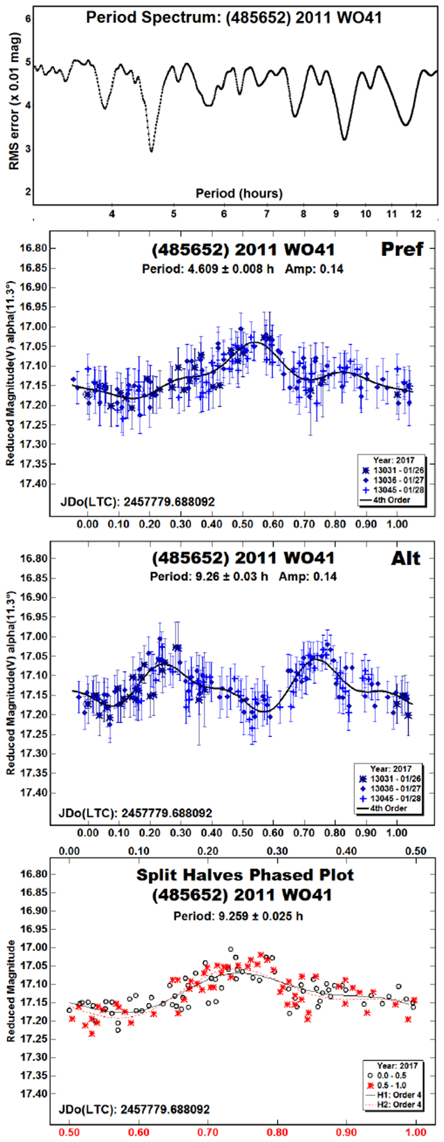
The low amplitude and relatively low phase angle meant that a bimodal lightcurve could not be assumed without supporting evidence. In this case, that evidence was lightcurve that was too symmetrical when the data were forced to a period of about 9.26 hours, i.e., the two halves were so alike as to imply a body that had identically-shaped east/west hemispheres.

A check the help resolve the ambiguity is to plot the data assuming the full period but to overlay the first half of the lightcurve with second half, as shown in the Split Halves plot. If the two halves are essentially identical then, combined with the other information, the half-period with its monomodal shape is the more likely, but not necessarily correct, solution.

2006 EC1, 2013 GL8, 2013 YK148, 2014 AD17, 2015 BN509, and 2016 PR8.

These appear to be the first reported periods for the six NEAs. The solutions for 2013 GL8 and 2013 YK148 are the best estimates based on the obviously noisy data. Of the two, the 64.6 h for 2013 GL8 is the more secure: the lightcurve shape is reasonable and there is multiple coverage of at least one section.

Given the diameter and long period, 2013 GL8 is a good candidate for tumbling (Pravec et al., 2005; 2010). The slopes of the data match the slopes of the Fourier curve; not doing so would be evidence of tumbling. The only thing suspect is the significantly different amplitudes of the two halves. With the amplitude of about 0.65 mag, a more symmetrical lightcurve is usually expected. However, the relatively large phase angle of 37° may have led to shadowing effects that, combined with surface features, produced the asymmetrical shape.

2017 EK.

This is a case of being defeated by all five of the “Fatal Fs”: Faint, Fast (sky motion), Fast rotator, Fading, and Full Moon. At the time of the observations in 2017 mid-March, the asteroid was moving at about 80 arcsec/minute and the almost full moon was less than 50° away. Exposures were kept to 10 seconds. Usually, this is short enough to cover the cases of fast rotator; that was not so in this case.

Pravec et al. (2000) showed that exposures must be kept to

$$E<0.187P$$

where P is the rotation period and E is the exposure in the same units as P. If the exposures are longer than the above would allow, rotation information is “smeared.” As the exposure increases over the limit, it becomes more difficult and, eventually, impossible to find the period.

The issue of exposure time aside, the lightcurve based on the PDS data is almost of no value given the low amplitude in relation to the error bars and random scatter. This was the least of problems. Radar observations (Patrick Taylor, private communications) showed that the rotation period was on the order of 30 seconds. The 10-second exposures were ~0.33P, or almost double the limit given by Pravec et al.

The result given here is almost certainly wrong. This case is being presented as precautionary tale about the many considerations involved in asteroid lightcurve photometry.

2017 AC5, 2017 AF5, 2017 CR32, 2017 DT37, and 2017 BM123.

These appear to be the first reported periods for the five NEAs.

Spin Axis and Shape Models

To model the shape and spin axis of an asteroid usually requires data from multiple apparitions at different phase angle bisector longitudes (viewing aspect). The inversion code uses the information about the changes in the lightcurve versus the viewing aspect to construct a 3-D model that reproduces the original lightcurves as closely as possible.

A wide range of data, over many years is best, allows finding a more accurate sidereal rotation period, which is the foundation upon which all subsequent modeling is done. If the period is wrong, then the model will likely be not just a little, but significantly wrong.

Following the 2017 observations, there were sufficient data to attempt finding a spin axis and shape model for four of the NEAs discussed earlier. They are listed in Table III, which gives the number of dense lightcurves, e.g., those used in this paper, and the number of data sparse points from the Catalina Sky Survey. Table IV gives observing circumstances for each data set for each asteroid. Table V gives the final results. One asteroid, 4055 Magellan, did not have a single, unambiguous solution. The first pole solution is the one that had the lowest χ² value.

Table III.

N_dense is the number of dense lightcurves used in the modeling. The sparse data are considered a single lightcurve, so the N_sparse column gives the number of sparse data points.

Asteroid	Ndense	Nsparse
3103	19	177
4055	21	139
40267	16	189
90075	14	95

Table IV.

Observing circumstances and synodic period results. Pts is the number of data points used in the analysis. The phase angle (α) is given for the first and last date (0h UT); a third, middle value indicates the asteroid reached a minimum during the period. L_PAB and B_PAB are, respectively, the phase angle bisector longitudes and latitudes for the first and last date (0h UT). The Src column gives the reference paper where the original data were used. WS = Wisniewski; V = Velichko; RS = Stephens; AW = Wasczack; W = Warner.

Number	Name	Dates	Pts	Phase	LPAB	BPAB	Period	P.E.	Amp	A.E.	Src
3103	Eger	1987 01/26-02/02	77	20.5,13.8	145	5	5.709	0.001	0.72	0.02	WS91
3103	Eger	1991 07/07-07/17	33	41.9,42.1	318	13	5.707	0.001	0.8	0.1	V92
3103	Eger	2007 02/10-02/17	201	9.4,11.5	143	10	5.711	0.001	0.58	0.02	RS07
3103	Eger	2014 04/20-04/23	167	20.3,20.5	210	31	5.714	0.002	0.45	0.02	W14b
3103	Eger	2016 05/31-06/04	158	43.5,43.9	297	20	5.711	0.002	0.72	0.02	W16b
3103	Eger	2017 02/15-02/16	396	11.1,11.3	147	12	5.710	0.002	0.59	0.02	this
4055	Magellan	2014 01/26-02/01	74	13.4,14.5	113	−23	6.384	0.005	0.76	0.02	W14a
4055	Magellan	2015 04/12-04/17	108	38.7,39.2	255	31	7.496	0.005	0.62	0.04	W15e
4055	Magellan	2017 03/07-03/09	133	1.3,1.0	168	2	7.52	0.01	0.38	0.03	this
40267	1999 GJ4	2013 03/17-04/22	21	15.0,14.9,22.2	181	29	4.958	0.004	0.67	0.03	AW15
40267	1999 GJ4	2014 01/18-01/23	152	34.8,31.4	168	3	4.959	0.002	0.94	0.03	W14a
40267	1999 GJ4	2014 02/24-02/26	237	7.3,6.9	159	10	4.956	0.002	0.86	0.02	W14a
40267	1999 GJ4	2017 02/05-02/08	245	21.6,16.4	157	−1	4.9582	0.0005	1.00	0.03	this
90075	2002 VU94	2014 08/05-08/16	207	42,5,37.5	15	10	7.88	0.01	0.62	0.03	W15a
90075	2002 VU94	2014 10/13-10/14	151	4.1,4.2	18	6	7.90	0.01	0.31	0.02	W15c
90075	2002 VU94	2017 03/30-04/05	216	36.3,42.6	160	−15	7.878	0.002	0.55	0.02	this

Table V.

Pole solutions. L = ecliptic longitude; B = ecliptic latitude; P = sidereal period. The longitude and latitude errors are on the order of ±10°. The period error is approximately 2 units of the last decimal place. The a/b column gives the ratio of the two longest axes (X/Y) of the model. The a/c column gives the ratio of the longest axis (X or Y) versus the Z-axis.

Number	Name	L1	B1	P1	a/b	a/c	L2	B2	P2	a/b	a/c
3103	Eger	211	−76	5.710138	0.75	1.03
4055	Magellan	81	33	7.477559	1.08	1.38	146	87	7.477580	1.20	1.11
40267	1999 GJ4	63	37	4.957067	1.46	2.28
90075	2002 VU94	73	−50	7.878512	1.25	1.76

MPO LCInvert was used for the inversion work. This is a Windows-based wrapper around the original C/FORTRAN code developed first by Kaasalainen et al. (2001a; 2001b). The reader is referred to the paper by Warner et al. (2017b) elsewhere in this issue for details about the inversion process and approach taken to derive the spin axis and shape models. That paper also discusses certain features of derived models, specifically flat zones on the model and their physical interpretation.

The results of the modeling are presented at the end of this paper. There are several plots for each asteroid that were generated by MPO LCInvert. For each group of plots, the left-hand plot on the first line shows the L_PAB distribution. Green circles represent the mid-point of each dense lightcurve. Red squares represent each sparse data point. The right-hand plot of the first line shows the period search χ² values versus period. The horizontal green line is at 1.1x the lowest χ² value, i.e., the so-called “10% rule” discussed in Warner et al. (2017b).

On the second line, the left-hand image is the 10% pole search plot. Each small region represents a 15x15° area of the sky in ecliptic coordinates. Deep blue represents the area with the lowest χ². The colors move towards bright red, which represents the 10% cutoff. Anything more than 10% is dark red. The perfect solution is a single deep blue island in a sea of dark red. The additional image(s) on the second line show profiles of the asteroid model as viewed from over the north and south poles and in the asteroid’s equatorial plane at Z = 0° and Z = +90° rotation.

Since the inversion algorithms used here find only a convex hull, concavities appear as large flat areas on the asteroid. A good analogy is to imagine wrapping the asteroid with paper without punching holes in the paper to fill depressions. This creates flat areas in the wrapping that are covering concavities.

The remaining plots compare the dense data with the model curve at specific times. The red dots represent the dense data while the solid black line is the model lightcurve. The main test is if the dense lightcurve has the same amplitude and shape as the model lightcurve. If there are multiple pole solutions, then the one that gives the best fits for all the dense lightcurves is the more likely solution – assuming it has a realistic shape. If the rotation rate is being affected by YORP, then the model lightcurves will slowly become out of phase with the data, e.g., maximums not quite aligning in rotation phase.

Figure 1:

3103 Eger. The pole solution is unambiguous with regards to the negative latitude, which indicates a retrograde rotation. The fit of the models to the data is surprisingly good since Durech et al. (2012) established that the sidereal rotation period is slowly increasing over time. See the text for an explanation of the plots.

Figure 2:

4055 Magellan. The favored pole is (81°, 33°). The alternate solution, with an obliquity of nearly 0°, cannot be formally excluded. When the latitude is very near one of the ecliptic poles, the uncertainty in the longitude is significantly higher. The poor fit of the models lightcurves to the actual data, especially in 2014 January, reflect the uncertainty of both the period and pole solution. See the text for an explanation of the plots.

Figure 3:

(40267) 1999 GJ4. Dense data were available from only two apparitions. The data set from Waszczak et al. (2015) had fewer than 25 data points spread over several weeks. They were treated as dense data since they were all from the same apparition. Regardless of their status, the data confined the pole solution to a smaller area than when not being used. The larger amplitude of the actual data and the large flat areas in the model may indicate that this is a highly bifurcated body. See the text for an explanation of the plots.

Figure 4:

(90075) 2002 VU94. Only one pole solution is given here despite the apparent second solution that differs by about 180° in longitude. The colors of the regions at the second solution mostly indicate that it was just within the 10° rule. Additional observations may eventually prove that second solution to be the correct one. The model fits to the data are very good. See the text for an explanation of the plots.

Table II.

Observing circumstances. Pts is the number of data points used in the analysis. The phase angle (α) is given at the start and end of each date range, unless it reached a minimum, which is then the second of three values. If a single value is given, the phase angle did not change significantly and the average value is given. L_PAB and B_PAB are, respectively the average phase angle bisector longitude and latitude, unless two values are given (first/last date in range). Grp is the orbital group of the asteroid. See Warner et al. (LCDB; 2009; Icarus 202, 134-146.).

Number	Name	2016 mm/dd	Pts	Phase	LPAB	BPAB	Period	P.E.	Amp	A.E.	Grp
2102	Tantalus	01/06-01/18	297	75.0,81.1	62	28	2.383	0.001	0.07	0.01	NEA
2329	Orthos	02/25-03/03	109	18.6,17.1	195	10	6.178	0.005	0.67	0.05	NEA
3103	Eger	02/15-02/16	396	11.2,11.4	147	12	5.710	0.002	0.60	0.02	NEA
4055	Magellan	03/07-03/09	133	1.2,1.0,1.2	168	2	7.52	0.01	0.38	0.03	NEA
5604	1992 FE	03/23-03/26	122	38.5,39.3	160	−12	5.337	0.004	0.21	0.02	NEA
5626	1991 FE	01/30-03/02	407	21.0,6.9	175	0	133.5	0.4	0.13	0.02	NEA
5693	1993 EA	01/27-01/29	605	6.7,7.6	126	6	2.496	0.002	0.05	0.01	NEA
10636	1998 QK56	03/17-03/19	442	29.2,28.9	157	−2	9.876	0.004	0.53	0.03	NEA
11398	1998 YP11	01/29-02/24	417	12.6,5.4,16.7	141	−2	38.59	0.01	0.20	0.02	NEA
22771	1999 CU3	02/23-03/02	123	24.6,21.8	181	−4	3.781	0.002	0.23	0.02	NEA
40267	1999 GJ4	02/05-02/08	245	21.6,16.4	157	−1	4.9582	0.0005	1.00	0.03	NEA
90075	2002 VU94	03/30-04/05	216	36.3,42.6	160	−15	7.878	0.002	0.55	0.02	NEA
137158	1999 FB	03/28-03/29	130	11.2,10.7	191	11	6.074	0.005	1.18	0.03	NEA
138155	2000 ES70	03/28-04/02	130	18.8,21.8	168	0	5.131	0.002	0.16	0.02	NEA
138359	2000 GX127	03/30-04/03	155	25.0,21.7	204	19	3.685	0.003	0.06	0.01	NEA
143404	2003 BD44	02/25-03/17	409	18.1,3.3	177	−1	29.71	0.01	0.42	0.02	NEA
153951	2002 AC3	01/30-02/01	235	21.8,20.9	148	−2	7.072	0.002	1.09	0.03	NEA
203471	2002 AU4	01/16-01/18	428	27.9,28.2	122	19	13.26	0.02	1.32	0.04	NEA
252091	2000 UP30	03/30-04/03	111	1.7,5.2	188	−1	5.44	0.01	0.22	0.02	NEA
370307	2002 RH52	03/07-03/09	183	24.2,21.9	188	3	4.219	0.002	0.36	0.03	NEA
405427	2004 ST9	04/04-04/06	91	11.8,13.4	182	−3	5.203	0.003	0.74	0.05	NEA
483508	2003 CR1	01/27-02/05	680	52.5,32.7	159	−5	26.32	0.03	1.35	0.10	NEA
484795	2009 DE47	03/24-03/29	182	43.2,35.1	205	21	5.997	0.005	0.24	0.02	NEA
485652	2011 WO41	01/26-01/28	130	11.3,11.0	135	12	4.609	0.008	0.14	0.02	NEA
	2006 EC1	02/23-02/24	231	53.5,50.9	171	34	5.15	0.02	0.25	0.03	NEA
	2013 GL8	01/28-02/16	1027	36.5,1.9	154	3	64.6	0.5	0.68	0.05	NEA
	2013 YK148	02/25-03/03	456	45.0,31.9	158	29	16.3	0.1	0.30	0.03	NEA
	2014 AD17	01/16-01/18	135	4.3,5.1	118	−3	8.48	0.02	0.22	0.03	NEA
	2015 BN509	01/26-01/27	169	37.5,38.2	151	4	5.683	0.004	1.01	0.03	NEA
	2016 PR8	12/29-01/18	123	51.3,27.6	134	15	16.17	0.01	0.39	0.04	NEA
	2017 EK	03/14-03/14	228	57.8,57.8	194	22	0.297	0.002	0.30	0.05	NEA
	2017 AC5	03/18-03/27	243	6.5,14.6	176	4	5.922	0.005	0.81	0.03	NEA
	2017 AF5	01/16-01/29	892	24.4,8.5	132	11	49.68	0.06	0.35	0.04	NEA
	2017 CR32	03/18-03/27	506	15.6,0.2,8.0	183	2	14.91	0.02	0.41	0.03	NEA
	2017 DT37	03/27-04/02	199	17.8,13.8	203	6	14.605	0.006	0.55	0.03	NEA
	2017 BM123	02/23-02/24	921	26.8,31.9	168	9	2.15	0.005	0.37	0.05	NEA

References

- Bembrick C, Pereghy B (2003). “A period determination for the Aten asteroid (5604) 1992 FE.” Minor Planet Bull. 30, 43–44. [Google Scholar]
- Durech J, Vokrouhlicky D, Baransky AR, Breiter S, Burkhonov OA, Cooney W, Fuller V, Faftonyuk NM, Gross J, Inasaridze R Ya., and 21 coauthors. (2012). “Analysis of the rotation period of asteroids (1865) Cerberus, (2100) Ra-Shalom, and (3103) Eger - search for the YORP effect.” Astron. Astrophys. 547, A10. [Google Scholar]
- Harris AW, Young JW, Scaltriti F, Zappala V (1984). “Lightcurves and phase relations of the asteroids 82 Alkmene and 444 Gyptis.” Icarus 57, 251–258. [Google Scholar]
- Harris AW, Young JW, Bowell E, Martin LJ, Millis RL, Poutanen M, Scaltriti F, Zappala V, Schober HJ, Debehogne H, Zeigler KW (1989). “Photoelectric Observations of Asteroids 3, 24, 60, 261, and 863.” Icarus 77, 171–186. [Google Scholar]
- Harris AW, Pravec P, Galad A, Skiff BA, Warner BD, Vilagi J, Gajdos S, Carbognani A, Hornoch K, Kusnirak P, Cooney WR, Gross J, Terrell D, Higgins D, Bowell E, Koehn BW (2014). “On the maximum amplitude of harmonics on an asteroid lightcurve.” Icarus 235, 55–59. [Google Scholar]
- Henden AA, Terrell D, Levine SE, Templeton M, Smith TC, Welch DL (2009). http://www.aavso.org/apass
- Higgins D, Warner BD (2009). “Lightcurve Analysis at Hunters Hill Observatory and Collaborating Stations - Autumn 2009.” Minor Planet Bull. 36, 159–160. [Google Scholar]
- Kaasalainen M, Torppa J (2001a). “Optimization Methods for Asteriod Lightcurve Inversion. I. Shape Determination.” Icarus 153, 24–36. [Google Scholar]
- Kaasalainen M, Torppa J, Muinonen K (2001b). “Optimization Methods for Asteriod Lightcurve Inversion. II. The Complete Inverse Problem.” Icarus 153, 37–51. [Google Scholar]
- Koehn BW, Bowell ELG, Skiff BA, Sanborn JJ, McLelland KP, Pravec P, Warner BD (2014). “Lowell Observatory Near-Earth Asteroid Photometric Survey (NEAPS) - 2009 January through 2009 June.” Minor Planet Bul. 41, 286–300. [Google Scholar]
- Krugly Yu.N., Bel’skaya IN, Shevchenko VG, Chorny VG, Velichko FP, Mottola S, Erikson A, Hahn G, Nathues A, Neukum G, Gaftonyuk NM, Dotto E (2002). “The Near-Earth Objects Follow-up Program. IV. CCD Photometry in 1996-1999.” Icarus 158, 294–304. [Google Scholar]
- Polishook D (2012). “Spectral and spin measurement of two small and fast-rotating near-Earth asteroids.” Minor Planet Bull. 39, 187–192. [Google Scholar]
- Pravec P, Wolf M, Sarounova L (2000 web, 2003 web). http://www.asu.cas.cz/~ppravec/neo.htm [Google Scholar]
- Pravec P, Hergenrother C, Whiteley R, Sarounova L, Kusnirak P (2000). “Fast Rotating Asteroids 1999 TY2, 1999 SF10, and 1998 WB2.” Icarus 147, 477–486. [Google Scholar]
- Pravec P, Harris AW, Scheirich P, Kušnirák P, Šarounová L, Hergenrother CW, Mottola S, Hicks MD, Masi G, Krugly Yu.N., Shevchenko VG, Nolan MC, Howell ES, Kaasalainen M, Galád A, Brown P, Degraff DR, Lambert JV, Cooney WR, Foglia S (2005). “Tumbling asteroids.” Icarus 173, 108–131. [Google Scholar]
- Pravec P, Scheirich P, Durech J, Pollock J, Kusnirak P, Hornoch K, Galad A, Vokrouhlicky D, Harris AW, Jehin E, Manfroid J, Opitom C, Gillon M, Colas F, Oey J, Vrastil J, Reichart D, Ivarsen K, Haislip J, LaCluyze A (2014). “The tumbling state of (99942) Apophis.” Icarus 233, 48–60. [Google Scholar]
- Rubincam DP (2000). “Relative Spin-up and Spin-down of Small Asteroids.” Icarus 148, 2–11. [Google Scholar]
- Stephens RD (2007). Data from ALCDEF database. http://www.alcdef.org
- Velichko FP, Krugly Yu.N., Chiornij VG (1992). <Title not available>. Astron. Tsirk 1553, 37–38. [Google Scholar]
- Warner BD (2007). “Initial Results of a Dedicated H-G Program.” Minor Planet Bull. 34, 113–119. [Google Scholar]
- Warner BD (2008). “Asteroid Lightcurve Analysis at the Palmer Divide Observatory: February-May 2008.” Minor Planet Bull. 35, 163–167. [PMC free article] [PubMed] [Google Scholar]
- Warner BD, Harris AW, Pravec P (2009). “The Asteroid Lightcurve Database.” Icarus 202, 134–146. Updated 2017 April. http://www.minorplanet.info/lightcurvedatabase.html [Google Scholar]
- Warner BD (2014a). “Near-Earth Asteroid Lightcurve Analysis at CS3-Palmer Divide Station: 2014 January-March.” Minor Planet Bull. 41, 157–168. [PMC free article] [PubMed] [Google Scholar]
- Warner Brian D. (2014b). “Near-Earth Asteroid Lightcurve Analysis at CS3-Palmer Divide Station: 2014 March-June.” Minor Planet Bull. 41, 213–224. [PMC free article] [PubMed] [Google Scholar]
- Warner BD (2015a). “Near-Earth Asteroid Lightcurve Analysis at CS3-Palmer Divide Station: 2014 June-October.” Minor Planet Bull. 42, 41–53. [PMC free article] [PubMed] [Google Scholar]
- Warner BD (2015b). “A Quartet of Near-Earth Asteroid Binary Candidates.” Minor Planet Bull. 42, 79–83. [PMC free article] [PubMed] [Google Scholar]
- Warner BD (2015c). “Near-Earth Asteroid Lightcurve Analysis at CS3-Palmer Divide Station: 2014 October-December.” Minor Planet Bull. 42, 115–127. [PMC free article] [PubMed] [Google Scholar]
- Warner BD (2015d). “Near-Earth Asteroid Lightcurve Analysis at CS3-Palmer Divide Station: 2015 January – March.” Minor Planet Bull. 42, 172–183. [PMC free article] [PubMed] [Google Scholar]
- Warner BD (2015e). “Near-Earth Asteroid Lightcurve Analysis at CS3-Palmer Divide Station: 2015 March-June.” Minor Planet Bull. 42, 256–266. [PMC free article] [PubMed] [Google Scholar]
- Warner BD (2016a). “Three Additional Candidates for the Group of Very Wide Binaries.” Minor Planet Bul. 43, 306–309. [PMC free article] [PubMed] [Google Scholar]
- Warner BD (2016b). “Near-Earth Asteroid Lightcurve Analysis at CS3-Palmer Divide Station: 2016 April-July.” Minor Planet Bull. 43, 311–319. [PMC free article] [PubMed] [Google Scholar]
- Warner BD (2017a). “Near-Earth Asteroid Lightcurve Analysis at CS3-Palmer Divide Station: 2016 July-September.” Minor Planet Bul. 44, 22–36. [PMC free article] [PubMed] [Google Scholar]
- Warner BD, Pravec P, Kusnirak P, Benishek V, Ferrero A (2017b). “Preliminary Pole and Shape Models for Three Near-Earth Asteroids.” Minor Planet Bul. 44, 206–212. [PMC free article] [PubMed] [Google Scholar]
- Waszczak A, Chang C-K, Ofek EO, Laher R, Masci F, Levitan D, Surace J, Cheng Y-C, Ip W-H, Kinoshita D, Helou G, Prince TA, Kulkarni S (2015). “Asteroid Light Curves from the Palomar Transient Factory Survey: Rotation Periods and Phase Functions from Sparse Photometry.” Astron. J 150, A75. [Google Scholar]
- Wisniewski WZ (1991). “Physical studies of small asteroids. I - Lightcurves and taxonomy of 10 asteroids.” Icarus 90, 117–122. [Google Scholar]
- Zappala V, Cellini A, Barucci AM, Fulchignoni M, Lupishko DE (1990). “An analysis of the amplitude-phase relationship among asteroids.” Astron. Astrophys 231, 548–560. [Google Scholar]