19204 JOSHUATREE – NOT SO FAST

Abstract

CCD photometric observations in 2016 February and March and a reevaluation of observations made in 2013 June of 19204 Joshuatree show it to be a possible binary. It is another candidate for the special case of very wide binaries. The primary lightcurve has a period of 480 ± 5 h and an amplitude 0.25 ± 0.02 mag. and the secondary lightcurve has a period of 21.25 ± 0.05 h.

19204 Joshuatree was discovered by Jean E. Mueller in 1992 as part of the POSS II survey at Palomar Observatory. She recently named the asteroid after Joshua Tree National Park, near where she now lives. She contacted us in hopes of obtaining a rotational period to augment a presentation to park officials featuring the naming of the asteroid. Since we doubt the Superintendent of Joshua Tree National Park or the Yucca Valley City Council are regular readers of the Minor Planet Bulletin, we feel safe in announcing the results here.

We informed Mueller that a previous lightcurve had been obtained by the authors in 2006 and 2013 (Stephens, 2006; Warner, 2013). The most definitive result was a 19.55 h period obtained by Warner from observations in 2013 June obtained at the Center for Solar System Studies (CS3, MPC U81), also near Joshua Tree National Park. However, this lightcurve had a low amplitude, a single extrema, and did not have dense coverage over the range of the lightcurve due to the short summer nights in the Northern Hemisphere. With an amplitude of only 0.08 mag., it is possible that the lightcurve could have only a single extrema, or three or more extrema (Harris et al, 2014). Because of this, the 2013 result had a U = 2 rating in the asteroid lightcurve database (LCDB; Warner et al., 2009), meaning that the period may be wrong by 30 percent or more. To assist Mueller in her presentation and remove the ambiguity, we agreed to reobserve Joshuatree in 2016.

Observations

The observations were made by Stephens using a 0.35-m Schmidt-Cassegrain telescope with Finger Lakes MicroLine ML-1001E CCD camera. The 300-second exposures were unguided and made without a filter. Table I gives the observation circumstances over a span of over a month.

Table I.

Observing circumstances for 19204 Joshuatree during the 2016 observing apparition. The last two columns are the phase angle bisector longitude and latitude (see Harris et al., 1984). The values were computed for 8 h UT, or about the middle of each observing run.

2016 mmm/dd	Phase	LPAB	BPAB
Feb 26	10.83	142.7	15.2
Feb 28	11.64	142.7	15.4
Mar 01	12.45	142.7	15.6
Mar 02	12.87	142.7	15.7
Mar 07	14.93	142.7	16.3
Mar 09	15.74	142.7	16.5
Mar 10	16.13	142.7	16.5
Mar 13	17.30	142.8	16.8
Mar 15	18.06	142.9	17.0
Mar 16	18.43	143.0	17.1
Mar 17	18.79	143.0	17.2
Mar 18	19.14	143.1	17.3
Mar 24	21.14	143.5	17.7
Mar 25	21.45	143.6	17.8
Mar 26	21.75	143.7	17.9
Mar 27	22.05	143.8	17.9
Mar 28	22.34	143.9	18.0

The raw images were flat-field and dark subtracted before being measured in MPO Canopus. Night-to-night linkage was aided by the Comp Star Selector utility which helps find near-solar color comparison stars, thus reducing color difference issues. Stars were chosen from the MPOSC catalog, which is based on the 2MASS catalog (http://irsa.ipac.caltech.edu/Missions/2mass.html). The J-K magnitudes in 2MASS were converted to V magnitudes using formulae by Warner (2007). Generally, needed zero points adjustments are within ±0.05 of one another, but larger adjustments can be required to minimize the RMS value from the Fourier analysis.

Period Analysis

Period analysis was done using MPO Canopus, which employs the FALC Fourier analysis algorithm developed by Harris (Harris et al., 1989). MPO Canopus can do a dual-period search process. The program first finds an initial value for the dominant (usually shorter) period. The Fourier model lightcurve is subtracted from the data set in the succeeding search for a second period. The Fourier curve for that second period is then subtracted from the data set in a new search for the dominant period. The iterative process continues until both periods stabilize and it produces reasonable lightcurves.

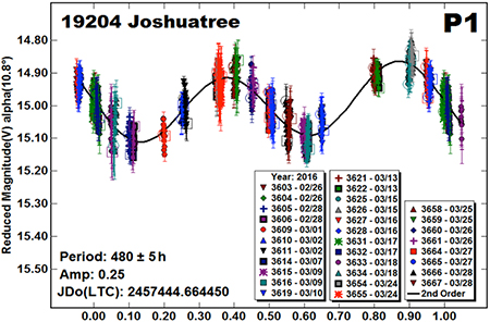
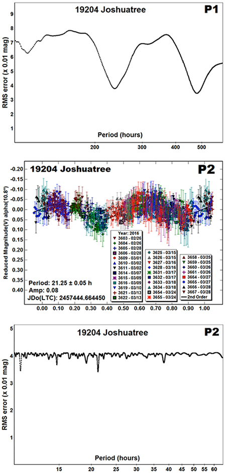
The dual period analysis found a primary lightcurve of P₁ = 480 ± 5 h, A₁ = 0.25 ± 0.02 mag (“P1” plot). Assuming an equatorial view of the asteroid, this leads to an a/b ratio of the asteroid’s silhouette of 1.26:1. As expected, subtracting this lightcurve from the data set and doing a period search found a solution that showed no mutual events (occultations and/or eclipses) due to a satellite (“P2” plot). The lightcurve has a period of P₂ = 21.25 ± 0.05 h, A₂ = 0.08 mag. The lightcurve was essentially flat, which likely indicates a nearly spheroidal shape for the satellite.

With the finding of a long period component of the lightcurve, Warner reevaluated the 2013 data. By removing all nightly zero point adjustments, Warner was able to show a large amplitude in the dataset over the five night span, consistent with a 480 h primary period. The phase angle bisector longitude for the 2013 observations was 263°, significantly different from the 2016 observations. There were insufficient data to solve for a secondary period.

Stephens’ 2006 observations were made before the creation of the MPOSC catalog, so he remeasured the original images which were still available a decade later. The phase angle bisector longitude during the 2006 observations was 253°, similar to those from the 2013 observations. However, the observations occurred on four nights with a two week gap in between; sufficient to mask any large changes in amplitude. Plotting for the possible secondary period of 21.25 h is consistent a single modal lightcurve with coverage of about 60% of the lightcurve.

Analysis

19204 Joshuatree is another possible candidate for a special case of very wide binaries (see Jacobson et al, 2014). This is where the primary period is long with a large amplitude and the secondary period is short with a low amplitude. For wide binaries, the chance of observing a mutual event (eclipse or occultation) would be very rare because of the long primary period. Table II gives a list of suspected wide binary asteroids. Because of the lack of mutual events, confirmation of the nature of these asteroids will require long observing runs at future oppositions.

Table II.

List of suspected wide binary asteroids. P1 is the primary’s period (hours). P2 is the satellite’s, which is not tidally-locked to its orbital period. All references are Warner (et al.).

Number	Name	P1	P2	Ref
1876	Napolitania	45	2.825	MPB 43, 57–65
8026	Johnmckay	372	2.2981	MPB 38, 33–36
15778	1993 NH	113	3.320	MPB 42, 60–66
19204	Joshuatree	480	21.25	This work
23615	1996 FK12	368	3.6456	MPB 42, 182–186
67175	2000 BA19	275	2.7157	MPB 42, 36–42
119744	2001 YN42	624	7.24	MPB 41, 102–112
190208	2006 AQ	182	2.621	MPB 42, 79–83
218144	2002 RL66	588	2.49	MPB 37, 109–111
	2014 PL51	205	5.384	MPB 42, 134–136

The long period (P1) might suggest tumbling. This was rejected because of the short period and its amplitude. The two periods for a true tumbler should be within a factor of two of one another when one of the amplitudes is so large. Additional insights into this reasoning were provided by Alan Harris (private communications).

“A large amplitude indicates a very irregular (elongate) object, so the two tumble frequencies should be not far apart since the ‘precession’ frequency is essentially the moment of inertia differences (elongation or flattening of the object) times the ‘rotation’ frequency. For a very regularly shaped body (hence very low lightcurve amplitude), the precession frequency can be much longer than the rotation frequency, for example, for the Earth, the ‘Chandler wobble’ period is around 300 days. The bottom line, though, is that the long period of this one is unlikely (impossibly, in fact) due to tumbling of a single body.”

Conclusion

There are a couple of lessons to be learned. The first is when using a star catalog of standard or secondary standard stars is to trust the data and follow through when needed. A second point concerns the wide spread practice of only getting a few data points each night when a long period asteroid is found. While understandable when telescope observing time is limited to a few days, one has to wonder how many binary or otherwise unusual asteroids went undiscovered because it was assumed that a long period asteroid will not have a satellite. In these ten cases, the satellites would not have been discovered without truly dense lightcurve data.

References

- Harris AW, Young JW, Scaltriti F, Zappala V (1984). “Lightcurves and phase relations of the asteroids 82 Alkmene and 444 Gyptis.” Icarus 57, 251–258. [Google Scholar]
- Harris AW, Young JW, Bowell E, Martin LJ, Millis RL, Poutanen M, Scaltriti F, Zappala V, Schober HJ, Debehogne H, Zeigler KW (1989). “Photoelectric Observations of Asteroids 3, 24, 60, 261, and 863.” Icarus 77, 171–186. [Google Scholar]
- Harris AW, Pravec P, Galád B Skiff B, Warner B, Világi J, Gajdoš S, Carbognani A, Hornoch K, Kušnirák P, Cooney W, Gross J, Terrell D, Higgins D, Bowell E, Koehn B. (2014) “On the maximum amplitude of harmonics of an asteroid lightcurve.” Icarus 235, 55–59. [Google Scholar]
- Jacobson SA, Scheeres DJ, McMahon J (2014). “Formation of the Wide Asynchronous Binary Asteroid Population.” Ap. J. 780:60. [Google Scholar]
- Stephens RD. (2006). “Asteroid lightcurve photometry from Santana and GMARS observatories - winter and spring 2006.” Minor Planet Bull. 33, 100–101. [Google Scholar]
- Warner BD (2013). “Asteroid Lightcurve Analysis at CS3-Palmer Divide Station: 2013 May-June.” Minor Planet Bul. 40, 208–212. [PMC free article] [PubMed] [Google Scholar]
- Warner BD (2007). “Initial Results of a Dedicated H-G Program.” Minor Planet Bul. 34, 113–119. [Google Scholar]
- Warner BD, Harris AW, Pravec P (2009). “The Asteroid Lightcurve Database.” Icarus 202, 134–146. Updated 2016 Feb. http://www.minorplanet.info/lightcurvedatabase.html [Google Scholar]