EpithNet: Deep Regression for Epithelium Segmentation in Cervical Histology Images

Abstract

Background:

Automated pathology techniques for detecting cervical cancer at the premalignant stage have advantages for women in areas with limited medical resources.

Methods:

This article presents EpithNet, a deep learning approach for the critical step of automated epithelium segmentation in digitized cervical histology images. EpithNet employs three regression networks of varying dimensions of image input blocks (patches) surrounding a given pixel, with all blocks at a fixed resolution, using varying network depth.

Results:

The proposed model was evaluated on 311 digitized histology epithelial images and the results indicate that the technique maximizes region-based information to improve pixel-wise probability estimates. EpithNet-mc model, formed by intermediate concatenation of the convolutional layers of the three models, was observed to achieve 94% Jaccard index (intersection over union) which is 26.4% higher than the benchmark model.

Conclusions:

EpithNet yields better epithelial segmentation results than state-of-the-art benchmark methods.

INTRODUCTION

In recent years, the number of cervical cancer cases worldwide has increased, making it the fourth most frequent cancer in women. It is estimated that a total of 570,000 new cases were reported in 2018, 6.6% of all female cancers. Low- and middle-income countries account for 90% of deaths from cervical cancer.[1] The prevention of cervical cancer mortality is possible with earlier treatment through screening and earlier diagnosis at the precancer stage. The standard diagnostic process is the microscopic evaluation of histology images by a qualified pathologist.[2,3] The severity of cervical precancer typically increases as the immature atypical cells increase across the epithelium region. Based on this observation, the precancer condition affecting squamous epithelium is classified as normal or three grades of cervical intraepithelial neoplasia (CIN): CIN1, CIN2, and CIN3.[4,5,6] Normal means there is no dysplasia and CIN1, CIN2, and CIN3 correspond to mild, moderate, and severe dysplasia, respectively. As the severity of the dysplasia increases, an increase in the density of immature atypical cells can be observed from the lamina propria (region below the epithelium) to the outer layer of the epithelium. Figure 1 shows the cervical histology digital microscopy (DM) image at ×10 containing background, stratified squamous epithelium, and lamina propria, with the epithelial binary mask (right) determined manually by a pathologist.

Figure 1.

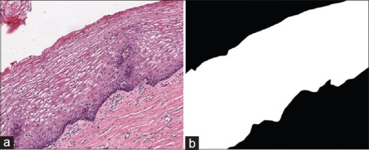
(a) Digital microscopy image at ×10 magnification with corresponding (b) manually generated mask

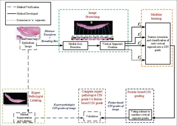
Pathologists examine the epithelial regions of the cervical histology slides under a light microscope after a biopsy. The regions of lamina propria and background, which occupy the majority of the image area, are not the regions of interest during the analysis. The whole-slide DM image is usually an ultra-large image, up to 40 K × 80 K pixels. This makes the manual examination of the DM image and segmentation of the epithelium region a tedious job. As a future step toward segmenting the epithelium in the whole-slide image, we work with the high-resolution subimages containing epithelium that share the borders with lamina propria and background, as depicted in Figure 1a. These subimages have been cropped from the whole-slide image by the pathologist. Figure 2 shows the epithelium analysis process that has been explored in previous research[7,8] using manual epithelium region segmentation. The segmented epithelium regions were split into multiple vertical segments with reference to the detected medial axis. Each vertical segment is processed to extract a set of 27 features which are later categorized into a CIN grade by applying traditional machine learning algorithms. All the predicted CIN grades were fused through a voting scheme to generate a single CIN grade representing the entire image. The fusion-based CIN grades were evaluated against the labels provided by the expert pathologist.

Figure 2.

Epithelium analysis process used in previous research based on a manually segmented epithelium

The goal of this research is to automate the epithelium analysis process. The primary step that needs automation is segmentation of epithelium regions to facilitate computer-assisted feature and CIN classification to assist the pathologist in the diagnostic process.

In this article, we propose an automated segmentation of epithelium regions at high resolution of ×10 histology images, which can be applied to accurate segmentation of epithelium regions in both high-resolution and low-resolution images.

We explore the possibility of constructing small-scale but efficient convolutional neural networks (CNNs) to solve the difficult automated segmentation task. The task is challenging due to the varying levels of hematoxylin and eosin staining, the varying shapes of epithelial regions, the varying density and shape of cells in these regions, the presence of blood in the tissue sample, and the presence of columnar cellular regions. CNNs extract hierarchal features, which contain information about patterns, colors, textures, etc. These features help the model to better predict a pixel-wise probability of a pixel belonging to the epithelium region. We design a CNN regression model that can analyze the spatial information around a pixel in the form of input image data and learn the features to assign a probability value of being epithelial pixel.

In the last decade, various studies have been published on the epithelium segmentation topic with the help of conventional image processing techniques. A multiresolution segmentation strategy[9] was developed to segment squamous epithelial layer in virtual slides. The segmentation was initially performed on a low-resolution image and later tuned at higher resolution of ×40 by utilizing an iterative boundary expanding-shrinking method. This is a block segmentation approach implemented with a support vector machine classifier using textural features of the image. This work was further extended[5] to diagnose CIN from the changes of density of nuclei along the perpendicular line feature. Feature-based automated segmentation was proposed[10] to segment pan-cytokeratin-stained histology images of lung carcinoma by extracting superpixels. The results were analyzed using leave-one-out methodology and achieved a Dice coefficient score of 91% for vital tumor and 69% for necrosis. Local binary patterns[11] were analyzed for precise and better segmentation of image samples from video content of respiratory epithelium. U-Net[12] is a popular deep learning (DL) approach for biomedical image segmentation that is successful in segmenting various biomedical images, which we use for benchmark performance comparison in this study, where we investigate creation of an epithelium probability mask through regression analysis using a DL framework.

METHODS

The proposed method of epithelium segmentation is based on the idea of estimating the probability that a given pixel represents epithelium. The rationale for the probabilistic model is that, unlike segmentation of more defined biological samples such as the heart or liver, which have a discrete boundary, microscopic tissue segmentation boundaries marked by pathologists can vary significantly. A neighborhood of n × m pixels centered on the pixel of interest to be passed to a CNN model is shown in Figure 3. The resultant scalar represents the probability that the pixel at the center of the given neighborhood belongs to the epithelium. This continues in sliding-window fashion until each pixel in the digital epithelium image is processed. The final output is a probability map.

Figure 3.

Generation of labels

Data

The dataset for this research consisted of 351 high-resolution DM histology color images and corresponding manually segmented epithelial layer masks, as shown in Figure 1a and b, respectively. The manually generated masks were verified and approved by expert pathologists, including 40 histology images representing the diversity of the data (10 images from each CIN class). The cervical histology images have varying density of nuclei and cytoplasm. There are images with dark and larger nuclei with thick cytoplasm, images with dark and smaller nuclei with moderate cytoplasm, and images with light and relatively moderate size nuclei with light cytoplasm. Furthermore, varying CIN grades show varying nuclear densities in the epithelium regions. These 40 images were employed for training the model, and the remaining 311 images were used for testing and evaluating the performance of the model.

Overview of proposed segmentation method

The proposed epithelial segmentation task is split into four parts: (1) data preprocessing, (2) training, (3) testing, and (4) postprocessing. The data preprocessing is the first step that deals with generation of smaller patch image data and normalizing the data. Section C highlights the details. Training and testing include creating a regression CNN model and usage of memory-optimized workflow in the testing phase. Section D provides more details about the architecture and workflow. Postprocessing includes thresholding and generating a binary mask which is further cleaned and smoothened over the edges. Section E provides insights about the postprocessing steps.

Input image data

CNNs need voluminous image data of a standard shape as input. The limited availability of annotated data in this domain, consisting of 351 images of varying sizes here, is a major challenge. The dissimilar size issue could be rectified by resizing images to a standardized size, but this may introduce problems relating to cropping, aspect ratio, and padding. Even if the dissimilar image sizes were not an issue, the small number of image samples is. The solution to the small dataset and dissimilar image sizes was to decompose each image into a set of overlapping (n, m) patches with a patch stride s. An epithelial image of size (N, M) would generate P patches (Equation 1).

The image data are decomposed using Equation 1, with patch size (n, m) = ([16, 16], [32, 32], [64, 64]) and stride s =16 for training data and s = 4 for test data. This way the original RGB image and the binary ground-truth masks are decomposed into a set of n × m ×3 and n × m ×1, respectively, overlapping patches.

A training image dataset was created by considering 40 images representative of the four CIN grades. These images were chosen such that the network could learn various characteristic features of the histology images with different shapes, colors, and densities of nuclei and cytoplasm in both epithelial and lamina propria regions. A total of 254,514 image patches of size n × m ×3 were generated, with 85% of the data used for the training dataset and the remaining data used to validate the trained model.

A CNN is used to solve the regression problem by predicting the probability of each pixel of the image belonging to the epithelium region. The ground-truth patches were further reduced to a numerical representation of the percentage of non-zero pixels within a given mask patch, as shown in Figure 3. If the non-zero pixels in a mask patch, P_mask, were assigned a value of 1, the average epithelium density, μ, of each patch is given by

The ground-truth probability value for each patch is defined by the μ value.

Regression model

Next, a regression model is determined using a CNN to predict the average epithelium density (used interchangeably with probability) in each patch image. CNNs are mostly used to classify images. The classification task has a discrete output. However, to predict probability on neighboring blocks of images, we consider the neighboring blocks as continuous data that can be handled better through a regression model, and hence, we include a single neural node at the end of the network.

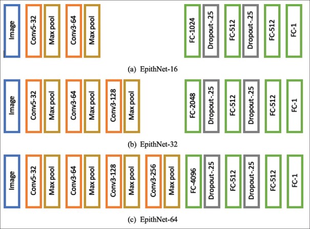
We design CNN models that are variants of a VGG network[13] in terms of filter’s receptive field and depth. These models are fed with block images (RGB) of sizes 16 × 16, 32 × 32, or 64 × 64, as shown in Figure 4. The models are named as EpithNet-16, EpithNet-32, and EpithNet-64, where the postscript represents the size of the input image that the model can read. Each image is subjected to a stack of convolutional layers (Conv), where the first-layer filter has a receptive field of 5 × 5 and the following layers are designed to have 3 × 3 filters. Spatial padding is applied such that the output layer has size same as the input layer after the convolution operation. The stride is fixed to 1. Each convolutional layer is followed by a 2 × 2 max-pooling layer. A series of convolutional and max-pooling layers are stacked with increasing feature depth until a layer of size 4 × 4 is obtained. These are then followed by four fully connected (FC) layers. The first FC layer has 4096 nodes, followed by two FC layers containing 512 nodes, and finally a single node FC layer which is an output regression layer.

Figure 4.

EpithNet architecture

For activation functions, the Conv layers are implemented with ReLU,[14] FC layers with leaky ReLU,[15] and the output layer with tanh. Dropout layers were included to regularize the model to avoid overfitting.

The model is trained with augmented data. The input data are randomly augmented with shear range varying from 0 to 10 and random rotation of images between 0° and 90°. The model is compiled with the Adadelta optimizer,[16] which adapts the learning rate based on gradient updates. The learning rate is set to 1.0, and the gradient decay factor at each time step is set to 0.95. The loss functions investigated include L1 loss, L2 loss, log-cosh loss, normalized exponential loss, weighted Gaussian loss, and mean weighted Gaussian loss. The model is observed to perform better with L1 loss (mean absolute error) as cost function. Validation data are used to auto-tune the hyperparameters in the network. The network is allowed to train for 300 epochs with early stopping.

During prediction on test data, the generation of patches with respect to each pixel as centroid from the entire image poses a major challenge for memory requirements. To address this problem, we sliced the original image into smaller tiles such that each tile has approximate size p × q. The number of tiles, n_t from M × N image, is calculated from . The image is split into rows and columns of tiles. Typically, we choose (p, q) = (400, 400) for our experiments to handle memory problems. Before dividing the image into n_r × n_c tiles, we padded the edges of the image to mirror the pixel values for a uniform split of the image into tiles. The amount of padding is calculated from pad_c = n_cs – rem (N, n_cs) across the width of the image and pad_r = n_rs – rem (M, n_rs) across the height of the image. Half of each padding rows and columns are distributed on either side of the image. The resultant image is split into n_t tiles, as shown in Figure 5. Each of these smaller tile images is considered one by one to generate patch images with stride s = 4 (chosen empirically without performance degradation), and the individual patches are tested through the regression model. The generated confidence value of each pixel centroid is reshaped to obtain the mask of the corresponding section of the image. This process is repeated by clearing the local memory of the patches once the mask is generated. The output mask is shown in Figure 6.

Figure 5.

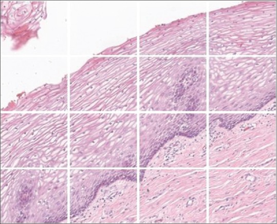
Original image split into n_r × n_c tiles

Figure 6.

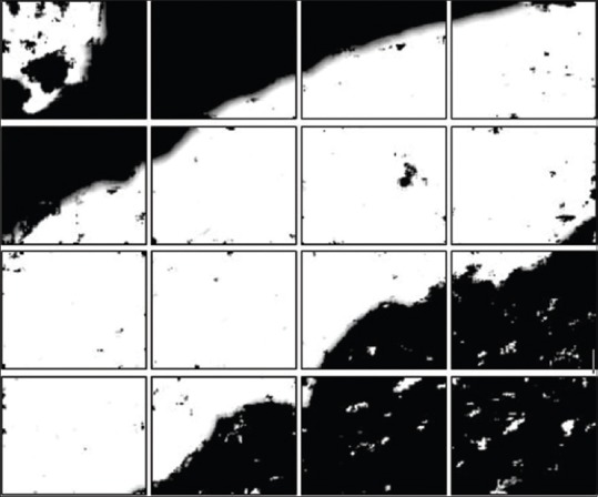
Predicted mask from each tile of original image

The generated mask tiles are later stitched using a reference label image generated during the splitting process. The resultant output mask is resized by a factor of 4 (equivalent to stride s = 4) to match the size of original input image. The output fuzzy mask is processed further to obtain a clean binary epithelial segmentation mask.

Postprocessing

Postprocessing includes the removal of unwanted noise in the mask and smoothing the edges of the segmentation. In the epithelial mask generation, there is always a problem of drawing an exact boundary even by an expert pathologist. Considering this situation, we created a model that can generate a gradient mask; this gives us ability to choose an appropriate threshold that can satisfy the pathologist conditions. We choose values between 0.35 and 0.5 as an optimal threshold range, obtained empirically. By default, we consider 0.5 as our threshold. Since the epithelial region covers most of the image area, thresholding with this value is applied to retain the object with maximum area in the image; the remaining image area is masked as background.

The edges in the mask appear to be abruptly changing, as shown in Figure 7a, and smoothing of the edge contour is accomplished by approximating a Bezier curve. This is a parametric curve controlled by Bezier control points. The Bernstein polynomial forms the basis of the curve. We converted the contour of the segmentation mask, which is a continuous curve, into r point data. The end of the point data is appended with the first two data points which help in closing the curve smoothly. The mid-points for every set of adjacent points were calculated and included in the data points. The updated point data are of length 2 (r + 1) + 1. A quadratic Bezier curve[17] is approximated by plotting a piece-wise continuous curve using three sets of control points iteratively using Equation 3.

Figure 7.

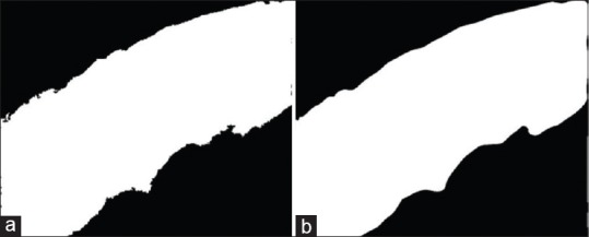
Postprocessing: (a) clean mask and (b) mask edge smoothing

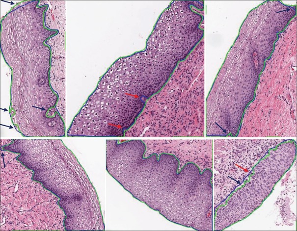
where t ∈[0,1] and i ∈[0, 2(r +1) -1]. The final curve is converted into a binary mask, as shown in Figure 7b. The resultant output mask covers the entire epithelium region and segments the region with high accuracy. This can be clearly observed from Figure 8. The green contour depicts the model predicted epithelial region, and the blue contour represents the manually drawn epithelial ground truth. The pseudo-code for the proposed pipeline is presented in Algorithm 1.

Figure 8.

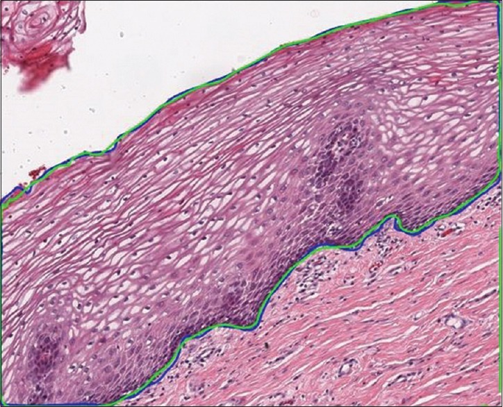
Segmentation contour

Algorithm 1.

Epithelial segmentation

Preprocess

Generate (n,m) patches with stride s

Calculate the respective ground-truth probabilities

Train

Initialize weights and bias

For i=1: N_epochs, do

Forward pass, predict

L1 Loss:

Backpropagate,

Update weights with Adadelta optimizer:

End for

Save model and weights

Test

Load model and weights

Pad image:

Slice image to p,q subimages,

Generate (n,m) patches with stride 4

Predict the probability of each pixel

Combine the predictions to form a gradient mask

Upscale the mask by factor of 4

Post-process

Threshold the mask

Smooth the mask edges with quadratic Bezier curve,

EXPERIMENTS

We performed the following experiments on the epithelium set: high-resolution cervical histology microscopy images (×10). Since we have abundant image data, we do not incorporate leave-one-out methodology in our approach. The available 351 cervical histology images were divided into disjoint training and test sets. A set of 40 images, 10 from each class, were considered as training images, as previously described, with the remaining 311 images utilized for testing. The models were tested with various color spaces: RGB, LAB, HSV, and YCrCb, also with individual and combinations of color spaces. EpithNet models were observed to perform better with the normalized RGB images than other color spaces. The normalization is performed by dividing every pixel by the brightest pixel intensity of the image, and the images were split into smaller patches to create a large dataset with a standard size. The images are split into overlapping patches forming our training set with 254,514 subimages, and the test set is dependent on the epithelial image under test since each image has different dimensions, hence changing the number of subimages obtained from the epithelial image.

Experimental models

We developed three models: EpithNet-16, EpithNet-32, and EpithNet-64. Each model is fed with different spatially localized images of sizes 16 × 16, 32 × 32, and 64 × 64, respectively. The models also vary in depth of six, seven, and eight layers, respectively. We observed that the model with higher spatial information about a pixel’s surroundings has better knowledge with more feature information and can better predict the pixel’s behavior. This is clearly evident from Table 1. As a step toward improving the segmentation accuracy, we have combined all three proposed models with internal interactions, as shown in Figure 9, and named the model as EpithNet-mc (mc denotes multicrop).

Table 1.

Results on 311 cervical histology test data

Model	J	DSC	PA	MI	FWI
UNet-64
Median	0.738	0.849	0.845	0.709	0.740
Mean	0.676	0.789	0.822	0.692	0.712
SD	0.190	0.160	0.116	0.153	0.154
EpithNet-16
Median	0.939	0.969	0.965	0.959	0.921
Mean	0.915	0.954	0.951	0.943	0.897
SD	0.070	0.043	0.045	0.049	0.081
EpithNet-32
Median	0.947	0.973	0.970	0.966	0.933
Mean	0.931	0.964	0.961	0.954	0.916
SD	0.049	0.028	0.029	0.037	0.059
EpithNet-64
Median	0.950	0.974	0.972	0.939	0.945
Mean	0.935	0.966	0.963	0.920	0.930
SD	0.049	0.028	0.032	0.062	0.054
EpithNet-mc
Median	0.952	0.976	0.974	0.942	0.949
Mean	0.940	0.969	0.966	0.926	0.936
SD	0.041	0.023	0.026	0.052	0.046

SD: Standard deviation, J: Jaccard index, DSC: Dice score, PA: Pixel accuracy, MI: Mean intersection over union, FWI: Frequency-weighted intersection over union

Figure 9.

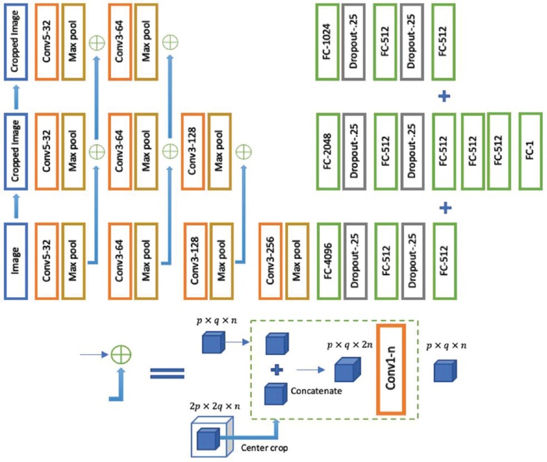
EpithNet-mc architecture

The EpithNet-mc model is designed to read an input image of size 64 × 64, and at each layer, the input image at the first layer and the feature maps in the hidden layers are center cropped such that an array of size p × q × n is extracted from an array of size 2p × 2q × n. These cropped versions of feature maps are concatenated with the feature maps from the low-resolution CNN model running in parallel. The dimensions of the concatenated feature maps are lowered by applying a 1 × 1 convolutional filter. This reduces the dimensions of the feature maps while retaining salient features. The features coming from the high-resolution CNN have better feature information with additional knowledge of the spatial data, especially on the edges.

We compare EpithNet-16, EpithNet-32, EpithNet-64, and EpithNet-mc with U-Net,[11] which is a state-of-the-art transfer network model for image segmentation in the field of biomedical imaging. We modified U-Net to make it capable of reading 64 × 64 patch image data with the same set of subimages subjected to training by EpithNet-64 to form our new baseline and named as UNet-64 with a structure containing 24 convolutional layers. UNet-64 is trained for 300 epochs with an Adam optimizer with a learning rate of 0.0001 under early stopping conditions. U-Net is a fully convolutional neural network (FCN) and generates an output mask of size equal to the input image; the ground truths are the masks of the corresponding patch image data. In the testing phase, the image is split into a grid of nonoverlapping 64 × 64 subimages which are fed to the model to predict their corresponding masks. These masks are stitched together to form a binary segmentation mask equal to the size of the original image.

The complexity of the UNet-64 model (24 layers) is over 31 million trainable parameters [Table 2]. In contrast, fewer parameters are present in EpithNet-16 (6 layers), EpithNet-32 (7 layers), EpithNet-64 (8 layers), and EpithNet-mc (21 layers), with only 1.07 million, 1.66 million, 3.01 million, and 6.85 million, respectively.

Table 2.

Complexity of baseline, UNet-64, and the proposed models

Model	UNet-64	EpithNet-16	EpithNet-32	EpithNet-64	EpithNet-mc
Parameters (×106)	31.032	1.071	1.669	3.013	6.856

Experimental results

The image segmentation is evaluated using the following metrics:

where X and Y denote the binary masks of ground truth and predictions, respectively; TP is the number of true positives denoting the pixels correctly identified as epithelium; TN is the number of true negatives that indicate the pixels correctly identified as background pixels; FP is the number of false positives indicating background pixels that are incorrectly identified as part of epithelium; FN is the number of false negatives indicating epithelium pixels mislabeled as background pixels; n_ji represents the number of pixels of class j predicted that actually belong to class i; and t_i denotes the total number of pixels of class i in the ground-truth mask. The equations (4)-(8) represent Jaccard index, J; Dice score, DSC; pixel accuracy, PA; mean intersection over union (IOU), MI; and frequency-weighted IOU, FWI, respectively. Jaccard index is defined as the number of pixels in the intersection of the two masks divided by union of pixels among the two masks. The Dice score is twice the number of common pixels divided by sum of pixel counts for both masks. Both Jaccard index and Dice score are the best descriptors of similarity coefficients between two masks and have been used in international segmentation challenges.[18] Pixel accuracy represents the percentage of pixels that were classified correctly. Mean IOU and frequency-weighted IOU are measures of object detector accuracy. These metrics are more effective with multiclass segmentation problem settings even when the classes are imbalanced. PA, MI, and FWI are the metrics considered for semantic segmentation and scene parsing.[19] All metrics penalize both false-positive and false-negative segmentation errors.

The models, trained on patch image data generated from 40 original images, produced state-of-the-art segmentation results when tested on the 311 unseen image samples. The results indicate that the proposed models have performed better than the UNet-64 model on all the test images [Table 1].

DISCUSSION

We observe from Table 1 that the proposed EpithNet models outperform the baseline UNet-64 model. EpithNet-16, EpithNet-32, and EpithNet-64 are smaller CNN models with EpithNet-16 having 31 times fewer parameters than the UNet-64 model [Table 2]. High-resolution models such as 64 × 64 with EpithNet-64 have better segmentation results. This can be clearly understood from the fact that the model can have a better awareness of its spatial environment with a high-resolution image which gives the ability to better judge the probability of the central pixel being an epithelium pixel. The multicrop EpithNet (EpithNet-mc) model was found to improve the segmentation performance by 0.5% across all the metrics. The improvement is small, but the intermediate connections from high-resolution CNN models to low-resolution CNN models help the combined model by providing better feature information across the low-resolution CNNs.

Our baseline model, UNet-64, is found to learn features without overfitting, but during the testing phase, the model performed worse. This may be due to patch data which contain images where there is a complete epithelium region, complete background, or the edge regions which contain both epithelium and background. Since the U-Net model is trained with a loss function that gives additional weight to the pixels at the border of the segmented objects, the images with complete epithelium or complete background confuse the model while learning features. The only advantage with the UNet-64 compared to EpithNet models is the shorter time taken to predict and generate a full binary mask. Despite having so many parameters, UNet-64 is an FCN which generates a binary mask of size equal to the input image, whereas the EpithNet models predict the probability of individual pixels, which ultimately takes more time to predict the mask.

Due to limited histology data availability and problems with varying image sizes, the proposed EpithNet models are the best choice; this is clearly evident from the segmentation results. The distribution of the metric values for test results on our best model (EpithNet-mc) can be visualized from Figure 10.

Figure 10.

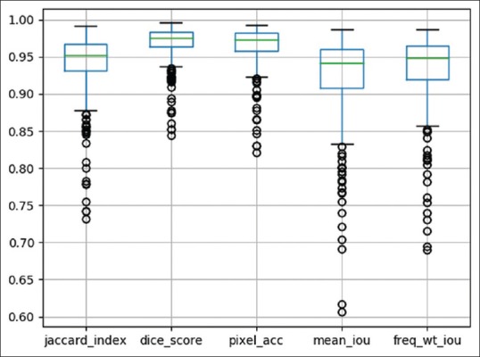
Boxplot of EpithNet-mc model with distribution of the metrics on 311 images. The column parameters from left to right indicate Jaccard index, Dice score, pixel accuracy, mean intersection over union, and frequency-weighted intersection over union. See equations (4)–(8) above with accompanying parameter descriptions

Figure 11 shows some of the promising segmentation results of the epithelial regions from the test dataset. The segmentation at the edges fairly accurately tracks the ground-truth edges. The model that generated the fuzzy mask is thresholded at 0.5 (empirically chosen as the optimum value), that is, pixel intensities >0.5 are considered as epithelial region and below 0.5 as background. It can also be observed from Figure 11 marked with blue arrows that sometimes the prediction masks do a better job in segmenting the epithelium accurately compared to the manually drawn ground-truth masks. The automated segmentation tries to discard the regions that look similar to lamina propria or red blood cells near the edges and tries to include the epithelium regions, thereby correcting the manually drawn masks.

Figure 11.

Segmentation results. Green contour represents the predicted mask and blue contour represents the ground-truth mask. The blue arrows point to regions where the predicted masks do a better job in segmenting the epithelium regions compared to the manually drawn borders. The red arrows indicate regions of false segmentation

There were few exceptional cases that segmented a major portion of the epithelium region with small areas of false identification of the edges due to large variation in the staining and pattern of the nuclei looking similar to the nuclei in the stroma region below the epithelium. Sometimes, the technique tries to remove the red blood cells even at the cost of missing epithelial regions. This can be observed from the red arrows in Figure 11.

CONCLUSION

We propose an approach to segment epithelial regions from a set of sparse epithelial data. Challenges in segmentation of histology images include variable staining, and noise including extravasated red blood cells and stain blobs, along with a limited number of ground-truth images. The techniques here offer a deep learning approach to meet the difficult challenge of architectural segmentation in automated histopathology. Reproducing the high-level approach of the expert pathologist is difficult. This article proposes a DL approach for architectural feature detection to replace handcrafted techniques that have been employed for such features.[20]

The major contribution of this work is proposing a set of patch-based epithelium segmenting regression models yielding segmentation accuracy exceeding state-of-the-art results. We use a split-and-join scheme to optimally use the available memory during the testing phase and postprocessing techniques to generate a smooth border using Bezier curves. The proposed EpithNet models are smaller and simpler but efficient in segmenting the epithelial regions of the cervical histology images. The generated mask is a probability mask, allowing the user to adjust the probability threshold to finely adjust the binary mask as needed. The results were reported by considering a default threshold value of 0.5. Moreover, it is observed from the results that the more the spatial information around a pixel is presented to the model, the better the segmentation masks generated, especially at the critical borders of the epithelium regions. EpithNet-mc was designed to combine the feature information from EpithNet-16, EpithNet-32, and EpithNet-64, which read image patches of varying spatial information centered at a given pixel. The features from layers carrying lower spatial dimensions were concatenated with features from layers carrying higher spatial dimensions to improve the quality of feature information, which ultimately resulted in generation of better segmentation masks. Although the baseline UNet-64 model, a fully convolutional network, is faster in generating the segmentation masks, the quality of the masks was poor. EpithNet, in contrast, not only generated relatively better epithelium masks but also utilized fewer parameters, resulting in less GPU memory use.

The proposed models can also help in segmenting other epithelial tissues in pathology studies. Training these models with respective histology images would help in more accurate epithelium segmentation during the testing phase. The results of segmentation of digital slides captured with different scanners and at varying resolutions is a subject for future research.

In future work, the proposed models will be used to generate the epithelium masks on digitized histology images at ×10. These segmented regions will be further analyzed to ultimately create a classification model that can better estimate the severity of cervical cancer by image processing. This could serve as a useful assistance tool for pathologists in segmenting out the useful regions and classifying the CIN levels while examining the samples.

Financial support and sponsorship

This research was supported (in part) by the Intramural Research Program of the National Institutes of Health, National Library of Medicine, and Lister Hill National Center for Biomedical Communications. In addition, we gratefully acknowledge the medical expertise and collaboration of Dr. Mark Schiffman and Dr. Nicolas Wentzensen, both of the National Cancer Institute’s Division of Cancer Epidemiology and Genetics.

Conflicts of interest

There are no conflicts of interest.

REFERENCES

- 1.Global Cancer Observatory: Cancer Today. World Health Organization; 2018. [Last accessed on 2019 Aug 21]. International Agency for Research on Cancer. Available from: https://www.who.int/cancer/prevention/diagnosis-screening/cervicalcancer/en/ [Google Scholar]
- 2.Erickson BA, Olawaiye AB, Bermudez A. Cervix uteri. In: Schilsky RL, Gaspar LE, Washington MK, Sullivan DC, Brierley JD, Balch CM, et al., editors. AJCC Cancer Staging Manual. 8th ed. 52. New York: Springer; 2017. [Google Scholar]
- 3.Jeronimo J, Schiffman M, Long LR, Neve L, Antani S. 17th IEEE Symposium on Computer-Based Medical Systems: IEEE Computer Society. Bethesda: IEEE Computer Society; 2004. A tool for collection of region based data from uterine cervix images for correlation of visual and clinical variables related to cervical neoplasia; pp. 558–62. [Google Scholar]
- 4.Kumar V, Abba A, Fausto N, Aster J. Robbins and Cotran Pathologic Basis of Disease. 9th ed. 22. Vol. 22. Philadelphia: Elsevier Saunders; 2014. The female genital tract; p. 1408. [Google Scholar]
- 5.He L, Long LR, Antani S, Thoma GR. Sequence and Genome Analysis: Methods and Applications. Vol. 15. Hong Kong: Concept Press; 2011. Computer assisted diagnosis in histopathology; pp. 271–87. [Google Scholar]
- 6.Wang Y, Crookes D, Eldin OS, Wang S, Hamilton P, Diamond J. Assisted diagnosis of cervical intraepithelial neoplasia (CIN) IEEE J Sel Top Signal Process. 2009;3:112–21. [Google Scholar]
- 7.Stanley RJ, Lu C, Long R, Antani S, Thoma G, Zuna R. A fusion-based approach for uterine cervical cancer histology image classification. Comput Med Imaging Graph. 2013;37:475–87. doi: 10.1016/j.compmedimag.2013.08.001. [DOI] [PMC free article] [PubMed] [Google Scholar]
- 8.Guo P, Banerjee K, Joe Stanley R, Long R, Antani S, Thoma G, et al. Nuclei-based features for uterine cervical cancer histology image analysis with fusion-based classification. IEEE J Biomed Health Inform. 2016;20:1595–607. doi: 10.1109/JBHI.2015.2483318. [DOI] [PMC free article] [PubMed] [Google Scholar]
- 9.Wang Y, Crookes D, Diamond J, Hamilton P, Turner R. 2007 29th Annual International Conference of the IEEE Engineering in Medicine and Biology Society. Lyon: IEEE; 2007. Segmentation of squamous epithelium from ultra-large cervical histological virtual slides; pp. 775–8. [DOI] [PubMed] [Google Scholar]
- 10.Wassmer F, De Luca V, Casanova R, Soltermann A, Székely G. 2016 IEEE 13th International Symposium on Biomedical Imaging (ISBI) Prague: IEEE; 2016. Automatic segmentation of lung carcinoma in histological images using a visual dictionary; pp. 1037–40. [Google Scholar]
- 11.Loncova Z, Hargas L, Koniar D. Segmentation of microscopic medical images using local binary patterns method. Proceedings of the 8th International Conference on Signal Processing Systems. 2016:36–40. [Google Scholar]
- 12.Ronneberger O, Fischer P, Brox T. U-Net: Convolutional networks for biomedical image segmentation. Medical Image Computing and Computer-Assisted Intervention – MICCAI 2015: 18th International Conference, Munich, Germany, October 5-9, 2015, Proceedings. In: Navab N, Hornegger J, Wells WM, Frangi AF, editors. Part III. Cham: Springer International Publishing; 2015. pp. 234–41. [Google Scholar]
- 13.Simonyan K, Zisserman A. Very Deep Convolutional Networks for Large-Scale Image Recognition arXiv, vol abs/14091556. 2015 [Google Scholar]
- 14.Nair V, Hinton GE. Haifa, Israel: 2010. Rectified linear units improve restricted Boltzmann machines Proceedings of the 27th International Conference on Machine Learning; pp. 807–14. [Google Scholar]
- 15.Maas AL, Hannun AY, Ng AY. Vol. 28. Atlanta: ICML; 2013. Rectifier nonlinearities improve neural network acoustic models Proceedings of the 30th International Conference on Machine Learning; p. 6. [Google Scholar]
- 16.Zeiler MD. ADADELTA: An Adaptive Learning Rate Method arXiv Vol abs/12125. 2012 [Google Scholar]
- 17.Hazewinkel M. Mathematics for Computer Graphics Applications. 2nd ed. New York: Industrial Press Inc; 1999. The Bezier curve; p. 264. [Google Scholar]
- 18.Codella NC, Gutman D, Celebi ME. Skin Lesion Analysis Toward Melanoma Detection: A Challenge at the 2017 International Symposium on Biomedical Imaging (ISBI), Hosted by the International Skin Imaging Collaboration (ISIC) ArXivorg>cs>arXiv:171005006; 2017. [Last accessed on 2019 Jul 24]. Available from: https://arxivorg/abs/171005006 .
- 19.Shelhamer E, Long J, Darrell T. Fully convolutional networks for semantic segmentation. IEEE Trans Pattern Anal Mach Intell. 2017;39:640–51. doi: 10.1109/TPAMI.2016.2572683. [DOI] [PubMed] [Google Scholar]
- 20.Arevalo J, Cruz-Roa A, Arias V, Romero E, González FA. An unsupervised feature learning framework for basal cell carcinoma image analysis. Artif Intell Med. 2015;64:131–45. doi: 10.1016/j.artmed.2015.04.004. [DOI] [PubMed] [Google Scholar]