A flow-chart for developing water quality criteria from two field-based methods

Abstract

Field-based methods increase relevance and realism when setting water quality criteria. They also pose challenges. To enable a consistent process, a flow chart was developed for choosing between two field-based methods and then selecting among candidate results. The two field-based methods estimated specific conductivity (SC) levels likely to extirpate 5% of benthic invertebrate genera: an extirpation concentration distribution (XCD) method and a background-to-criterion (B-C) model developed by the U.S. Environmental Protection Agency. The B-C model is a least squares regression of the 5th centile of XCD (XCD₀₅) values against estimates of background SC. Selection of an XCD₀₅ from the flowchart is determined by characteristics of the paired chemical and biological data sets and method for estimating the XCD₀₅ values. Confidence in these example SC XCD₀₅ values is based on the size of the data sets and ecoregional SC disturbance. The level of ecoregional SC disturbance was judged by comparing the background SC (the 25th centile of the data set used to calculate a XCD₀₅) and an estimate of natural base-flow SC modeled from geophysical attributes in the region. The B-C approach appears to be a viable option for estimating a SC benchmark with inexpensive estimates of SC background while the XCD method is used when the data are abundant. To illustrate the use of the flow chart, example SC XCD₀₅ values were calculated for 63 of 86 Level III ecoregions in the conterminous United States of America.

Graphical Abstract

1. Introduction

Protection and restoration of conditions that support aquatic life have typically relied upon regulatory criteria, standards, and other benchmarks based on laboratory tests (Stephan et al., 1985; CCME, 2007; Van Vlaardingen and Verbruggen, 2007; European Commission, 2011; Warne et al., 2015). However, in 2011, the United States Environmental Protection Agency (U.S. EPA) released a field-based extirpation concentration (XC₉₅) distribution (XCD) method for developing a benchmark for specific conductivity (SC) (U.S. EPA 2011, Cormier and Suter 2013).

SC was selected for development of the XCD method because a strong body of science has demonstrated the significant impacts of elevated SC on aquatic life and the communities that depend on freshwater streams for drinking, fishing, industry, agriculture and animal husbandry, recreation, and other uses (ECHC 2001; Cañedo-Argüelles et al., 2013; Kaushal et al., 2013). SC, a measure of dissolved ions (salts) in water, has been identified in the peer reviewed scientific literature as one of the key measures of stream condition and is widely measured along with pH and temperature.

Aquatic life impairments linked to elevated SC are widespread (ECHC 2001; Cañedo Argüelles et al., 2013; Kaushal et al., 2013). Many sources are man-made (Griffith 2017) and thus controllable with best management practices for resource extraction (mining, oil and gas development and production), urban development, irrigation return water, and industrial wastewater discharges. In the USA, there is currently a patchwork of state/tribal water quality standards for dissolved salts. These criteria are generally set at some percentage (e.g. 33–50%) above “background,” and may not be based on effects or risk to aquatic life. Data sets developed over the last 20 years open the door to newer methods based on the relationship between elevated conductivity and adverse effects measured in the field. A recommended methodology that represents strong peer-reviewed science can provide a basis for addressing ionic contamination and its effects.

Although the XCD method is applicable to any area with a well-defined ionic mixture and large suitable data sets, only one benchmark from a large data set from central Appalachia was derived as an example (U.S. EPA, 2011). The method has also been applied in at least one other location in China (Zhao et al., 2016). A disadvantage of the method is that it requires at least 500 paired biological and chemical samples that also include levels of SC that are harmful to salt-intolerant organisms. These requirements have been limiting factors for more widespread adoption of field-based methods for developing water quality criteria.

Because large sets of paired chemical and biological data are not available for many places, less data-intensive methods are needed. One option is to develop chronic criteria for defined geographical areas using background SC and a background-to-criterion (B-C) regression model (Cormier et al., 2018a). This approach is useful for areas lacking sufficient paired biological and SC data to use the XCD method. Moreover, this B-C model enables the development of protective field-based benchmarks or criteria before exposures have reached concentrations extirpating 5% of taxa (XCD₀₅) in water bodies.

The B-C model characterizes a relationship between background SC and XCD₀₅ values (Cormier et al., 2018a]). XCD₀₅ values were estimated at the 5th centile of 24 genus-level XCDs. Those 24 XCD₀₅ values were regressed against background SC values, estimated as the 25th centile SC for each data set. XCDs were developed for ecoregions with background SC values from 22 to 626 μS/cm. In general, as background SC increases, the most salt-intolerant genera in an ecoregion occur at progressively higher SC levels, and the 5th centile of the XCD occurs at a higher SC. This is predictable because salt-intolerant taxa with XC₉₅ values less than background are not likely to contribute to the XCD, but taxa with an XC₉₅ greater than background are likely to survive and contribute to the XCD. The association from the linear regression is strong and not surprising, because all aquatic taxa have physiological limitations and optima at particular ionic conditions (Remane, 1971; Bos et al., 1996; Potapova and Charles 2003; Kefford et al., 2004, Potapova, 2005; Berra, 2007; U.S., EPA 2011; Olson and Hawkins, 2012; Cormier et al., 2013; Vander Laan et al., 2013).

In this paper, a decision flowchart is described for choosing a method for developing a benchmark or criterion for SC. The two methods are the original field-based XCD method (Cormier and Suter, 2013; U.S. EPA, 2011) and the field-based B-C model method (Cormier et al., 2018a; U.S. EPA, 2016). The decision flowchart is used to derive example XCD₀₅ values for 63 of the 85 Level III ecoregions in the conterminous United States. These example XCD₀₅ values illustrate commonly encountered issues of data set size, ionic mixture incompatibility, model range reliability, within-ecoregion variability, and uncertainty regarding the independent variable used is some estimates.

2. Methods

2.1. Decision flowchart

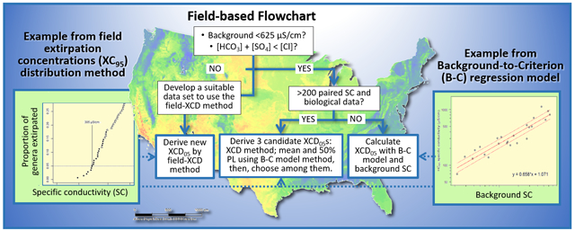
A flowchart was designed to help guide reasonable judgments for protectiveness while being mindful of the uncertainties associated with derivation methods and sample sizes. In this flowchart, the choice of XCD₀₅ is from among the 5th centile of an XCD, the mean modeled XCD₀₅ from the B-C regression model, the lower 50% prediction limit (PL) from the B-C model, or no result. Other factors associated with a data set or ecoregion, such as the level of ecoregional disturbance or variability, were also important considerations and are described separately.

The first step recommends that the area is assessed in terms of its consistency of background SC (Fig. 1, Step A). All of the examples were performed at the Level III Ecoregion scale (Omernik 1987). An ecoregion is considered a relatively homogeneous geographical area delineated by attributes such as climate, physiography, geology, soils, vegetation, and water resources (McMahon et al., 2001). Because the Level III ecoregions are not defined solely on the basis of background SC, it is advisable to evaluate whether there are distinct areas within an ecoregion that have biologically relevant differences in natural background. In the example uses of the flowchart, a geophysical model was used to identify discontinuities in modeled natural background SC (Appendix A1; Olson and Hawkins, 2012). Because background SC differed by at least 50 μS/cm in all ecoregions, the selection of a cutoff value for variability of background across an ecoregion was based on practical constraints as well as on a range of acceptable biological effects. Background for each ecoregion was estimated with a geophysical model that predicts mean base flow stream SC (Olson and Hawkins, 2012). Background was considered too variable when the mean modeled SC of >20% of stream-kilometers varied by more than 200 μS/cm within an ecoregion. Thus, the result is a screening level threshold that is expected to avoid the most serious effects with improved resolution of the example water quality criteria dependent on estimates of background SC and a more precise XCD₀₅.

Figure 1.

A decision flowchart for calculating and applying 5th centile of the extirpation concentration distribution (XCD₀₅). Lettered product paths are described in the body of the text. extirpation concentration distribution (XCD); background-to-criteria (B-C); specific conductivity (SC); Prediction limit (PL).

Once the area for analysis is defined, the available data set is evaluated to determine whether to use the field-based XCD method or to use the B-C model (Fig. 1, steps B, C). Characteristics of suitable data sets for the XCD method include taxonomic identification to genus, similar ionic mixture, and some samples >1000 μS/cm (U.S. EPA, 2016). Sensitivity analyses indicate that a sample size of ≥500 sites may be sufficient to develop an XCD₀₅ using the field-based XCD method if ≥5% of XC₉₅ values unambiguously occur in the sampled SC range. A representative sensitivity analysis is described in Section 2.2. If these conditions are met, the XCD₀₅ is calculated by the XCD method (Fig. 1, steps F, L). The B-C model is used only within the range of the model (Fig. 1, step C). The B-C method may be used where the background SC is within the range of the model: less than 625 μS/cm and the ionic mixture is similar, that is, ([HCO₃⁻] + [SO₄²⁻]) > [Cl⁻] in mg/L. If either condition is not met, then a suitable data set needs to be developed so that the XCD method can be used, because a B-C model is not yet available for mixtures dominated by chloride anions (Fig. 1, steps D, F, L).

The rest of the decision flowchart describes how to choose the XCD₀₅ from the mean or the lower PL of the B-C modeled XCD₀₅ or an XCD₀₅ developed using the XCD method with a small data set. Where there are <200 paired biological and SC data (Fig. 1, step E), the XCD₀₅ and lower 50% PL is calculated from the B-C model and background SC (Fig. 1, step H). The lower 50% PL as the XCD₀₅ (Fig. 1, step O) is recommended because the method relies only on the B-C model with no corroboration with another method and therefore the more conservative value is appropriate.

When there are >200 and <500 paired SC and biological data, 3 candidate XCD₀₅ values are calculated and compared (Fig. 1, step E). One estimate is generated from the XCD method and the other two are the modeled mean and its lower 50% PL calculated from the B-C model (Fig. 1, step G). These values are compared to select an XCD₀₅ as shown in steps I, J, K (Fig. 1). The recommended selection is as follows: (1) If the XCD XCD₀₅ (U.S. EPA, 2011) is greater than the mean B-C modeled XCD₀₅ (U.S. EPA, 2016), then the mean B-C modeled XCD₀₅ is recommend (Fig. 1, steps I and M) because there is greater uncertainty associated with smaller data sets. (2) If the XCD₀₅ is between the mean B-C modeled XCD₀₅ and the lower 50% PL, then the XCD₀₅ from measured data from the region are recommended because it may more closely represent the region than the more general B-C model result (Fig. 1, steps J, N). (3) If the XCD estimate is below the lower 50% PL, then the lower 50% PL is recommended as the XCD₀₅, because the XCD estimate is more uncertain than the modeled results (due to smaller sample size) (Fig. 1, steps K, O). Also, the definition of the PL implies that 75% of XCD₀₅ values from areas with a similar background SC will be greater than a value less than the lower 50% PL.

2.2. Sensitivity analysis of data set sample size

During development of the models, methods, and flowchart, several decisions were based on logic, expert consensus, and sensitivity analyses. One such decision was the sample size requirement for selecting between the XCD-method and the B-C method. This decision was based on the sensitivity of the XCD-method to the amount of available data. Sensitivity analysis involves changing the sample sizes used to estimate input values of the models to see the effect on the output value, which is the 5th centile of a distribution of XC₉₅ values. The effects of data set size on the XCD₀₅ estimates and their confidence bounds were estimated using bootstrapping. Bootstrapping is a statistical technique of repeated random sampling with replacement from a data set to estimate an average and confidence limits of a parameter (Newman et al., 2001, 2000). Then, the XC₉₅ for each genus was calculated from the bootstrapped data set and the XCD₀₅ was calculated. The distribution of 1000 XCD₀₅ values was used to generate two tailed 95% confidence limits on these bootstrap derived values. The process was repeated for each selected sample size ranging from 100 to the size of the full data set. The mean of all bootstrapped XCD₀₅ values, the numbers of genera used for the XCD₀₅ calculation, and their 95% confidence limits were plotted in Fig 2 using a representative data set from Central Appalachia (Ecoregion 69).

Figure 2.

The effect of the size of the data set used to model the extirpation concentration distribution (XCD) at the 5th centile (XCDC₀₅) based on the Ecoregion 69 example data set. The XCD₀₅ stabilizes reaching an asymptote at approximately 500–800 sites sampled (circles).

Large high-quality data sets are required to determine the effects of smaller sample sizes. West Virginia Department of Environment Protection data sets from the Central Appalachia (Ecoregion 69) and the Western Allegheny Plateau (Ecoregion 70) were used in these sensitivity analyses. These data included water chemistry samples (e.g. SC, pH) and biological samples identified to the genus level. Sample collection methods and sources of data sets are listed in Appendix A.

Figure 2 depicts the results of the sensitivity analysis for the effect of the number of samples in the data from the Central Appalachian Ecoregion 69. The geomean bootstrapped XCD₀₅ values between 500 and 1500 samples varied less than 35 μS/cm and the 95% CI varied by no more than 20%. Similar results were obtained for the Western Allegheny Plateau Ecoregion 70 (U.S. EPA, 2016); above 800 samples 95% CIs and XCD₀₅ values are consistent. For greatest inclusivity, 500 samples were identified as a minimal data set to calculate an XCD₀₅ with the field-based method. For a different application, that is, to compare the XCD and a B-C generated XCD₀₅, a smaller data set could be acceptable, but at a sample size of 100, the uncertainty was very large, >700 μS/cm with the Central Appalachia data set. At a sample size of 200, the 95% CI < 270 μS/cm and the uncertainty was judged to be acceptable for calculating an XCD₀₅ for comparison with a B-C XCD₀₅. The recommendation for a minimum of 200 samples can be used because the uncertainty of the XCD₀₅ value is limited by the modeled mean and the lower 50% PL of the B-C model. That is, a low sample size tends to raise the XCD₀₅, but it is not used if the result is greater than the B-C modeled mean result.

2.3. Example benchmarks

Data sets

Example water quality criterion values derived with the XCD method were calculated using various state data sets (N > 200) (U.S. EPA, 2011; Cormier and Suter, 2013; U.S. EPA, 2016). Example water quality criterion values derived with the B-C model used background SC values from state data sets and smaller U.S. EPA survey data sets compiled by Griffith (2014). In Ecoregion 4, Cascades, and Ecoregion 43, Northwestern Great Plains, data were readily available from compiled USGS data so these were combined with the other available data to estimate background SC in those ecoregions. Data sets are available from the U.S. EPA Environmental Dataset Gateway listed in Section 6. Data Availability.

Analyses

The XCD method (Cormier and Suter, 2013) and the B-C method (Cormier et al., 2018a; U.S. EPA, 2016) were used to estimate example XCD₀₅ values for 63 of the 86 Level III ecoregions in the conterminous United States of America (USA) (formulae are available in Appendix A and Cormier et al., 2018a).

The B-C method requires an estimate of background SC. The sample size for estimating the background SC was based on 30 samples. Greater confidence was assigned to background estimates based on a doubling of the convention to 60 samples (Table 1). For first approximation estimates of background and example criteria, a minimum sample size of 20 was accepted (Table 2). Ecoregions with ≤20 sites sampled for SC were not analyzed. Ecoregions were not analyzed by the B-C method when the 25th centile SC of the data set was ≥625 μS/cm. Tables 1-3 list analyzed data sets. Unanalyzed ecoregions are listed in Table 4.

Table 1.

Ecoregions with minimally affected background and >59 samples of specific conductivity (SC) measurements. Examples of 5th centile hazardous concentration (XCD₀₅) values are from extirpation concentration distribution (XCD) method, and the mean and 50% prediction limits (PL) using the background-to-criterion (B-C) method. Modeled mean base-flow SC is greater than 25th centile measured SC for all except Ecoregion 60. Figure 1 was used to select example values (gray).

		Source of Data Sets
		State data set			EPA-survey data set					Modeled
Level III ecoregion number and name		N	25th centile	XCD- Method XCD05	N	25th centile	B-C mean XCD05	B-C lower PL XCD05	B-C upper PL XCD05	Mean base-flow 25th centile
1	Coast Range	–	–	–	251	53	160	133	193	99
3	Willamette Valley	–	–	–	87	62	179	148	215	94
4	Cascadesa	–	–	–	537a	33	118	97	142	66
7	Central California Valleyb	–	–	–	82	99	243	202	291	411
11	Blue Mountains	–	–	–	135	85	219	182	263	161
15	Northern Rockies	614	29	142	29	22	89	73	108	100
16	Idaho Batholith	1040	42	185	29	36	125	103	151	81
17	Middle Rockiesb	510	136	264	89	78	208	173	249	229
19	Wasatch and Uinta Mountainsb,c	773	271	299	32	31	113	93	137	285
21	Southern Rockiesb	–	–	–	164	83	217	180	260	218
23	Arizona/New Mexico Mountainsb,c	374	191	249	38	105	253	211	303	385
35	South Central Plainsd	–	–	–	60	51	156	130	188	117
40	Central Irregular Plains	–	–	–	60	301	504	419	606	324
45	Piedmont	665	68	138	333	42	138	114	166	73
50	Northern Lakes and Forests	734	108	320	151	111	261	217	313	231
52	Driftless Areab,c	344	534	655	73	392	600	498	723	406
58	Northeastern Highlands	383	50	212	118	40	133	110	161	64
60	Northern Allegheny Plateauc	562	132	248	113	72	196	163	235	112
62	North Central Appalachians	–	–	–	131	33	118	97	142	60
65	Southeastern Plains (lower)d,e	457	38	131	241	26	100	82	121	88
65	Southeastern Plains (upper)c,d,e	501	99	243	241	26	100	82	121	88
66	Blue Ridge	322	22	69	245	16	74	60	90	59
67	Ridge and Valleyb	926	59	154	522	46	147	122	177	161
69	Central Appalachians	1661	94	305	281	46	146	121	176	94
70	Western Allegheny Plateau	2075	169	338	109	153	323	269	388	180
77	North Cascades	–	–	–	73	27	104	86	126	65
78	Klamath Mountains/California High North Coast Range	–	–	–	74	83	216	180	260	151

^aData set is a combined U.S. EPA survey and U.S. Geological Survey (USGS) data set ([data set] Cormier 2017a).

^bPredicted mean base-flow varies by more than 200 μS/cm in 20% stream segments in ecoregion.

^cDifference of >50 μS/cm between state and U.S. EPA-survey background SC suggests need for further analysis.

^d([Na⁺] + [K⁺]) > ([Ca²⁺] + [Mg²⁺]) and/or [Cl⁻] > ([SO₄²⁻] + [HCO₃⁻]) in mg/L in ≥50% of U.S. EPA-survey sample.

^eElongated ecoregion suggests need for further analysis.

Table 2.

Ecoregions with minimally affected background and 23–59 specific conductivity (SC) samples. Modeled mean base-flow SC is greater than 25th centile measured SC. Examples of 5th centile hazardous concentration (XCD₀₅) values calculated with the lower 50% prediction limit (PL) of the background-to-criterion (B-C); therefore, XCD₀₅ values are first approximations. Figure 1 was used to assign example XCD₀₅ values (gray cells).

		Sources of Data Sets
		EPA survey					Modeled
Level III ecoregion number and name		N	25th centile	B-C Mean XCD05	B-C lower PL XCD05	B-C upper PL XCD05	Mean base-flow 25th centile SC
6	Central California Foothills and Coastal Mountainsab	27	244	439	365	527	480
8	Southern California Mountainsb	45	262	460	383	552	511
9	Eastern Cascades Slopes and Foothills	45	50	155	129	187	148
10	Columbia Plateau	26	128	287	239	344	264
13	Central Basin and Rangeb	51	152	321	268	385	367
18	Wyoming Basinb	37	397	605	502	728	443
20	Colorado Plateausb	33	436	643	533	775	495
25	High Plainsb	40	359	566	470	681	452
26	Southwestern Tablelandsb	25	495	699	579	844	544
29	Cross Timbersb	23	288	489	407	588	384
36	Ouachita Mountainsa	50	22	90	74	110	102
37	Arkansas Valleya	47	32	115	95	140	163
38	Boston Mountains	26	23	93	76	113	187
42	Northwestern Glaciated Plainsb	46	342	548	455	659	421
44	Nebraska Sand Hills	34	161	333	278	400	263
63	Middle Atlantic Coastal Plain	59	93	233	194	280	96
68	Southwestern Appalachians	55	40	132	110	160	104
74	Mississippi Valley Loess Plainsa,b	26	69	191	159	230	110
75	Southern Coastal Plaina	50	52	159	132	191	109
80	Northern Basin and Rangeb	47	94	234	195	282	269
82	Acadian Plains and Hills	23	53	161	133	193	89
84	Atlantic Coastal Pine Barrensa	37	62	179	149	215	68

^a([Na⁺] + [K⁺]) > ([Ca²⁺] + [Mg²⁺]) and/or [Cl⁻] > ([SO₄²⁻] + [HCO₃⁻]) in mg/L in ≥50% of U.S. EPA-survey sample.

^bPredicted mean base-flow varies by more than 200μS/cm in 20% stream segments in ecoregion.

Table 3.

Ecoregions with least disturbed background and at least one data set with >20 specific conductivity (SC) samples. Examples of 5th centile of the extirpation concentration distribution (XCD05) where 25th centile (SC) is greater than the geophysical modeled mean base-flow suggests background represents least disturbed conditions. XCD05 calculated by XCD method and the mean and 50% prediction limits (PL) using the background-to-criterion (B-C) method. Figure 1 was used to select example XCD₀₅ values (gray).

		Sources of Data Sets
		State-survey				EPA-survey				Modeled
Level III ecoregion number and name		N	25th centile μS/cm	XCD- method XCD05 μS/cm	N	25th centile μS/cm	B-C mean XCD05 μS/cm	B-C lower PL XCD05 μS/cm	B-C upper PL XCD05 μS/cm	Mean base-flow modeled SC (μS/cm)
27	Central Great Plainsd	–	–	–	133	469	675	560	815	452
39	Ozark Highlands	–	–	–	54	362	569	472	685	278
43	Northwestern Great Plainsa,b,d	–	–	–	399b	542	742	614	897	489
47	Western Corn Belt Plainsc	473	587	934	178	480	685	568	827	349
51	North Central Hardwood Forestsc	583	325	494	35	149	317	264	381	301
54	Central Corn Belt Plainsc	469	626	813	14	465 (465–1100)	671	556	809	267
55	Eastern Corn Belt Plains	–	–	–	25	612	804	665	973	247
59	Northeastern Coastal Zonea,c	277	350	706	41	105	252	210	303	72
61	Erie Drift Plain	–	–	–	33	230	422	352	507	166
64	Northern Piedmont	710	150	227	92	114	266	222	319	101
71	Interior Plateau	336	296	479	56	299	502	417	603	236
72	Interior River Valleys and Hillsc	463	462	1127	51	384	592	491	713	264
73	Mississippi Alluvial Plaind	–	–	–	27	132	292	244	351	121
83	Eastern Great Lakes Lowlandsc,d	591	272	525	17	104 (104–1890)	250	208	300	181

^a([Na⁺] + [K⁺]) > ([Ca²⁺] + [Mg²⁺]) and/or [Cl⁻] > ([SO₄²⁻] + [HCO₃⁻]) in mg/L in ≥50% of U.S. EPA-survey sample.

^bData set is a combined U.S. EPA survey and USGS data set ([data set] U.S. EPA 2016).

^cDifference of >50 μS/cm between state and U.S. EPA-survey background SC suggests need for further analysis.

^dPredicted mean base-flow varies by more than 200μS/cm in 20% stream segments in ecoregion.

Table 4.

Uncalculated 5th centile hazardous concentrations (XCD₀₅) because there were <20 samples to estimate the 25th centile background specific conductivity (μS/cm). Ecoregion 76, the Everglades, is a unique system and is influenced by saltwater intrusion.

		Source of data
		EPA-survey		Modeled
Level III ecoregion number and name		N	SC Range	Mean base-flow SC
2	Puget Lowland	11	(50–228)	71
5	Sierra Nevadaa	18	(19.1–207)	144
12	Snake River Plaina	4	(136–582)	300
14	Mojave Basin and Rangea	2	(2860)	503
22	Arizona/New Mexico Plateaua	10	(76.9–533)	486
24	Chihuahuan Desertsa	1	(3500)	504
28	Flint Hills	18	(350–800)	472
30	Edwards Plateau	6	(372–693)	489
31	Southern Texas Plainsa	-	-	462
32	Texas Blackland Prairiesa	5	(143–849)	321
33	East Central Texas Plainsa	6	(188–1560)	254
34	Western Gulf Coastal Plain	16	(71–2046)	203
41	Canadian Rockies	7	(117–364)	138
46	Northern Glaciated Plains	21	(451–2890)	329
48	Lake Agassiz Plain Range	13	(618–2630)	341
49	Northern Minnesota Wetlands	8	(77.3–607)	256
53	Southeastern Wisconsin Till Plains Range	9	(227–1070)	388
56	Southern Michigan/Northern Indiana Drift Plains	19	(295–1140)	246
57	Huron/Erie Lake Plains	8	(336–1980)	307
76	Southern Florida Coastal Plainb	603	(1.2–4540)	183
79	Madrean Archipelagoa	-	-	401
81	Sonoran Basin and Rangea	5	(279–12300)	495
85	Southern California/Northern Baja Coasta	12	(368–4100)	566

^aPredicted mean base-flow varies by more than 200 μS/cm in 20% stream segments in ecoregion.

^bUnique system, Everglades

Estimated XCD₀₅ values were assigned using the decision flowchart (Fig. 1). The selected XCD₀₅ values were further characterized according to the methods that were used, data set size, ionic mixture, the sample size used to identify the 25th centile of the data set, and within ecoregion variability of the distribution of measured SC. The resulting values were qualified in four ways. (1) Differences of >50 μS/cm between state and U.S. EPA survey background SC were identified as warranting examination of sampling design differences between the two data sets. (2) Ecoregions were identified where more than 50% of the U.S. EPA-survey samples were dominated by ([Na+] + [K+]) and [Cl−] in mg/L. (3) Ecoregions with a geophysical modeled mean base-flow SC less than the 25th centile SC background were identified as having been estimated using least disturbed rather than minimally affected SC background (Olson and Hawkins 2012). (4) Ecoregions were identified when the base-flow modeled SC in >20% of stream-kilometers varied by more than 200 μS/cm. A description of the data sets and estimation of predicted mean base-flow SC from the geophysical model is available in Appendix A

3. Results

3.1. Predicted geophysical background during base flow

The predicted natural base-flow SC was modeled at the reach scale (Fig. 3). Mountainous regions tend to have lower background SC, the central plains and arid lands tend to have the highest, and other ecoregions have intermediate background SC. Based on the geophysical-modeled, natural mean base-flow SC, Level III ecoregions in the West encompassing areas with high SC are more variable than other ecoregions (Fig. 3). Predicted mean base-flow varied by more than 200 μS/cm in ≥20% of stream segments in 32 of 86 ecoregions (Tables 1-4). Therefore, Level III ecoregions may not be the optimal scale for applying a single benchmarks or criteria in a large part of the USA.

Figure 3.

The predicted mean natural base-flow water specific conductivity (SC) is calculated using geology, climate, soil, vegetation, topography, and other factors calibrated with reference sites (Olson and Hawkins 2012). Areas in the East and Northwest are predicted to have lower natural base-flow SC than the Southwest and mid-continent.

3.2. Characterization of Ionic Mixture

Of the 86 Level III ecoregions, 27% had insufficient SC data to estimate example XCD₀₅ values using the B-C method (Table 4). In 10 of the 63 ecoregions with sufficient data (Table 1-3), ≥50% of U.S. EPA-survey samples were dominated by NaCl ([Na⁺] + [K⁺]) > ([Ca²⁺] + [Mg²⁺]) and/or [Cl⁻] > ([SO₄²⁻] + [HCO₃⁻]) in mg/L (Tables 1-3 footnotes). The ionic composition at a site may need to be verified before a criterion could be applied in these ecoregions unless areas dominated by different ionic mixtures were already removed.

3.3. Example XCD₀₅ Values

The example calculations of SC XCD₀₅s are sorted based on the size of the data sets (Table 1, N > 59 and Table 2, N < 60) and whether the SC background was minimally affected or least-disturbed (Table 3). Minimally affected and least-disturbed background SC was judged by comparing the background SC associated with the data set used to calculate an XCD₀₅ with an estimate of natural base-flow SC modeled from geophysical attributes in the same ecoregion (Fig. 3). Least disturbed background was assessed where the 25th centile SC of a data set is greater than may be expected naturally (25th centile SC > than geophysical modeled mean base-flow SC). Of the 63 ecoregions for which example criteria were estimated by either method, the estimated background was judged to be least disturbed for 24% of them.

XCD05 values were considered more reliable where they were generated from larger data sets making it possible to compare results from the XCD and the B-C methods and where the background estimate was judged to be minimally affected (Table 1). There was sufficient paired biological and chemical data to calculate XCD05 values using both methods using 27 data sets in 26 Level III ecoregions in the conterminous USA. Where the estimated background of the ecoregion was judged to be minimally affected, the example criterion from the XCD method was recommended about 50% of the time (Table 1). However, where the estimated background of the ecoregion was judged to be least disturbed, the XCD calculated example criterion was recommended approximately 21% of the time (Table 3). Many, but not all, of the areas with least disturbed estimates of background SC are located in the central portion of the country where landscapes are highly modified for row crop agriculture.

For those ecoregions with background estimates based on small data sets (N = 20 to 59 SC samples); additional SC sampling or comparison with state data sets would strengthen these analyses (Table 2). And, 27% of ecoregions had insufficient data to estimate background (Table 4).

4. Discussion

Although field-based methods increase relevance and realism, they also pose new types of challenges for setting aquatic life criteria and restoration goals. Therefore, translating scientific information to a practical application needs to be transparent and defensible (Parker et al., 2016). One method is to develop a flowchart to depict how information is evaluated to develop a value or quantity. It is also important to document the scientific underpinning of the recommendations contained in the flowchart. An approach was described for developing a flowchart to help navigate some of these challenges while assessing candidate SC aquatic life criteria derived by the field-based XCD method (Cormier et al., 2013) and the B-C method (Cormier et al., 2018). The reasons for recommended cut points were described with accompanying documentation of the analyses or references on which those recommendations were made. In particular, information was provided regarding data set size, mixtures, within ecoregion background variability, and uncertainty regarding estimated background of the stressor. To illustrate an approach using a decision flowchart for selecting among candidate SC XCD₀₅ values, example SC XCD₀₅ values were developed that had varying reliability for 63 of 86 Level III ecoregions in the conterminous USA (Tables 1-3). The resulting examples illustrate that only half of the ecoregions have sufficient data and a relatively uniform background SC to easily apply a single ecoregional value. Most of these ecoregions are east of the Mississippi River. Even then, the variation in background SC can be greater than what would be preferred to avoid under- and over-protecting with a single value. Additional data sources from other agencies or new data collection will be needed for many areas of the USA. However, at this time, the flow chart can assist in the selection of a method for deriving a field-based XCD₀₅ given different availabilities of data and prior analytical results.

The example calculations of XCD₀₅ values for SC using the B-C method are strictly example estimates. The example XCD₀₅ values estimated with these methods represent chronic thresholds and also require a maximum threshold to be fully protective (Cormier et al., 2018b, U.S. EPA, 2016). Before using these example XCD₀₅ values, the background SC values used to derive XCD₀₅ values for an ecoregion should be assessed for reliability and representativeness of the ecoregion. This is necessary because some background estimates that were used are based on small sample sizes, and because some ecoregions are large and may have different SC regimes in discrete areas of those ecoregions (Fig. 3). If there are biologically relevant differences in background SC within an ecoregion, these areas may need to be differentiated from one another and independent calculations performed to yield appropriate XCD₀₅ values. Another solution may be to develop conductivity regions rather than repurpose previously developed ecoregions. A geophysical model similar to the one developed by Olson and Hawkins (2012) could be used to identify discontinuities in modeled natural background SC, define areas with similar background SC, and develop a distinct XCD₀₅ for each similar area.

Developing XCD₀₅ values for the arid areas of the country are more challenging due to smaller data sets, naturally high SC, and greater variability of background SC. And yet, these are the areas where fresh water for all uses are most limited. Societal goals regarding allocation of scarce freshwater resources may be informed by comparing the predicted mean SC with instream measured SC.

It is important to consider the consequences of using least-disturbed background SC as the basis for deriving a benchmark or criterion (Table 3). Because the biota may already be affected by high SC in altered landscapes, derived XCD₀₅ values may be protective of remaining taxa but may not be protective of the native and therefore potential biota in the ecoregion. Awareness of the level of modification may warrant special protection of any remaining low SC waters and, if feasible, development of management practices to restore a more natural ionic regime. More extensive assessment of least disturbed conditions may be evaluated by a weight-of-evidence analysis (Cormier et al., 2018d).

Several factors may contribute to the differences between measured and geophysically modeled background SC developed by Olson and Hawkins (2012). The 25th centile SC from state and U.S. EPA survey data sets included all flow conditions whereas the geophysical model only estimates mean base-flow. Typically, stream SC is lower with the addition of surface runoff, but not necessarily in arid areas where precipitation mobilizes salts. The geophysical model estimates base-flow SC which is more likely to occur during drier months when stream SC can be higher. This occurs because ground water has greater contact with soluble minerals and because evapotranspiration concentrates minerals in soil. Also, the predicted base-flow estimates are stream-length-weighted means whereas the measured SC background estimates are 25th centiles. And lastly, the geophysical model was developed for a broad range of SC and as a result it tends to overestimate the base flow SC in the low range.

The B-C regression model was developed using biological data paired with SC data from waters where regional background SC did not exceed 626 μS/cm. Extrapolating beyond the background SC range used to develop the model should be avoided. Furthermore, the model has been tested with few ionic mixtures; and therefore, the relevance of these values needs to be assessed before using them for other ionic mixtures. Based on laboratory tests, waters dominated by NaCl may be less toxic than bicarbonate and sulfate salts (Dunlop et al., 2005; Nelson and Cox, 2005; Zalizniak 366 et al., 2006; Bradley, 2009; van Dam et al., 2014; Johnson et al., 2015; Erickson et al., 2017; Mount et al., 2016). However, the B-C model may be defensible for ionic mixtures dominated by sodium, sulfate, and bicarbonate ions because the toxicity of these mixtures is more similar to that of calcium, magnesium, sulfate and bicarbonate ions than to NaCl (Kunz et al., 2013; Soucek and Dickinson, 2015; Mount et al., 2016).

Although not evaluated in this paper, the B-C method may be applicable for fine tuning assessments to areas smaller than ecoregions or developing basin or stream-reach benchmarks and criteria. The B-C method also overcomes a disadvantage of the XCD method for which significant exposure and damage in a system must already have occurred in order to model an extirpation stressor-response relationship. For example, monitoring data show that many areas in the Pacific Northwest have very low SC (Cormier et al., 2018c) and so the needed range of SC to use the XCD-method is insufficient. The B-C method provides a means of estimating a protective criterion before damage is done. The B-C approach also appears to be a viable option for calculating a SC XCD₀₅ with inexpensive estimates of background SC thus overcoming the need for large sets of paired biological and chemical data.

5. Conclusion

In 2013, we published a method for estimating SC effect levels and provided only one example case study in the eastern USA (Cormier and Suter, 2013; Cormier et al. 2013). The method recommended that having data sets with a minimum of 500 paired biological and chemical samples that also included conditions that are well above natural background levels. Others have used this method with smaller data sets in China 388 (Zhao et al. 2016) and in Australia (van Dam personal communication). In this special section, we described an alternative method that requires less data (Cormier et al. 2018a). The B-C method appears to be applicable anywhere background SC can be estimated and therefore may be very useful with sparsely measured data. A well-developed system for choosing between these methods is needed to ensure reasoned consistency prior to application. This paper describes where it may be advisable to use one or the other method.

The example criteria illustrate commonly encountered issues of data set size limitations, ionic mixture differences, model range reliability, within-ecoregion variability, and uncertainty regarding estimates of the independent variable used in the B-C model, i.e., background SC. These field-based methods could be invaluable for setting water quality criteria for dissolved salts.

6. Data Availability

Data sets and individual XCD results used to develop the B-C model are available at the U.S. EPA Environmental Dataset Gateway (https://doi.org/10.23719/1371707) ([dataset]Cormier 2017a). Data are contained in three zip files. The folder “Biological.zip” contains occurrences of benthic invertebrate genera in 12 state data sets. The folder “Environmental.zip” contains environmental data sorted into 24 data sets. The folder “model.zip” contains the calculated XC₉₅ values, probability of observation plots as generalized additive models, and the CFD for benthic invertebrate genera from the 24 data sets used to develop the B-C model. The combined state and USGS data for Ecoregion 4, the Cascades, are available at https://doi.org/10.23719/1396168 ([dataset]Cormier 2017b). Data set for Ecoregion 43 are available in file “Eco43_SC_Ions_v5_all.csv” in the data set at https://www.epa.gov/sites/production/files/2016-12/field-based-conductivity-field-data sets.zip ([dataset]U.S. EPA 2016). Data sets for Figure 3 are described in Appendix A, Table A.1. EPA survey data set from ([dataset] Cormier, 2017c) from Griffith (2014) are available at https://doi.org/10.23719/137106.

A spread sheet for calculating XC₉₅ values and XCD₀₅ are described in Cormier et al. (2018). The tools, data sets, example calculations, and example outputs are available online at https://wiley.figshare.com/ieam and https://github.com/smcormier/Biological-Extirpation-Analysis-Tools-BEAT/releases/tag/v.1.0.2.

Similarly, calculation of XC95, GAM plots, XCD05 can be calculated using batch R-code. The R-code and data sets are available on GitHub (https://github.com/leppott/XC95).

Post publication note: Since 2012, a new model was developed (Olson and Cormier 2019) and the predicted natural background values for each stream segment calculated from the newer model are available at https://epa.maps.arcgis.com/home/item.html?id=540abb1d015b4bd2b87d30f4c28a58cb&view=table#overview. For full search functionality on the Freshwater Explorer contact: cormier.susan@epa.gov or christoper.wharton@tetratech.com.

HIGHLIGHTS.

• Example ecoregional criteria are derived for specific conductivity (SC).

• One method uses paired chemical and biological data.

• Another uses background SC and a least squares regression model.

• A logic diagram is used to choose among 2 methods and 4 possible results.

• The process is especially useful when setting thresholds for areas with sparse data.

Abbreviations:

GAM

generalized additive model

PL

prediction limit

SC

specific conductivity

XCD

extirpation concentration distribution

XCD₀₅

5th centile of XCD

References

- Berra T, 2007. Freshwater Fish Distribution. Chicago, IL, The University of Chicago Press, Chicago, IL. [Google Scholar]
- Bos DG, Cumming BF, Watters CE, Smol JP, 1996. The relationship between zooplankton, conductivity, and lake-water ionic composition in 111 lakes from the Interior Plateau of British Columbia, Canada. Int. J. Salt Res 5(1), 1–15. [Google Scholar]
- Bradley T, 2009. Hyper-Regulators: Life in Fresh Water. Animal Osmoregulation. Oxford University Press, New York: pp, 149–151. [Google Scholar]
- Cañedo-Argüelles M, Kefford BJ, Piscart C, Prat N, Schafer RB, Schulz C-J, 2013. Salinization of rivers: an urgent ecological issue. Environ. Pollut 173, 157–167. [DOI] [PubMed] [Google Scholar]
- CCME, 2007. Canadian Water Quality Guidelines for the Protection of Aquatic Life: A Protocol for the Derivation of Water Quality Guidelines for the Protection of Aquatic Life 2007. Canadian Council of Ministers of Environment. http://ceqgrcqe.ccme.ca/download/en/220.
- Cormier SM, 2017a. Data for: A Field-Based Characterization of Conductivity in Areas of Minimal Alteration: A Case Example in the Cascades of Northwestern United States. 10.23719/1396168. [DOI] [PMC free article] [PubMed]
- Cormier SM, 2017b. Data for: A Field-Based Model of the Relationship Between Extirpation of Salt-Intolerant Benthic Invertebrates and Background Conductivity. 10.23719/1371707. [DOI] [PMC free article] [PubMed]
- Cormier SM, 2017c. Data for: Estimation of field-based benchmarks from background specific conductivity. 10.23719/1371706. [DOI]
- Cormier SM, Suter GW, 2013. A method for deriving water-quality criteria using field data. Environ Toxicol Chem 32(2): 255–262. [DOI] [PubMed] [Google Scholar]
- Cormier SM, Suter GW, Zheng L, 2013. Derivation of a benchmark for freshwater ionic strength. Environ. Toxicol. Chem 32 (2), 263–271. [DOI] [PubMed] [Google Scholar]
- Cormier SM, Zheng L, Flaherty CM, 2018a. A field-based model of a relationship between extirpation of salt-intolerant benthic invertebrates and background conductivity. Sci. Total Environ 2018, 633, 1629–1636; 10.1016/j.scitotenv.2018.02.044. [DOI] [PMC free article] [PubMed] [Google Scholar]
- Cormier S, Zheng L, Flaherty CM, 2018b. Field-based method for evaluating the annual maximum specific conductivity tolerated by freshwater invertebrates. Sci. Total Environ 633, 1637–1646. doi: 10.1016/j.scitotenv.2018.01.136. [DOI] [PMC free article] [PubMed] [Google Scholar]
- Cormier S, Zheng L, Hayslip G, GW; Flaherty CM, 2018c. A field-based characterization of conductivity in areas of minimal alteration: a case example in the Cascades of northwestern United States. Sci. Total Environ 633, pp.1657–1666. 10.1016/j.scitotenv.2018.02.018 [DOI] [PMC free article] [PubMed] [Google Scholar]
- Cormier S, Zheng L, Suter II GW; Flaherty CM, 2018d. Assessing background levels of specific conductivity using weight of evidence. Sci. Total Environ 628, 1637–1649 10.1016/j.scitotenv.2018.02.017. [DOI] [PMC free article] [PubMed] [Google Scholar]
- Dunlop JE, Mann RM, Hobbs D, Smith REW, Nanjappa V, Vardy S, Vink S, 2015. Assessing the toxicity of saline waters: the importance of accommodating surface water ionic composition at the river basin sale, Australas. Bull. Ecotoxicol. Environ. Chem 2, 1–15. [Google Scholar]
- Environment Canada and Health Canada, 2001. Priority substances list assessment report: road salts. Canadian Environmental Protection Act, 1999. http://www.prweb.com/prfiles/2008/02/07/370423/EnvironmentCanadareport.pdf.
- Erickson RJ, Mount DR, Highland TL, Hockett JR, Hoff DJ, Jenson CT, Norberg-King TJ, Peterson KN. 2017. The acute toxicity of major ion salts to Ceriodaphnia dubia. II. Empirical relationships in binary salt mixtures. Environ. Toxicol. Chem 36(6), 1525–1537. [DOI] [PMC free article] [PubMed] [Google Scholar]
- European Commission, 2011. Common Implementation Strategy for the Water Framework Directive (2000/60/EC), Guidance Document No. 27, Technical Guidance for Deriving Environmental Quality Standards. Technical R 478 Report - 2011– 055. European Communities, Brussels, Belgium. doi: 10.2779/43816. [DOI] [Google Scholar]
- Griffith MB, 2014. Natural variation and current reference for specific SC and major ions in wadeable streams of the coterminous U.S. Freshw. Sci 33(1),1–17. 10.1086/674704. [DOI] [Google Scholar]
- Griffith MB, 2017. Toxicological perspective on the osmoregulation and ionoregulation physiology of major ions by freshwater animals: teleost fish, Crustacea, aquatic insects, and Mollusca. Environ. Toxicol. Chem 36(3), 576–600. [DOI] [PMC free article] [PubMed] [Google Scholar]
- Johnson BJ, Johnson MK, 2015. An Evaluation of a Field-Based Aquatic Life Benchmark for Specific Conductance in Northeast Minnesota. Prepared for Water Legacy; https://waterlegacy.org/wp-content/uploads/Johnson-Johnson-Evaluation-specific-conductivity-benchmark-NE-MN-2015.pdf [Google Scholar]
- Kaushal SS, Likens GE, Utz RM, Pace ML, Grese M, Yepsen M, 2013. Increased river alkalinization in the Eastern U.S. Environ. Sci. Technol 47 (18), 10302–10311. 10.1021/es401046s [DOI] [PubMed] [Google Scholar]
- Kefford BJ, Papas PJ, Metzeling L, Nugegoda D, 2004. Do laboratory salinity tolerances of freshwater animals correspond with their field salinity? Environ. Pollut 129 (3), 355–362. [DOI] [PubMed] [Google Scholar]
- Kunz JL, Conley JM, Buchwalter DB, Norber-King TJ, Kemble NE, Wang N, Ingersoll CG 2013. Use of reconstituted waters to evaluate effects of elevated major ions associated with mountaintop coal mining on freshwater invertebrates. Environ. Toxicol. Chem 32(12), 2826–2835. [DOI] [PubMed] [Google Scholar]
- McMahon G, Gregonis SM, Waltman SW, Omernik JM, Thorson TD, Freeouf JA, Rorick AH and Keys JE, 2001. Developing a spatial framework of common ecological regions for the conterminous United States. Environ. Manag 28(3), 293–316. [DOI] [PubMed] [Google Scholar]
- Mount DR, Erickson RJ, Highland TL, Hockett JR, Hoff DJ, Jenson CT, Norberg-King TJ, Peterson KN, Polaske ZM, Wisniewskiz S, 2016. The acute toxicity of major ion salts to Ceriodaphnia dubia: I. influence of background water chemistry. Environ. Toxicol. Chem 35(12), 3039–3057 [DOI] [PMC free article] [PubMed] [Google Scholar]
- Nelson D, Cox M, 2005. Lehninger principles of biochemistry. W.H. Freeman & Co New York, NY. [Google Scholar]
- Newman MC, Ownby DR, Mezin LCA, Powell DC, Christensen TRL, Lerberg SB, Anderson B-A 2000. Applying species sensitivity distributions in ecological risk assessment: Assumptions of distribution type and sufficient number of species. Environ Toxicol Chem 19(2): 508–515. [Google Scholar]
- Newman MC, Ownby DR, Mezin LCA, Powell DC, Christensen TRL, Lerberg SB, Anderson B-A, Padma TV, 2001. Species sensitivity distributions in ecological risk assessment: Distributional assumptions, alternative bootstrap techniques, and estimation of adequate number of species In: Posthuma L; Suter GW, II; Traas TP; eds. Species sensitivity distributions in ecotoxicology. pp 119–132. CRC Press, LLC., Boca Raton, FL. Pp. 119–132. [Google Scholar]
- Olson JR, 2012. The Influence of Geology and Other Environmental Factors on Stream Water Chemistry and Benthic Invertebrate Assemblages. PhD Dissertation, Utah State University, Logan, Utah: Available at http://digitalcommons.usu.edu/cgi/viewcontent.cgi?article=2340&context=etd. [Google Scholar]
- Olson JR, Hawkins CP, 2012. Predicting natural base flow stream water chemistry in the western United States. Water Resour. Res 48. doi: 10.1029/2011WR011088. [DOI] [Google Scholar]
- Olson JR and Cormier SM, 2019. Modeling Spatial and Temporal Variation in Natural Background Specific Conductivity. Environmental science & technology, 53(8), pp.4316–4325. 10.1021/acs.est.8b06777. [DOI] [PMC free article] [PubMed] [Google Scholar]
- Omernik JM, 1987. Ecoregions of the conterminous United States. Ann. Assoc. Am. Geograph 77, 118–125. [Google Scholar]
- Parker TH, Main E, Nakagawa S, Gurevitch J, Jarrad F, Burgman M, 2016. Promoting transparency in conservation science. Conserv. Biol, 30(6), 1149–1150. [DOI] [PubMed] [Google Scholar]
- Posthuma L, Suter GW, Traas T, 2001. Species Sensitivity Distributions in Ecotoxicology. Lewis Publishers, Boca Raton, FL. [Google Scholar]
- Potapova M, Charles DF, 2003. Distribution of benthic diatoms in U.S. rivers in relation to conductivity and ionic composition. Freshw. Biol 48, 1311–1328. 10.1046/j.1365-2427.2003.01080.x. [DOI] [Google Scholar]
- Potapova M, 2005. Relationships of Soft-Bodied Algae to Water-Quality and Habitat Characteristics in the U.S. Rivers: Analysis of the National Water-Quality Assessment (NAWQA) Program Data Set The Academy of Natural Sciences, Patrick Center for Environmental Research Phycology Section, Philadelphia, PA: http://diatom.acnatsci.org/autecology/uploads/Report_October20.pdf [Google Scholar]
- Remane A, 1971. Ecology of brackish water, in: Remane A, Schlieper C, (Eds), Biology of Brackish Water. John Wiley and Sons, New York, NY. [Google Scholar]
- Soucek DJ, Dickinson A, 2015. Full-life chronic toxicity of sodium salts to the mayfly Neocloeon triangulifer in tests with laboratory cultured food. Environ. Toxicol. Chem 34 (9), 2126 2137. doi: 10.1002/etc.3038. [DOI] [PubMed] [Google Scholar]
- Stephan CE, Mount DI, Hansen DJ, Gentile JR, Chapman GA, Brungs WA, 1985. Guidelines for Deriving Numerical National Water Quality Criteria for the Protection of Aquatic Organisms and Their Uses. U.S. Environmental Protection Agency, Duluth, MN: PB85 227049. https://www.epa.gov/sites/production/files/2016-02/documents/guidelines-water-quality-criteria.pdf [Google Scholar]
- U.S. EPA, 2016. “Eco43_SC_Ions_v5_all.csv” in Field data sets used in draft document in Data set. https://www.epa.gov/wqc/draft-field-based-methods-developing-aquaticlife-criteria-specific-conductivity (then, https://www.epa.gov/sites/production/files/2016-12/field-based-conductivity-field-data-sets.zip).
- U.S. EPA, 2011. A Field-Based Aquatic Life Benchmark for Conductivity in Central Appalachian Streams. U.S. Environmental Protection Agency, Office of Research and Development, National Center for Environmental Assessment, Washington, DC: EPA/600/R-10/023F. http://cfpub.epa.gov/ncea/cfm/recordisplay.cfm?deid=233809. [Google Scholar]
- U.S. EPA, 2016. Public Review Draft: Field-Based Methods for Developing Aquatic Life Criteria for Specific Conductivity. U.S. Environmental Protection Agency, Office of Water, Washington, DC: EPA-822-R-07-010. https://archive.epa.gov/epa/wqc/draft-field-based-methods-developing-aquatic-life-criteria-specific-conductivity-2016.html [Google Scholar]
- van Dam RA, Humphrey CL, Harford AJ, Sinclair A, Jones DR, Davies S, Storey AW, 2014. Site-specific water quality guidelines: 1. Derivation approaches based on physicochemical, ecotoxicological and ecological data. Environ. Sci. Pollut. Res 21(1), 118–130. [DOI] [PubMed] [Google Scholar]
- van Vlaardingen PLA, Verbruggen EMJ, 2007. Guidance for the Derivation of Environmental Risk Limits Within the Framework of ‘International and National Environmental Quality Standards for Substances in the Netherlands (INS).’ RIVM report 601782001/2007. National Institute for Public Health and the Environment, Bilthoven, the Netherlands: https://www.rivm.nl/bibliotheek/rapporten/601782001.pdf [Google Scholar]
- Vander Laan JJ, Hawkins CP, Olson JR, Hill RA 2013. Linking land use, in-stream stressors, and biological condition to infer causes of regional ecological impairment in streams. Freshw Sci. 32, 801–820. 10.1899/12-186.1. [DOI] [Google Scholar]
- Warne M, Batley GE, van Dam RA, Chapman JC, Fox DR, Hickey CW, Stauber JL, 2015. Revised Method for Deriving Australian and New Zealand Water Quality Guideline Values for Toxicants Prepared for the Council of Australian Government’s Standing Council on Environment and Water (SCEW). Department of Science, Information Technology and Innovation, Brisbane, Queensland: 43 pp. https://publications.csiro.au/rpr/pub?pid=csiro:EP159161 [Google Scholar]
- Zalizniak L, Kefford B, Nugegoda D, 2006. Is all salinity the same? I. The effect of ionic compositions on the salinity tolerance of five species of freshwater invertebrates. Mar. Freshw. Res 57:75–82. [Google Scholar]
- Zhao Q, Jia X, Xia R, Lin J, Zhang Y, 2016. A field-based method to derive macroinvertebrate benchmark for specific conductivity adapted for small data sets and demonstrated in the Hun-Tai River Basin, Northeast China. Environ. Pollut 216:902–910. 10.1016/j.envpol.2016.06.065 [DOI] [PubMed] [Google Scholar]
Associated Data
This section collects any data citations, data availability statements, or supplementary materials included in this article.
Supplementary Materials
Data Availability Statement