Using DICOM Metadata for Radiological Image Series Categorization: a Feasibility Study on Large Clinical Brain MRI Datasets

Abstract

The growing interest in machine learning (ML) in healthcare is driven by the promise of improved patient care. However, how many ML algorithms are currently being used in clinical practice? While the technology is present, as demonstrated in a variety of commercial products, clinical integration is hampered by a lack of infrastructure, processes, and tools. In particular, automating the selection of relevant series for a particular algorithm remains challenging. In this work, we propose a methodology to automate the identification of brain MRI sequences so that we can automatically route the relevant inputs for further image-related algorithms. The method relies on metadata required by the Digital Imaging and Communications in Medicine (DICOM) standard, resulting in generalizability and high efficiency (less than 0.4 ms/series). To support our claims, we test our approach on two large brain MRI datasets (40,000 studies in total) from two different institutions on two different continents. We demonstrate high levels of accuracy (ranging from 97.4 to 99.96%) and generalizability across the institutions. Given the complexity and variability of brain MRI protocols, we are confident that similar techniques could be applied to other forms of radiological imaging.

Introduction

In the past few years, there has been a growing interest in machine learning (ML) for medical imaging applications [1]. Publications have flourished worldwide [2, 3], with the hope to solve challenging problems, automate time-consuming tasks for radiologists, and improve patient care. However, how many of these algorithms are currently truly used in practice? The integration of ML algorithms is challenging for several reasons, including the diversity of hospital ecosystems, radiology platforms, heterogeneity of processes, formats, and protocols, among others [4].

Identifying relevant model inputs is the first and often the most critical step for both the development and clinical integration of ML algorithms. By design, imaging algorithms accept as input one or more specific image slices or image series of a given modality (an acquisition usually consists of multiple image slices grouped in one or more image series). Due to the way the image series are acquired and maintained, identifying particular series in a given study may not be straightforward. In many instances, this step of the workflow is a manual process, with the user identifying the relevant series for the algorithm. Such a process precludes the automation of model inference upon series acquisition/persistence, as it requires a human in the loop.

The automation of series identification and selection is challenging for several reasons. Despite imaging acquisition protocols being generally to some degree standardized in most clinical practices, they are frequently tailored locally due to several reasons, such as expert preference, and scanner limitations, ultimately becoming specific to different scenarios. Series acquisition may also include manual interventions at the point of care (e.g., adapting protocols to patient history, using specific nomenclatures for protocol naming). Additionally, in the same institution, there is often significant heterogeneity in scanner manufacturer, model, and software versions. Due to these sources of variability, acquisition parameters and the associated metadata may vary from one patient to another, and even more so among different clinical practices or in the same institution across time. The adoption of the Digital Imaging and Communications in Medicine (DICOM) international data standard [5] for medical imaging by manufacturers has been a first step towards standardization. However, the lack of a uniform series naming scheme does not make it a reliable method for the automation of series identification (see “Background”).

Given this context, we aim to develop a solution that can automatically determine brain MRI series types within an imaging examination. Relying on characteristics of the image pixels to identify a series seems the most natural way to perform this task (see “Previous Work”), following in part what radiology professionals do. However, the cost for a hospital to execute an image-based algorithm on every series of every study for every patient for the sole purpose of series identification would likely be computationally prohibitive. For instance, for the MRI modality, an examination may include dozens of volumetric series.

In addition to storing the pixel data, DICOM files provide valuable information about the acquisition context, parameters and processing. In this article, we demonstrate the feasibility of leveraging DICOM metadata, not pixel data, for the series categorization of brain MRI studies. We took care to design the methodology as generically and as simply as possible to allow its extension to other modalities and anatomies (for future work).

The methodology includes the following parts:

• A fast and efficient series labeling process for training (“Data Annotation Process”)

• A DICOM attributes selection strategy (“Features Selection and Extraction”)

• A machine learning step, including the processing of the DICOM attributes to input features and the training of a classifier (“Method: Finding Relevant Features and Building a Classifier”)

In the following sections of the manuscript, we provide some background on previous work about imaging series categorization and summarize the DICOM file format and its challenges (“Background”). Then, we present our approach and proof of concept using brain MRI studies. We describe the two datasets used (more than 40,000 studies in total) and present the annotation process used to label our data (“Material and Method”). In “Results and Discussion,” we explain our methodology. The experiments and results are then shown (“Results”) and discussed (“Discussion”).

Background

In this section, we provide some background on previous works related to series categorization and on DICOM. The latter is key to understanding the challenges related to series identification in the clinical workflow.

Previous Work

Organizing and categorizing the acquisitions of medical imaging examinations are not new topics [6, 7]. It can be performed using either the images’ metadata (such as those stored in DICOM) [8] or the image contents [9]. In the first approach, very well curated and standardized metadata are required but are rarely available (see the analysis of our large datasets in “DICOM: a Nonstandard Standard?” and “The Series Description Attribute: Variability and Unreliability”). In the second case, it generally consists of extracting discriminative image features and training some classification algorithms [10–12]. A few systems propose combining both types of data [11, 13].

Some works have been proposed for modality classification. For instance, the “ImageCLEF” 2015 and 2016 medical task challenges [14] proposed classifying thousands of images from very different modalities (radiology, microscopy, signals, photos, and illustrations), extracted from publication figures. Multiple approaches were proposed, including feature engineering methods [15–17] and deep learning approaches [18, 19]. Those approaches reached accuracies in the range of 80–90%. Image-based approaches have also been widely studied in the case of content-based image retrieval (CBIR), which generally aims at finding images similar to a given image [20–22]. This allows comparisons of new cases with similar former cases and helps the clinician in diagnosis. CBIR has now been studied for decades, and a comprehensive and recent review can be found in [23]. Such approaches aim at defining low-dimensional features that allow fast similarity measurement. Those features are generally simple and compact visual descriptors based on global statistics on the intensities and/or image texture [10, 24–26], shape descriptors [27, 28], and other more complex descriptors [6, 13] that can involve deep learning training [29]. Most of the existing CBIR systems are rarely implemented in practice or are used for very specific applications [24, 28]. In addition, those approaches mainly focus on 2D objects (while most medical images are 3D objects, such as in MRI, CT, and PET) and more rarely on 3D objects [30, 31]. Only a few works use real medical imaging databases [32], or they use public databases [9]. Indeed, they imply computationally intensive image processing, and they require specific PACS integration [13, 32, 33].

When looking at MRI in particular, very rare work has focused on recognizing sequence types [34, 35]. They used deep learning models to train end-to-end systems to classify the MRI image sequences into different types. In [34], they classify the MRI images into 4 classes: T1-weighted, T1-weighted with contrast, T2-weighted, and T2-weighted fluid-attenuated inversion recovery (FLAIR). In [35], they also train a convolutional neural network (CNN) to classify the MRI images into 8 classes: T1-weighted pre- and postcontrast, T1-weighted high-resolution, T2-weighted, magnetic transfer ON, magnetic transfer OFF, FLAIR, and proton-density. Both works achieve very high performance in the 99% accuracy range.

However, running image-based algorithms on every series of every MRI exam does not seem reasonable in practice. To our knowledge, the only work mentioning the use of an automatic classifier on DICOM metadata for series identification can be found in [35]. The authors mentioned an in-house practice using MRI acquisition parameters from the DICOM metadata combined with a decision tree classifier and an interactive manual control. They compared two approaches: (1) a random forest classifier taking as input acquisition parameters only and (2) a CNN taking the image as input. They obtained error rates of approximately 1.7% and 0.2%, respectively. The authors used this approach in a real clinical environment, combining both outputs from the decision tree and the image-based deep learning algorithm, and they requested a manual check when there was a disagreement. They mentioned a prediction time of 4–5 s per MRI scans. The authors made their deep learning models available online. Unfortunately, we were not able to test them on our data. The two models available are configured to run on sagittal image series with at least 30 slices. The vast majority of series included in the two datasets we use are axial series and the sagittal series generally have fewer than 30 slices. We tried to resample the images, but this approach provided unsuccessful results. These hurdles also highlight how specific image-based approaches can be (the training and testing sets may be well curated and not representative of the clinically available data).

DICOM: a Nonstandard Standard?

Although DICOM [5] has been internationally adopted as the standard format for medical imaging, it has not been typically used for definitive series identification. DICOM is highly flexible, which results in important data variability not only year after year but also across the different manufacturers (see further for more details). In [8], for instance, the authors show that the DICOM tag “Body Part Examined” (0018,0015) was incorrectly filled 15% of the time.

While there is a DICOM attribute called “Series Description” (0008,103E) that describes a series, this description is free text and is not standardized. The lack of a uniform series-naming scheme makes it difficult for PACS to automatically hang the imaging examinations in a standard way, such that the radiologists often are required to manually hang sequences in their preferred layout for study interpretation. In some cases, the series descriptor is not informative enough to determine the sequence so that the radiologist must open the series to check the contrast visually.

A DICOM data object consists of many attributes, including the pixel data, patient demographics, the clinical site, the image acquisition modality, and technical parameters. The attributes are tagged as required (type 1), required but potentially null (type 2), or optional (type 3), providing the manufacturer significant flexibility. Manufacturers may also include their own private elements. In practice, even required attributes may sometimes differ from one manufacturer to another. Let us take an example: the DICOM attribute “ImageType” (0008,0008) is of type 1 for the DICOM MR module (group of DICOM tags related to MRI). It consists of an enumeration of values (i.e., a list) related to image characteristics. Values 1, 2, and 3 are well defined by the standard. However, the manufacturers generally add other values to this list with vendor-specific values (for instance, the name of a preprocessing package).

The Series Description Attribute: Variability and Unreliability

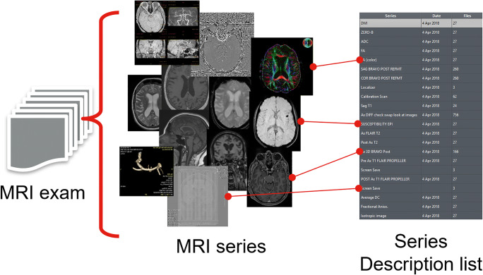
The “Series Description” (SD) attribute (0008,103E) is a short piece of text describing the series. It is an optional DICOM attribute that is nevertheless used widely in DICOM viewers to identify series. When loading an exam, the user (e.g., a radiologist) usually is provided with a list containing the series available in the exam and their descriptions, in order to open the series in which he or she is interested (Fig. 1). However, the SD is free text that can suffer from very high variability:

• It depends on the manufacturers.

• It can be modified by the radiology professionals.

• It can also be related to specific in-house protocols.

Fig. 1.

Content of an MRI exam (left) and examples of the variability of the series descriptions (right)

To add to this variability, the SD also mixes information of very different nature. It can combine information about the contrast, the image orientation, the postprocessing, and more. In Fig. 1 (left), we show a few different examples highlighting the diversity of information an MRI study contains. At our institution, we could identify hundreds of thousands of unique brain MRI SD in the last years. In these conditions, it appears challenging to rely only on simple SD mappings to properly identify imaging series of interest.

In everyday practice, even the radiologists may suffer from the inconsistency of the SD. Sometimes they may have to open several series before finding the one they want. In “Data Annotation Process,” we show that more than 10% of SDs do not allow the radiologist to identify the sequence type. Having a more standardized SD may also help to define hanging protocols (i.e., a way of automating the ordering of image series being displayed on the screen).

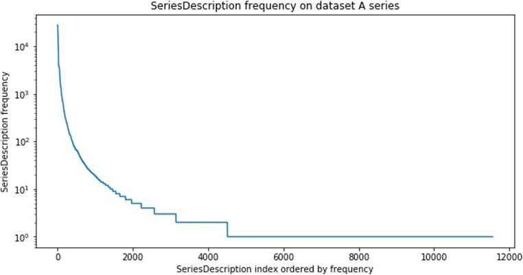
SDs are thus not always reliable enough to be used for image categorization. However, the SD can still hold valuable information about the series. We assume in this work that it can be used to assist the manual labeling of our data. Indeed, even if they are highly variable, a few unique SDs are often commonly used for specific contrasts (e.g., “T1 AXIAL POST” is commonly used to describe a postcontrast T1-weighted axial sequence). Looking at the distribution of the unique occurrences of the SD in our datasets highlighted that a few hundred unique SD could identify a large percentage of our datasets (see Fig. 2). In “Method: Finding Relevant Features and Building a Classifier,” we show how we use the SD to leverage the annotation process (and make it fast and easy).

Fig. 2.

Unique series descriptions (SD) frequency over all series of dataset A. Logarithmic scale

Material and Method

To develop and test the proposed solution, we focused on brain MRI images. MRI is among the modalities with the most sequences in a single study, especially in brain imaging. Thus, we believe that if our method works for this challenging use case, our solution could be generalizable to less diverse modalities and anatomies. We categorized the series into eight different classes (T1, T2, fluid attenuation inversion recovery (FLAIR), diffusion, susceptibility and gradient echo, angiography, localizer, and others), covering the most common contrast acquisitions for brain MRI.

To train, validate and test our approach, we used two different brain MRI datasets:

• Dataset A: one large dataset from our institution (used for first training, validation and testing).

• Dataset B: one large dataset from another institution with several different outpatient clinics outside the USA.

Our approach is designed to fulfill the following criteria:

1. Be easily reproducible and sufficiently generic to be extended to other anatomies and modalities

2. Be scalable (very fast inference time to facilitate integration in the clinical workflow and cost-effective)

3. Have low generalization error (to be able to be used on data from other institutions):

   1. on old studies (for cohort creation);
   2. on recent studies with new machines (for deployment).

4. Provide confidence scores of each prediction to request manual inspection if needed

Material

Data Inventory

In this work, we use brain MRI acquisitions from two different datasets originating from different places:

• Dataset A: 32,844 studies acquired between 2007 and 2017 (see Fig. 3 for distribution across years) from hospital A in our institution (the decrease in the number of cases after 2012 is due to the methodology used for the cohort selection of our dataset, which was based on exam codes more commonly used before 2012, reflecting the changes of protocols over time).

• Dataset B: 6325 studies acquired in 2017, from 39 different clinical sites.

Fig. 3.

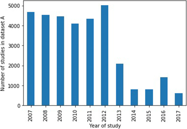
Distribution of year of study for dataset A

Note that these two datasets contain the full MRI studies, as they are used in a radiology environment. Dataset A is our working dataset. It is used for training, validation, and the first tests of our hypothesis. To this purpose, it has been split randomly into training (70%), validation (10%), and testing (20%) sets at the exam/study level. Dataset B is used to validate the generalization of our classification model trained on dataset A (it is never used for training).

In Table 1, we list the number of studies and series included in each dataset. In Table 2, we show the number of studies from different manufacturers in each dataset.

Table 1.

Dataset descriptions and figures

	No. of studies	No. of series	No. of annotated series
Dataset A	32,844	707,040	600,069
- Training	22,850	491,822	471,329
- Validation	3430	74,091	62,871
- Testing	6564	141,127	119,869
Dataset B	6765	86,513	69,356

Table 2.

Number of studies per manufacturer for each dataset

	GE Healthcare	Siemens	Toshiba	Philips
Dataset A	20,171	12,594	79	0
Dataset B	6281	104	277	103

Despite the fact that all studies are brain MRI, they have been collected in different patient settings. Dataset A has been collected with a few selection criteria: the presence of four defined sequences (T1-weighted pre- and postcontrast, FLAIR and ADC) and the manufacturer attribute (0008,0070) had to be specified in the DICOM file (to allow for data analysis; it is also a required attribute). Dataset B was collected consecutively and contained at least four sequences.

Data Annotation Process

The series of each dataset are labeled into 8 different categories as follows:

• T1-weighted (labeled t1)

• T2-weighted (labeled t2)

• Fluid attenuation inversion recovery (labeled flair)

• Diffusion (labeled diffusion)

• Susceptibility-weighted and gradient echo (labeled suscgre)

• MR angiography (labeled mra)

• Localizers used for planning (labeled scout)

• Screenshots, perfusion, spectroscopy… (labeled other)

It is important to mention that these categories cover most of the possible series types that can be found in an MRI study of the brain.

It would be very time-consuming to label each series by visual inspection. Thus, we leverage the SD attribute of the series to annotate the data more efficiently.

The annotation process consists of the following steps:

1. The SD attribute of each series is extracted.

2. The most common SDs are selected for annotation (such as to cover approximately 80% of the series in the dataset).

3. The selected SDs are labeled by a radiologist as one of the abovementioned 8 categories or to “unknown” if it is not possible to decide (i.e., the SD “T1 AXIAL POST” is labeled as t1, but the SD “REFORMAT” is labeled as unknown because it is impossible to know what type of contrast it is just based on the SD content).

4. For the series labeled as unknown, there are two possible options:

   1. If the SD is explicit (contains meaningful contrast or sequence information): the radiologist is presented with 5 random examples of images corresponding to this SD. Then, either the radiologist can decide on the label, or if it is not possible to decide, the SD remains labeled as unknown;
   2. If the SD is not explicit (for instance “Axial” or “REFORMAT”), the SD remains labeled as unknown.

In Table 3, we show for each dataset the number of unique SDs they contain, how many SDs were labeled and to how many labeled series the SD correspond to. We notice that by labeling approximately 10% of the unique series descriptions, approximately 80–85% of the related series can be labeled.

Table 3.

Number of labeled SDs per dataset

	No. of unique SDs	No. of unique labeled SDs	No. of labeled series (not labeled as “unknown”) (% of series)
Dataset A	11,558	1023	600,069 (87%)
Dataset B	2753	328 (43 “unknown”)	67,958 (79%)

For dataset B, we annotated the 238 most frequent SDs and added 90 other SDs for series from under-represented manufacturers (see Table 2 for the distribution). Over the 328 SDs labeled for this dataset, more than 10% were labeled as “unknown.”

In “Series Description Variability Analysis,” we show the figures corresponding to the SD overlap across datasets.

Method: Finding Relevant Features and Building a Classifier

In this section, we present the two main steps of the classifier construction. First, a few discriminating DICOM attributes are selected (to keep the classifier as simple as possible and to obtain a classification that is easily interpretable). Second, a training validation process is performed. This section essentially aims to explain and justify our choices. The results are presented in the following section.

Features Selection and Extraction

Instead of retaining all possible DICOM attributes, we begin with a simple and reasonable selection. We preselect the DICOM attributes coming from the following modules:

• The MR Image module: 51 attributes (type 1: 8, type 2: 7)

• The Enhanced MR Pulse Sequence Module: 18 attributes (all type 1)

• The Image Pixel module (corresponding to the image pixel data characteristics): 23 attributes (type 1: 19, some are redundant with the MR image module)

• Contrast/bolus module: 1 attribute (type 2).

These DICOM attributes are extracted by scanning each series of our datasets. We use the Python package Pydicom [36] for reading the DICOM metadata and a MongoDB database [37] to store these values.

A first filtering is applied on these attributes just by checking if they have more than one unique value over the training set (including the possibility of not being specified). Otherwise, this attribute is considered as not relevant, as it has the same value across all classes.

Then, the attributes are tokenized (using one hot encoding). There are several types of attribute values that we transform in the following way:

• Number: converted to float by default

• String: converted to binary features as follows:

  • If the standard defines a finite set of predefined values, each possible value of the standard is considered as a binary feature.
  • If there are no predefined values, the training dataset is used to identify the possible values, and these are converted into binary features.

• List of strings: each value of the list is converted into a binary feature (following the same procedure described above).

• Exceptions: for the attribute “Pixel Spacing” (0028,0030), only the first floating value is retained as pixels in slices are generally isotropic.

For instance, the attribute “Photometric Interpretation” (0028,0004) can have the values “MONOCHROME1,” “MONOCHROME2,” “RGB”… We will thus consider a feature RGB that will take binary values. This also means that if the feature RGB is set to 1, the feature MONOCHROME1 will be necessarily set to 0.

We add one feature that is not directly derived from a DICOM attribute: the number of image instances per series by identifying the number of files that have the same Series Instance UID (0020,000E). This is easily computed when parsing all DICOM files.

Classifier Training

Once the features are tokenized and selected, we are ready to train the classifier. The training process follows classical machine learning rules:

• Training, validation, and testing datasets are defined (the testing set being used in the final stage after classifier and hyperparameters selection).

• For each trained classifier, a grid-search is applied to find the best hyperparameters.

• The selection of the hyperparameters search is done by relying on the model results on the validation set.

In this work, we use a random forest classifier [38], as it has proved to have a very good bias and variance trade-off and is very robust to overfitting (due to the bootstrap training of each single tree). This classifier also allows us to derive confidence scores that are very important to provide certainty information on the results to the end user. This classifier is also very fast to train and test, one of the requirements of the solution we want to build. This also allows more flexibility and does not require any expensive GPU resources (as is currently the trend).

Note on the Anatomical Plane Information

The anatomical plane information (sagittal, coronal, axial) is very often specified in the SD (see the examples in Fig. 1). However, this information can be easily derived from the Image Orientation Patient (0020,0037) DICOM attribute. This attribute gives the direction cosines of the first row (first three values) and first column (last three values) of an image with respect to the patient. The anatomical plane information can then be computed by finding the main direction of the normal to the slices.

Therefore, relying directly on the aforementioned attribute is much more reliable than using information entered manually in the series description.

Technical Details

The development of each step of this work is performed using Python open-source packages:

• Pydicom [36] for DICOM metadata extraction.

• MongoDB [37] for the data storage and organization.

• Pandas [39] for the data manipulation and filtering.

• Scikit-learn [40] for the machine learning part (classifier training and results analysis).

All steps are performed on a standard laptop CPU with a reasonable amount of RAM. Once the DICOM metadata is retrieved, the preprocessing steps do not take more than a minute to complete (on the full training dataset); the classifier training takes seconds.

Results and Discussion

In this section, we present quantitative results for each part of the process. We first provide a few figures describing the SD population (“Series Description Variability Analysis”). We then show the intermediary steps of the feature extraction procedure (“Across Institutions”). Finally, we present the classification results for each of the datasets (“Classification”).

Series Description Variability Analysis

Across Time

We split dataset A into two chunks of approximately the same size: series acquired before 2010 and series acquired after 2010. These datasets contain 3520 and 8949 unique SDs, respectively. The size of the unique SD intersection is 921 SDs.

For instance, after 2010, new SDs have been introduced, such as “Dif,” “Dif_FA,” “Dif_ADC,” or “Ax 3D SWAN.” New SDs can be introduced for several different reasons: acquisitions from a different scanner/model/software, introduction of new sequences, and/or protocol changes.

Across Institutions

Datasets A and B contain 11,558 and 2753 unique SDs, respectively. Datasets A and B have only 134 unique SDs in common. This small SD overlap reinforces the observation that relying on SD mapping lists alone is not generalizable at all.

Feature Extraction

For the feature extraction validation, we use dataset A. Starting from 73 DICOM attributes (see the Appendix for the full list), we apply the steps described in “Method: Finding Relevant Features and Building a Classifier.” The results after each step are given in Table 4. The final list of DICOM attributes and the values tokenized as features are given in Table 5.

Table 4.

Number of DICOM attributes remaining after each selection and processing step

	Number of DICOM attributes
Initial state	73
Keeping type 1 and type 2 DICOM attributes	35
Meaningless attributes removal	17
	Number of features
Attributes tokenization to features	30

Table 5.

Final list of DICOM attributes kept for the classification task

DICOM attribute	DICOM tag	DICOM values tokenized as features
Echo time	(0018,0081)
Inversion time	(0018,0082)
Echo train length	(0018,0091)
Repetition time	(0018,0080)
Trigger time	(0018,1060)
Sequence variant	(0018,0021)	SK, MTC, SS, TRSS, SP, MP, OSP, TOF, NONE
Scan options	(0018,0022)	PER, RG, CG, PPG, FC, PFF, PFP, SP, FS
Scanning sequence	(0018,0020)	SE, IR, GR, EP, RM
MR acquisition type	(0018,0023)	2D, 3D
Image type	(0008,0008)	ORIGINAL, DERIVED, PRIMARY, SECONDARY
Pixel spacing	(0028,0030)
Slice thickness	(0018,0050)
Photometric interpretation	(0028,0100)	RGB, MONOCHROME1, MONOCHROME2
Number of images
Contrast bolus agent	(0018,0010)

Classification

In this section, we present the quantitative results on datasets A and B. The classifier is trained on the training set of dataset A and is then used on all other datasets without retraining. This allows us to validate the robustness and generalization capability of our approach.

Dataset A

Hyperparameter Search and Best Classifier Selection

We did not set a maximum tree depth, but we tuned the minimum leaf size (ranging from 5 to 50). The classes are balanced to have the same weight while training. We also compared the results on the validation set for the following parameters: split criterion (Gini vs entropy) and number of trees (from 1 to 200).

The best classification results were obtained with the random forest classifier with minimum leaf size of 10, entropy split criterion, and 150 trees. We use this classifier for all subsequent experiments.

Evaluating the Robustness Across Time

In this experiment, we want to assess whether our approach is robust across time. To test this hypothesis, we isolate the studies performed in 2017 (14,410 series) from the remainder of the dataset, and we use it as our test set. This set is called A₂₀₁₇. We then build 10 datasets A_N, where N is in ⟦2008, 2016⟧ and where A_N holds studies acquired before year N. Each dataset A_N is split into training and validation sets (80%, 20% respectively).

To train the random forest on these datasets, we keep the parameters that were selected in the previous hyperparameter search. The performance of the trained random forest is then evaluated on the series acquired in 2017.

Figure 4 shows the accuracy on the testing dataset A₂₀₁₇ when training the classifier on datasets A_N. The percentage of predictions with confidence scores below 0.5 is also given. It reflects the uncertainty of the predictions. We observe that by continuing to add more recent studies to the training set, the uncertainty of the predictions decreases, and the accuracy also increases. In particular, we can see that after adding data from 2011, the accuracy becomes very high and remains very high.

Fig. 4.

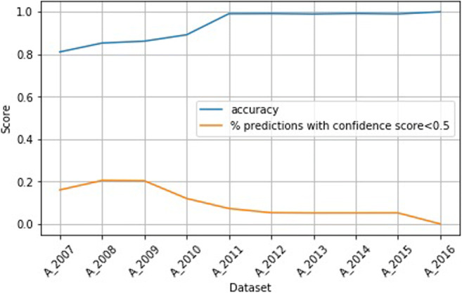
Accuracy and uncertainty on dataset A₂₀₁₇ when training on datasets A_N

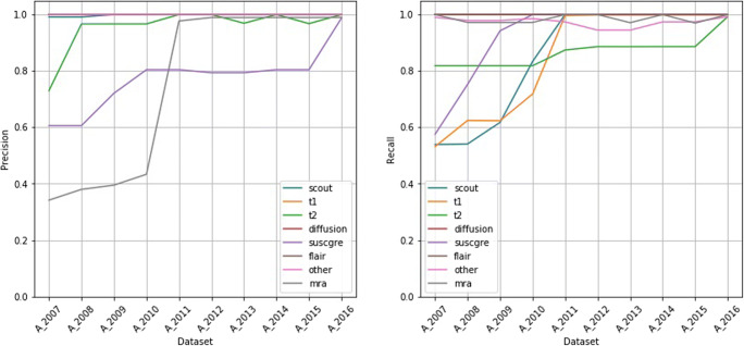
Figure 5 shows the precision and recall per sequence type on dataset A₂₀₁₇ when training the classifier on datasets A_N. For the classes diffusion, flair, and other, we see very high precision and recall across training sets. For the classes mra and suscgre, the recall is very high, while the precision improves when adding more recent data. In contrast, for the classes t1, t2, and scout, the precision is very high, while the recall improves when adding more recent data.

Fig. 5.

Precision and recall per sequence type on dataset A₂₀₁₇ when training on datasets A_N

Results on the Full Dataset

The following results are obtained on the full testing set of dataset A (119,869 series) with the random forest classifier trained on the training set of dataset A (417,329 series).

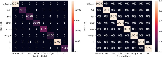
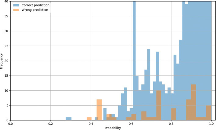
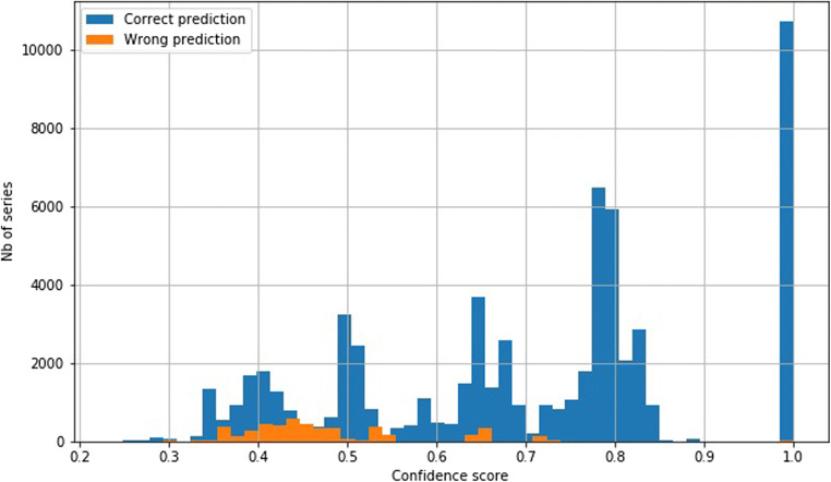
The overall error rate is 0.05% (59 errors). Figure 6 shows the confidence matrices of the absolute and the relative results per class. The y-axes show the true label, while the x-axes correspond to the predicted classes. For instance, all diffusion series are classified as diffusion (first row of the confidence matrices). The areas under the ROC curves (AUC) are 100.0, 99.99, 99.99, 99.99, 99.99, 100.0, 99.99, and 99.99 for the classes diffusion, flair, mra, other, scout, suscgre, t1, and t2, respectively. Figure 7 shows the probability distributions for the correct and incorrect predictions.

Fig. 6.

Absolute and relative confusion matrices on all series of dataset A, with predictions from the highest scores

Fig. 7.

Confidence scores distribution for dataset A for correct (blue) and incorrect (orange) predictions. The y-axis range has been reduced to show the distribution of incorrect predictions (the frequency of the correct predictions extends well beyond 40)

Errors Analysis

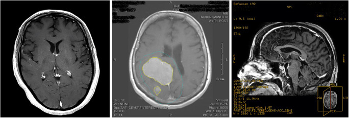
As mentioned earlier, the results for the test set of dataset A are very high. However, there are a few errors (59 in total), as shown in Fig. 6. We analyzed the erroneous predictions that have confidence scores above 0.5 (49 predictions, as shown in Fig. 7) by opening the corresponding series in a DICOM viewer and by checking the true and predicted labels. For 32 cases (~ 65%), the second-most probable prediction was correct. We discovered that 30 series (61%) were incorrectly annotated and correctly classified, 8 series (16%) had ambiguous annotations, 7 series (14%) were incorrectly classified but the prediction was partially true (see below explanations), and the remaining 4 series (8%) were simply incorrectly classified with low confidence scores. Figure 8 shows three examples of incorrectly annotated series. We noticed that most of the time, this occurs when a derived series, such as a maximum intensity projection (MIP) or a screenshot, is saved using the SD of the original series. Interestingly, we observed that the original series were always correctly classified. As our annotation process is based on the SD (see “Data Annotation Process”), this type of error may sometimes occur. Some cases were more ambiguous; for example, four series corresponding to MIP series were generated from susceptibility images. Those series were annotated as mra (which may be arguable because of the high prevalence of MIP series derived for angiogram studies in the datasets) and classified as suscgre. For other series, some predictions were false but not that far from the truth. The four series incorrectly classified all correspond to a confusion between the classes t1, mra, and other.

Fig. 8.

Left: series annotated as t2 (SD: “Ax T2 POST”), correctly classified as t1. Middle: series annotated as t1 (SD: “Ax T1 POST”) and classified as other. Right: series annotated as t1 (SD: “SAG BRAVO POST RFMT”) which is a screenshot of a t1 series

Dataset B

Results

Table 6 shows the results for dataset B. When considering the predicted class with the highest confidence score, the overall accuracy is 93.0%, while when taking into account only the predictions with confidence score above 0.5, the accuracy reaches 97.4%. The accuracy is also given per manufacturer. The best results are obtained for manufacturers 1 and 2, ranging from 99 to 100% (which is not very surprising considering that the classifier has been trained with data only from these manufacturers).

Table 6.

Accuracy results for dataset B, on all series and per manufacturer

	Percent of series set as “unknown” (number)	Accuracy (%)
Best class result	0 (0)	93.0
Best class with confidence score > 0.5	23.4 (15,900)	97.4
Per Manufacturer (best class with confidence score > 0.5)
- GE Healthcare	23.5	99.0
- Siemens	4.7	100.0
- Toshiba	19.6	72.5
- Philips	43.2	71.6

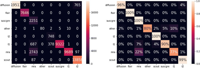
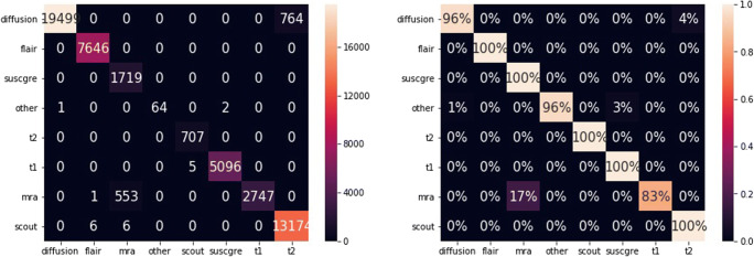
Figures 9 and 10 show the absolute and relative confidence matrices given the best predicted class for all series and for all series with confidence scores above 0.5 respectively.

Fig. 9.

Absolute and relative confusion matrices on all series of dataset B, with predictions from highest scores

Fig. 10.

Absolute and relative confusion matrices on all series with confidence scores above 0.5 of dataset B, with predictions from highest scores

Figure 11 shows the confidence scores distribution over all of the series for correct and incorrect predictions. A few incorrect predictions have confidence scores of 1.0. For all of these series, we observed that the ImageType tag was incorrectly populated with values corresponding to T2-weighted series.

Fig. 11.

Confidence scores distribution for dataset B for correct (blue) and incorrect (orange) predictions

Errors Analysis

Similar to dataset A, we performed a deep analysis on the errors. We observed that the incorrect predictions with high confidence scores (> 0.75) were all due to false or very ambiguous annotations. This corresponds to 48 cases, from which 2 cases were labeled as t2 (the SD was “COR T2 HIPOCAMPO”), but after opening those images, we discovered that they were flair images. The remaining 40 cases were B0 diffusion maps predicted as t2, which is relevant as B0 diffusion maps are T2-weighted. There were also 1290 incorrect predictions with low confidence scores (< 0.75 and > 0.5). Of those cases, 722 (56%) diffusion series were predicted as t2 (an example is given in Table 7). This is explained by the fact that the acquisition parameters used correspond to t2 series, and the ImageType attribute was not correctly filled by the manufacturers Siemens and Philips (it was set to [ORIGINAL, PRIMARY], although it should be [ORIGINAL, DERIVED], as the diffusion maps are derived maps). For 553 cases (43%), postcontrast T1-weighted series reformatted as 3D were predicted as t1, which makes some sense. We found 6 cases (0.5%) with incorrect labels (e.g., a series with description “SAG T1 FAT POS” was a flair series and was predicted as such). The remaining 9 cases (0.7%) were false predictions with very low confidence scores (close to 0.5) and corresponded to rare sequences in our training set (e.g., perfusion series).

Table 7.

Example of a study with bad prediction results (study from the manufacturer Philips)

Series description	anatomical_plane	seqfamily_manual_label	seqfamily_pred	seqfamily_pred_proba
SAG T1 TFE POS GD	Sagittal	t1	mra	0.424657
SAG FLAIR	Sagittal	Flair	Flair	0.694975
rSAG T1_SE	Sagittal	t1	t1	0.578059
sReg-rDIFUSAD SENSE b1000	Axial	Diffusion	t2	0.719391
SAG T2 FLAIR 3D ISO	Sagittal	NaN	Flair	0.723593
SWlp Filme	Axial	suscgre	mra	0.451012
COR T1 3D TFE ISO POS GD	coronal	t1	mra	0.460067
rDIFUSAO EPI	Axial	Diffusion	t2	0.716603
rSAG T1_SE	Sagittal	t1	t1	0.578059
sReg-rDIFUSAO SENSE b0	Axial	Diffusion	t2	0.719391
SAG T2 3D DRIVE	Sagittal	NaN	t2	0.632825
AXI T2 MVXD	Axial	t2	t2	0.825407
SAG T2 3D DRIVE	Sagittal	NaN	t2	0.632825
AXI FLAIR	Axial	Flair	Flair	0.694975
SWIp HR	Axial	suscgre	mra	0.370486
rSWIp	Axial	suscgre	mra	0.447397
COR T2 MVXD	Coronal	t2	t2	0.832831
Reg-rDIFUSAO SENSE	Axail	Diffusion	t2	0.716603
AXI T1 TFE POS GD	Axial	t1	mra	0.424657
rSAG T1 3D TFE ISO POS GD	Sagittal t1	t1	t2	0.381115
dReg-rDIFUSAO SENSE MAPA ADC	Axial	Diffusion	Diffusion	1.000000

Study Level Analysis

Tables 7 and 8 show examples of predictions for all series of two complete studies. Those examples show the variety of SDs that can be found in two different studies (we also notice that the series descriptions combine English and Portuguese words), and they also show the anatomical plane results (see “Note on the Anatomical Plane Information”) and the confidence scores for all prediction results.

Table 8.

Example of a study with good prediction results (study from the manufacturer GE Healthcare) (NaN means that the series has not been manually labeled)

Series description	anatomical_plane	seqfamily_manual_label	seqfamily_pred	seqfamily_pred_proba
Apparent diffusion coefficient (mm2/s)	Axial	Diffusion	Diffusion	1.000000
FILT_PHA: 3D SWAN T2*	Axial	suscgre	suscgre	0.502039
MPRO Ob_Cor_A-> P_Average_sp:3.0_th:3.0	Coronal	Unknown	mra	0.396210
Ph1/MASC E ANGIO VENOSA	Unknown	mra	mra	0.448613
Ax T2 FLAIR	Axial	Flair	Flair	0.783323
ANGIO ARTIRIAL 3DTOF	Axial	mra	mra	0.611182
RECON ARTERIAL	Unknown	NaN	mra	0.650378
RECON VENOSA	Unknown	NaN	mra	0.426741
Sag T1	Sagittal	t1	t1	0.385957
SAG 3D FAT POS	Sagittal	Unknown	mra	0.431439
MASC E ANGIO VENOSA	Unknown	mra	mra	0.448613
3D SWAN T2*	Axial	suscgre	suscgre	0.502039
MASC E ANGIO VENOSA	Unknown	mra	mra	0.448613
MPR Ob_Sag_L-> R_Average_sp:7.0_th:7.0	Sagittal	Unknown	scout	0.364711
RECON VENOSA	Unknown	NaN	mra	0.462741
Ax FSE T2 FAT	Axial	t2	t2	0.789516
MPR Ob_Ax_S-> I_Average_sp:3.0_th:3.0	Axial	Unknown	mra	0.39210
(3526/1201/1)-(3526/1200/1)	Unknown	NaN	mra	0.507088
PU:AX DIFUSAO	Axial	Diffusion	Diffusion	0.673117
RECON ARTERIAL	Unkown	NaN	mra	0.651717
AX DUFISAO	Axial	Diffusion	Diffusion	0.637458
RECON ARTERIAL	Unknown	NaN	mra	0.650378
PJN:ANGIO ARTERIAL 3DTOF	Unknown	mra	mra	0.845646
COR FSE T2 FT	Coronal	t2	t2	0.796161
Exponential apparent diffusion coefficient	Axial	Diffusion	Diffusion	1.000000

The results can also be analyzed at the study level instead of at the series level. For each study, we can keep for each class one series that has been labeled as such with the highest score (meaning we would have one series for each class of each study). We can then compute the accuracy on those series. The accuracies for flair, mra, and scout are all 100%. The accuracies reach 98.7% for t2, 94.4% for diffusion, 89.4% for t1, and 87.1% for suscgre.

Computation Time

During the experiments, we also evaluated the performance of the solution. While the classification time per series is almost instantaneous, the overhead comes from the series metadata reading. Once the metadata are extracted from the DICOM file, it takes 0.4 ms per series for the features processing and prediction (on a laptop with a dual-core Intel Xeon CPU E3-1505M 3GHz). It is worth mentioning that this process could be easily parallelized to achieve even faster computation.

Discussion

The results presented above allow us to answer several questions and to more thoroughly understand the advantages and limits of our approach.

The study on SD variability across time and institutions (“Series Description Variability Analysis”) validates our approach and clearly invalidates the SD lookup table approach. The number of unique SDs used can change greatly across time and location. Creating and maintaining a mapping list would be very time-consuming and not sufficiently reliable. Indeed, we have found that more than 10% of SDs are not informative enough for the radiologist.

The first experiment on dataset A with training datasets containing relatively recent studies shows the robustness of the method (see “Evaluating the Robustness Across Time”). Using older training data than the testing data is not a problem. The classifier remains very robust even when the testing data are a few years more recent than the training data. This gives us good reason to think that we would not have to retrain a new classifier too frequently. The slight changes that we may observe are most likely related to changes on the manufacturer side and in clinical practice (such as new protocols). The uncertainty given by the algorithm also provides good clues to what data to add in the training set to enhance the results.

The experiments on the full dataset A show the maximum reachable accuracy when working on a dataset similar to the training set. The accuracy achieved is almost perfect, with an error rate of 0.05% (see “Results on the Full Dataset”). The trained classifier can thus be used with high confidence for cohort creation and as a component for series selection to automate inputs to algorithm routing. The error analysis (see “Errors Analysis”) shows that approximately 60% of the errors were actually due to incorrect annotations, and for all of those cases, the predictions were effectively correct. Other errors were due to the ambiguity of the annotations. However, the predictions were very close to the true labels. Only 8% of the errors were real errors (but could be explained by the lack of relevant DICOM attributes), and all occurred due to confusion between the classes t1, mra, and other.

The experiments on dataset B show how the classifier can generalize to other types of datasets, coming from other institutions, from other manufacturers and from other countries. For data from manufacturers GE Healthcare and Siemens that were represented in dataset A, the classifier generalizes very well (almost perfectly) for diffusion, flair, suscgre, and t2 series (between 99 and 100% accuracies). When testing on the two other manufacturers, Toshiba and Philips, the overall accuracy decreases for two main reasons: (1) confusion between diffusion and t2 classes due to the incorrect usage of the DICOM attribute ImageType and (2) contrasted T1 series (labeled as t1) classified as mra. Adding the recent DICOM attribute “diffusion B-value” (type 1 tag) as a feature would help resolve a large number of these wrong predictions. The error analysis also shows that incorrect predictions with high confidence scores were all due to incorrect or ambiguous annotations, meaning that the confidence score is very reliable for filtering the predictions.

Although we took all of the precautions to build our approach on DICOM attributes required by the DICOM standard (which were supposedly consistent across vendors), the results show that inconsistencies remain across vendors. Even required attributes can be incorrectly populated and can lead to confusion.

The computation time of this approach (0.4 ms per series) is a considerable advantage when compared to image-based approaches. The overhead of such an approach lies at the DICOM content reading level and not at the inference level (however, this is an incompressible computation time, whatever the chosen solution).

Conclusion

In this work, we presented an approach to automatically classify series of brain MRI studies into 8 different categories covering the most common sequence types. The solution presented relies on DICOM metadata only, including acquisition parameters and image-related information. The approach relies on DICOM attributes that are required by the standard, thus ensuring the best generalization capability.

A specific strategy has been employed to rapidly and efficiently label the datasets based on series descriptions, allowing us to test our solution on two different large and diverse datasets (hundreds of thousands of series). These datasets cover almost all of the use cases that could be found in a real deployment environment (different institutions, manufacturers, countries) and thus gives us very high confidence in the presented results. The approach generalizes well across time, and a few years’ difference between the training and testing sets does not overly degrade the results. The method proposed also generalizes very well to datasets from different institutions, reaching an accuracy of 97.4% on predictions with confidence scores above 0.5. The main differences in performance are observed when testing data from different manufacturers that were not represented in the training set (Toshiba and Philips). An analysis of the errors shows that DICOM metadata population deviating from the standard could not be captured by our classifier and that some classes can sometimes be ambiguous (t1, mra and other). Should a screenshot of a contrasted T1-weighted series be labeled as a t1 or other (i.e., “screenshot”)? However, we believe that this ambiguity would depend on the use case. The confidence scores for each class thus provide valuable information that could be further used for different scenarios of usage.

For future improvements, we would like to add more classes to refine the class other. This class contains very different sequence types (perfusion, spectroscopy, screenshots…) that were not well represented in the training dataset and that should be considered as new classes in the next experiments.

The methodology presented is sufficiently generic to be adapted to changes and the evolution of the DICOM standard. New DICOM attributes can be easily added for training (for instance, the “Diffusion B-value” attribute) in future versions. However, this supposes that the manufacturers follow the established standard.

We hope that in the future, both medical imaging institutions and manufacturers can work on the standardization of the naming of MRI sequences. While waiting for this progress to occur, the solution proposed shows that leveraging the DICOM metadata can be relevant for the categorization of the most common MRI sequence types. To introduce more granularity, relying on the pixel data may have to be examined.

In any case, this solution is already a good start for the selection of some types of sequences, even on datasets coming from different institutions. It can be used as a first filtering step to prevent encountering image-based inference in all series.

Appendix A

The original list of DICOM attributes was the following:

Image Type, Samples Per Pixel, Photometric Interpretation, Bits Allocated, Bits Stored, High Bit, Scanning Sequence, Sequence Variant, Scan Options, MR Acquisition Type, Repetition Time, Echo Time, Echo Train Length, Inversion Time, Trigger Time, Sequence Name, Angio Flag, Number Of Averages, Imaging Frequency, Imaged Nucleus, Echo Number, Magnetic Field Strength, Spacing Between Slices, Number Of Phase Encoding Steps, Percent Sampling, Percent Phase Field Of View, Pixel Bandwidth, Nominal Interval, Beat Refection Flag, Low RR Value, High RR Value, Intervals Acquired, Intervals Rejected, PVC Rejection, Skip Beats, Heart Rate, Cardiac Number Of Images, Trigger Window, Rate, Reconstruction Diameter, Receive Coil Name, Transmit Coil Name, Acquisition Matrix, In Plane Phase Encoding Direction, Flip Angle, SAR, Variable Flip Angle Flag, DB-Dt, Temporal Position Identifier, Number Of Temporal Positions,Temporal Resolution, Pulse Sequence Name, MR Acquisition Type, Echo Pulse Sequence, Multiple Sin Echo, Multiplanar Excitation, Phase Contrast, Time Of Flight Contrast, Arterial Spin Labeling Contrast, Steady State Pulse Sequence, Echo Planar Pulse Sequence, Saturation Recovery, Spectrally Selected Suppression, Oversampling Phase, Geometry Of K Sapce Traversal, Rectilinear Phase Encode Reordering, Segmented K Space Traversal, Coverage Of K Space, Number Of K Space Trajectories, Pixel Spacing, Slice Thickness, Images In Acquisition, Contrast Bolus Agent.

References

- 1.Choy G, Khalilzadeh O, Michalski M, Do S, Samir AE, Pianykh OS, Geis JR, Pandharipande PV, Brink JA, Dreyer KJ. Current applications and future impact of machine learning in radiology. Radiology. 2018;288(2):318–328. doi: 10.1148/radiol.2018171820. [DOI] [PMC free article] [PubMed] [Google Scholar]
- 2.Koohy H. The Rise and Fall of Machine Learning Methods in Biomedical Research. F1000Research. 2018;6:2012. doi: 10.12688/f1000research.13016.2. [DOI] [PMC free article] [PubMed] [Google Scholar]
- 3.Jiang F, Jiang Y, Zhi H, Dong Y, Li H, Ma S, Wang Y, Dong Q, Shen H, Wang Y. Artificial intelligence in healthcare: past, present and future. Stroke and Vascular Neurology. 2017;2(4):230–243. doi: 10.1136/svn-2017-000101. [DOI] [PMC free article] [PubMed] [Google Scholar]
- 4.Allen Bibb, Seltzer Steven E., Langlotz Curtis P., Dreyer Keith P., Summers Ronald M., Petrick Nicholas, Marinac-Dabic Danica, Cruz Marisa, Alkasab Tarik K., Hanisch Robert J., Nilsen Wendy J., Burleson Judy, Lyman Kevin, Kandarpa Krishna. A Road Map for Translational Research on Artificial Intelligence in Medical Imaging: From the 2018 National Institutes of Health/RSNA/ACR/The Academy Workshop. Journal of the American College of Radiology. 2019;16(9):1179–1189. doi: 10.1016/j.jacr.2019.04.014. [DOI] [PubMed] [Google Scholar]
- 5.DICOM standard. [Online]. Available: https://www.dicomstandard.org/. [Accessed: 20-Sep-2018].
- 6.Petrakis EGM, Faloutsos A. Similarity searching in medical image databases. IEEE Trans Knowl Data Eng. 1997;9(3):435–447. doi: 10.1109/69.599932. [DOI] [Google Scholar]
- 7.Lehmann TM, Schubert H, Keysers D, Kohnen M, Wein BB: The IRMA Code for Unique Classification of Medical Images, presented at the Medical Imaging. San Diego 2003, p 440
- 8.M. O. Gueld et al., Quality of DICOM Header Information for Image Categorization, presented at the Medical Imaging 2002, San Diego 280–287.
- 9.Bergamasco LCC, Nunes FLS. Intelligent retrieval and classification in three-dimensional biomedical images — a systematic mapping. Comput Sci Rev. 2019;31:19–38. doi: 10.1016/j.cosrev.2018.10.003. [DOI] [Google Scholar]
- 10.Kwak D-M, Kim B-S, Yoon O-K, Park C-H, Won J-U, Park K-H. Content-based ultrasound image retrieval using a coarse to fine approach. Ann NY Acad Sci. 2002;980(1):212–224. doi: 10.1111/j.1749-6632.2002.tb04898.x. [DOI] [PubMed] [Google Scholar]
- 11.Anavi Y, Kogan I, Gelbart E, Geva O, Greenspan H: Visualizing and Enhancing a Deep Learning Framework Using Patients Age and Gender for Chest X-ray Image Retrieval, presented at the SPIE Medical Imaging, San Diego 2016, p 978510
- 12.Stanley RJ, De S, Demner-Fushman D, Antani S, Thoma GR. An image feature-based approach to automatically find images for application to clinical decision support. Computerized Medical Imaging and Graphics. 2011;35(5):365–372. doi: 10.1016/j.compmedimag.2010.11.008. [DOI] [PMC free article] [PubMed] [Google Scholar]
- 13.Quellec G, Lamard M, Cazuguel G, Roux C, Cochener B. Case retrieval in medical databases by fusing heterogeneous information. IEEE Trans Med Imaging. 2011;30(1):108–118. doi: 10.1109/TMI.2010.2063711. [DOI] [PubMed] [Google Scholar]
- 14.de Herrera AGS, Schaer R, Bromuri S, Muller H: Overview of the ImageCLEF 2016 medical task, in Working Notes of CLEF 2016 (Cross Language Evaluation Forum), 2016.
- 15.de Herrera AGS, Markonis D, Müller H. Bag-of-colors for biomedical document image classification. In: Greenspan H, Müller H, Syeda-Mahmood T, editors. Medical Content-Based Retrieval for Clinical Decision Support. Berlin: Springer Berlin Heidelberg; 2013. pp. 110–121. [Google Scholar]
- 16.Cirujeda P, Binefa X: Medical Image Classification via 2D Color Feature Based Covariance Descriptors, Proceedings of the Working Notes of CLEF, Toulouse, France, 8–11 September 2015, 2015, p. 10
- 17.Pelka O, Friedrich CM: FHDO Biomedical Computer Science Group at Medical Classification Task of Image CLEF 2015, Proceedings of the Working Notes of CLEF, Toulouse, France, 8–11 September 2015, 2015, p. 15
- 18.Kumar A, Kim J, Lyndon D, Fulham M, Feng D. An ensemble of fine-tuned convolutional neural networks for medical image classification. IEEE J Biomed Health Inf. 2017;21(1):31–40. doi: 10.1109/JBHI.2016.2635663. [DOI] [PubMed] [Google Scholar]
- 19.Koitka S, Friedrich CM: Traditional Feature Engineering and Deep Learning Approaches at Medical Classification Task of Image CLEF 2016. CLEF, 2016, p. 15
- 20.Quddus A, Basir O. Semantic image retrieval in magnetic resonance brain volumes. IEEE Transactions on Information Technology in Biomedicine. 2012;16(3):348–355. doi: 10.1109/TITB.2012.2189439. [DOI] [PubMed] [Google Scholar]
- 21.Müller H, Michoux N, Bandon D, Geissbuhler A. A review of content-based image retrieval systems in medical applications—clinical benefits and future directions. International Journal of Medical Informatics. 2004;73(1):1–23. doi: 10.1016/j.ijmedinf.2003.11.024. [DOI] [PubMed] [Google Scholar]
- 22.Mohanapriya S, Vadivel M: Automatic retrieval of MRI brain image using multiqueries system, in 2013 International Conference on Information Communication and Embedded Systems (ICICES), Chennai, 2013, pp 1099–1103.
- 23.Li Z, Zhang X, Müller H, Zhang S. Large-scale retrieval for medical image analytics: a comprehensive review. Medical Image Analysis. 2018;43:66–84. doi: 10.1016/j.media.2017.09.007. [DOI] [PubMed] [Google Scholar]
- 24.Müller H, Rosset A, Vallée J-P, Geissbuhler A. Integrating content-based visual access methods into a medical case database. Studies in Health Technology and Informatics. 2003;95:6. [PubMed] [Google Scholar]
- 25.Caicedo JC, Gonzalez FA, Romero E. A semantic content-based retrieval method for histopathology images. In: Li H, Liu T, Ma W-Y, Sakai T, Wong K-F, Zhou G, editors. Information Retrieval Technology. Berlin: Springer Berlin Heidelberg; 2008. pp. 51–60. [Google Scholar]
- 26.C. Brodley, A. Kak, C. Shyu, J. Dy, L. Broderick, and A. M. Aisen, Content-Based Retrieval from Medical Image Databases: a Synergy of Human Interaction, Machine Learning and Computer Vision. In: AAAI ‘99 Proceedings of the Sixteenth National Conference on Artificial Intelligence and the Eleventh Innovative Applications of Artificial Intelligence Conference Innovative Applications of Artificial Intelligence, 1999, pp 760–767.
- 27.Mattie ME, Staib L, Stratmann E, Tagare HD, Duncan J, Miller PL. PathMaster: content-based cell image retrieval using automated feature extraction. J Am Med Inf Assoc. 2000;7(4):404–415. doi: 10.1136/jamia.2000.0070404. [DOI] [PMC free article] [PubMed] [Google Scholar]
- 28.Valente F, Costa C, Silva A. Dicoogle, a Pacs featuring profiled content based image retrieval. PLoS ONE. 2013;8(5):e61888. doi: 10.1371/journal.pone.0061888. [DOI] [PMC free article] [PubMed] [Google Scholar]
- 29.Anavi Y, Kogan I, Gelbart E, Geva O, Greenspan H: A comparative study for chest radiograph image retrieval using binary texture and deep learning classification. In 2015 37th Annual International Conference of the IEEE Engineering in Medicine and Biology Society (EMBC), Milan, 2015, pp 2940–2943 [DOI] [PubMed]
- 30.Donner R, Haas S, Burner A, Holzer M, Bischof H, Langs G. Evaluation of fast 2D and 3D medical image retrieval approaches based on image miniatures. In: Müller H, Greenspan H, Syeda-Mahmood T, editors. Medical Content-Based Retrieval for Clinical Decision Support. Berlin: Springer Berlin Heidelberg; 2012. pp. 128–138. [Google Scholar]
- 31.Kumar A, Kim J, Cai W, Fulham M, Feng D. Content-based medical image retrieval: a survey of applications to multidimensional and multimodality data. Journal of Digital Imaging. 2013;26(6):1025–1039. doi: 10.1007/s10278-013-9619-2. [DOI] [PMC free article] [PubMed] [Google Scholar]
- 32.Le Bozec C, Zapletal E, Jaulent MC, Heudes D, Degoulet P: Towards content-based image retrieval in a HIS-integrated PACS. Proc AMIA Symp:477–481, 2000 [PMC free article] [PubMed]
- 33.Fischer B, Deserno TM, Ott B, Günther RW: Integration of a Research CBIR System with RIS and PACS for Radiological Routine, presented at the Medical Imaging, San Diego, CA, 2008, p. 691914.
- 34.Ranjbar S, Whitmire SA, Clark-Swanson KR, Mitchell RJ, Jackson PR, Swanson K. In: Society of Imaging Informatics in Medicine. 2019. A deep convolutional neural network for annotation of magnetic resonance imaging sequence type; p. 3. [DOI] [PMC free article] [PubMed] [Google Scholar]
- 35.Pizarro R, Assemlal HE, de Nigris D, Elliott C, Antel S, Arnold D, Shmuel A. Using deep learning algorithms to automatically identify the brain MRI contrast: implications for managing large databases. Neuroinformatics. 2019;17(1):115–130. doi: 10.1007/s12021-018-9387-8. [DOI] [PubMed] [Google Scholar]
- 36.Getting started with pydicom — pydicom 1.1.0 documentation. [Online]. Available: https://pydicom.github.io/pydicom/stable/getting_started.html. [Accessed: 21-Sep-2018].
- 37.MongoDB for GIANT Ideas, MongoDB. [Online]. Available: https://www.mongodb.com/index. [Accessed: 21-Sep-2018].
- 38.Breiman L. Random forests. Machine Learning. 2001;45(1):5–32. doi: 10.1023/A:1010933404324. [DOI] [Google Scholar]
- 39.Python Data Analysis Library — pandas: Python Data Analysis Library. [Online]. Available: https://pandas.pydata.org/. [Accessed: 02-Oct-2018].
- 40.scikit-learn: machine learning in Python — scikit-learn 0.19.2 documentation. [Online]. Available: http://scikit-learn.org/stable/. [Accessed: 21-Sep-2018].