Real-time Malaria Parasite Screening in Thick Blood Smears for Low-Resource Setting

Abstract

Malaria is a serious public health problem in many parts of the world. Early diagnosis and prompt effective treatment are required to avoid anemia, organ failure, and malaria-associated deaths. Microscopic analysis of blood samples is the preferred method for diagnosis. However, manual microscopic examination is very laborious and requires skilled health personnel of which there is a critical shortage in the developing world such as in sub-Saharan Africa. Critical shortages of trained health personnel and the inability to cope with the workload to examine malaria slides are among the main limitations of malaria microscopy especially in low-resource and high disease burden areas. We present a low-cost alternative and complementary solution for rapid malaria screening for low resource settings to potentially reduce the dependence on manual microscopic examination. We develop an image processing pipeline using a modified YOLOv3 detection algorithm to run in real time on low-cost devices. We test the performance of our solution on two datasets. In the dataset collected using a microscope camera, our model achieved 99.07% accuracy and 97.46% accuracy on the dataset collected using a mobile phone camera. While the mean average precision of our model is on par with human experts at an object level, we are several orders of magnitude faster than human experts as we can detect parasites in images as well as videos in real time.

Introduction

Malaria is a serious public health problem in many parts of the world. According to the current world malaria report [1], 219 million malaria cases and 435,000 malaria deaths were reported worldwide in 2017. Africa accounts for 92% of malaria cases and 93% malaria deaths worldwide [1]. Malaria is mainly caused by a group of protozoa parasites called Plasmodium [2]. Plasmodium falciparum is the most dangerous member of the Plasmodiidae family, it has a higher probability of causing death [3] and is the most prevalent malaria parasite in sub-Saharan Africa accounting for 99.7% of estimated malaria cases in 2017 [1].

Early diagnosis and prompt effective treatment are required to avoid anemia, organ failure, and malaria-associated deaths. Microscopic examination of stained blood smears remains the gold standard technique of detecting malaria both in the laboratory and field [4]. Microscopic examination enables detection of densely stained parasites against a background of lightly stained red blood cells (RBCs). Microscopy is particularly well adapted to low-resource and high disease burden areas owing to the cost effectiveness, simplicity, and versatility. However, manual microscopic examination for malaria parasite detection, parasite life stage differentiation, and parasite count is very laborious and subjective and requires skilled health personnel [4, 5]. Accurate malaria parasite count is not only critical for malaria diagnosis but also essential for measuring drug-effectiveness, testing for drug resistance, and classifying disease severity. The lack of trained health personnel and the inability to cope with the workload of examining malaria blood slides are among the main limitations of malaria microscopy especially in low-resource and high disease burden areas [4]. Alternative to microscopy is the use of rapid diagnostic tests (RDTs) which are instrument-free tests that are relatively fast in malaria diagnosis and can be administered by unskilled health personnel [6]. Malaria RTDs are considered as point-of-care tests in remote malaria areas as they are mainly used by health care volunteers at community level [7]. Although RDTs are often able to differentiate most malarial species by means of their antigenic properties, overall sensitivity of detection is far below the threshold of microscopy-based malaria detection and exhibits large variations among the patients [6]. The majority of health facilities in remote places are sparsely distributed with a single health facility serving a vast population; the laboratories are always overwhelmed but under resourced, and there is critical shortage of skilled health personnel. As a result, diagnoses are often made on the basis of clinical signs and symptoms alone, which is highly error prone and leads to drug resistance, the added economic burden of buying unnecessary anti-malaria drugs, and higher mortality [5].

Malaria spreads rapidly in a particular season of the year, and it becomes difficult to arrange an adequate number of trained health personnel and resources at that time, especially in remote places. Thus, there is need for low-cost alternatives and complementary solutions for rapid malaria diagnosis and quantification for low-resource settings to potentially reduce the dependence on manual microscopic examination, which is an exhaustive and time-consuming activity. In this study, we develop an alternative malaria screening proof-of-concept which is simple to use, cheaper, faster, and more accurate than the currently available methods in low-resource settings. We present an image processing pipeline using deep learning object detection methods for rapid malaria detection and quantification in thick blood smears in both images and videos. We design our system to run on low-cost devices such as mobile phones and desktop computers with basic specifications. Therefore, by mounting a mobile phone or a digital microscope camera on an existing light microscope, we can speed up and improve malaria diagnosis in low-resource settings despite shortage of skilled health personnel.

Related Work

Despite the current success of deep learning–based models in visual object detection, the state-of-the-art models have not yet been widely applied to microscopic data. Studies in [8–10] have used object detection techniques to detect and quantify malaria parasites in thin blood smears. Thin blood smears consist of a single layer of red blood cells and white blood cells in which the cells are clearly visible and can easily be classified as infected or not infected cells. Thick blood smears consist of several layers of cells which allow for larger volumes of blood to be examined as well as quantifying the parasites. The study in [11] used deep learning object detection to detect and quantify malaria parasites in thick blood smears. This study presents realistic assessments of the effectiveness of their algorithms using patient-level performance metrics. The study claims sufficient accuracy to achieve level 1 competency in the World Health Organization external competency assessment, and sufficient quantitative accuracy for use in drug resistance studies. However, their algorithm takes about 20 min to process the recommended target limit of about 300 fields of views (images) on a standard quad-core laptop. The processing time of their algorithm is more than the average time a trained technician takes on a single blood slide. The images were acquired using a digital scanning microscope which is rare in remote places. Although the study has a large and diverse dataset consisting of 1452 blood samples from 12 countries, the dataset and its implementation were not made available; therefore, their study and claims cannot be replicated or compared against.

We thus focus on two studies, [12] and [13], to which we compare the performance of our approach. We are particularly interested in these studies because they generated the datasets using low-cost devices suitable for low-resource settings. Further, the two studies have made the datasets and implementation details open access. These datasets are described in “Data.” In both studies, the authors used a sliding window approach in which overlapping patches are cropped from images and fed into a classifier. The classifier then determines if the patch contains a parasite or not. After all patches are classified, the results are aggregated and by using the non-maximum suppression algorithm [14], for each detected parasite the best patch is chosen, and all overlapping patches suppressed. Extremely randomized trees and Convolutional Neural Network (CNN) classifiers were in used in [12] and [13] respectively. In both studies, the authors evaluated the performance of the classifiers only and not the performance of their algorithms on parasite detection in full images. The studies provide the receiver operating characteristic (ROC) and precision-recall metrics on the patches that were cropped from the images. Therefore, in this study, we focus on evaluating the performance of our approach on parasite detection in full in images. This is a realistic way to measure how well the algorithm is able to quantify the parasites in images. It is recommended that a minimum of 100 fields (i.e., the area visible under the microscope) are examined before the sample is considered negative [4]. This translates to processing more than 100 images per sample. The results in [13] showed a significant improvement compared to [12] due to use of a deep learning approach. We therefore reimplement the approach used in [13] to enable us evaluate its detection performance and compare to our approach on the same datasets.

Materials and Methods

Object detection has immensely benefited from the recent developments in deep learning. Object detection, which involves localizing and identifying multiple objects in a single image remains a core challenge in computer vision. The state-of-the-art generic object detection algorithms such as You Only Look Once (YOLO) [15], Single Short Detection (SSD) [16], Faster Regional Convolutional Neural Network (Faster R-CNN) [17], RetinaNet [18], and RefineDet [19] perform very well when detecting large objects in images (such as cars, people, animals, traffic signs) but struggle when it comes to detecting very small objects in images. In this study, we adopt and modify the YOLO algorithm for our malaria parasite screening task. YOLO is currently one of the fastest object detection algorithms among the state of the art due to its unique approach in processing of images. The lightweight version of YOLO can run at 155 frames per second which makes it suitable for what we are trying to achieve in this study.

YOLO

YOLO takes a totally different approach from the other state-of-the-art object detection algorithms which re-purpose classifiers or localizers to perform detection by applying the model to an image at multiple locations and scales. High-scoring regions of the image are then considered detections. The YOLO algorithm reasons globally about the whole image and all its objects. YOLO models detection as a regression problem by utilizing a single neural network to a full image. Initially, YOLO takes an image as input, divides it into an S × S grid. Objects whose center location lies on a grid cell, that grid cell is responsible for detecting that object. Each grid cell is responsible for predicting B bounding boxes with confidence scores. A bounding box contains box coordinates of an object of interest in an image while confidence scores show the probability of the box containing an object and how accurate the model thinks the predicted box is. These bounding boxes are weighted by the predicted probabilities. YOLO looks at the whole image at test time; therefore, its predictions are informed by global context in the image with a single network evaluation. The YOLO algorithm has evolved over time since its inception, with each version providing an incremental improvement in average precision. In this study, we adopt the current version of YOLO algorithm known as YOLOv3 [20] and modify its backbone and detection network architectures for our parasite detection problem.

Feature Extraction

The current version of YOLO is trained and evaluated on some of the popular object detection datasets such as Pascal visual object detection class (Pascal VOC) [21] and Microsoft common objects in context (COCO) [22]. Both of these datasets contain multiple classes of objects such as cars, bicycles, people, dogs, and cats. These objects are visibly large in images compared to parasites which are very small requiring experts with several years of experience to accurately identify them. This presents a unique challenge for these generic detection algorithms.

YOLOv3 model in its current form is not suitable for low-resource settings. YOLOv3 is a fully convolutional neural network as it is made up of convolutional layers only. A full YOLOv3 model consists of 76 convolutional layers with skip connections and upsampling layers. Out of the 76 convolutional layers, 53 make up the feature extraction network. This makes it computationally expensive to run on low-cost devices such as mobile phones and basic computers with only CPUs for real-time detection. Therefore, we modify and replace the entire YOLOv3 feature extraction network by adopting convolutional bottleneck residual blocks [23, 24] that utilize 1 × 1 convolutional and depthwise separable convolutional operations as shown in Fig. 1.

Fig. 1.

Bottleneck block: For the downsample operation, we use 3 × 3 depthwise convolution with a stride of 2. We also use a depth multiplier of 2 to double the number of output channels for only the downsample convolution operation

A standard convolution operation takes w_i × h_i × c_i input tensor L_i, applies a convolutional kernel K∈ $R^{k\text{x}k\text{x}{c}_i\text{x}{c}_j}$, and outputs w_j × h_j × c_j with computational cost equal to w_i.h_i.c_i.c_j.k.k. Depthwise separable convolutions empirically work almost as well as standard convolutions but only cost w_i.h_i.c_i(k² + c_j) [24]. This allows depthwise separable convolutions to effectively reduce computation cost by almost a factor of k². By using 3 × 3 depthwise separable convolutions, the computational cost becomes 8 to 9 times lesser than that of standard convolutions without affecting accuracy of the network significantly. Depthwise separable convolutions significantly reduce the number of parameters and computations used in convolutional operations at the same time increasing representational efficiency.

YOLOv3 uses output channels ranging from 32 to 1024 filters. We further reduce the number of output channels in each convolutional layer as shown in Table 1. This enables us to reduce the number of network parameters from 61 million in YOLOv3 to 0.2 million parameters without compromising the average precision significantly. Each 1 × 1 convolutional layer and 3 × 3 depthwise separable convolutional layer is followed by a batch normalisation and an activation layer. We maintain the same LeakyReLU activation function used in YOLOv3. Our feature extraction network is shown in Table 1.

Table 1.

Feature extraction network architecture

Type	Output channels	Kernel	Stride
Convolutional	24	3 × 3	2
Bottleneck	32	1 × 1 3 × 3 1 × 1 3 × 3 1 × 1	1 2 1 1 1
Bottleneck	64	1 × 1 3 × 3 1 × 1 3 × 3 1 × 1	1 2 1 1 1
Bottleneck	96	1 × 1 3 × 3 1 × 1 3 × 3 1 × 1	1 2 1 1 1
Bottleneck	160	1 × 1 3 × 3 1 × 1 3 × 3 1 × 1	1 2 1 1 1

Detection

For object detection, YOLOv3 includes 23 more convolutional layers to the feature extraction network. The feature extraction network uses stride 2 convolutional operations for downsampling the feature map which helps prevent the loss of low-level features as is the case when using pooling for downsampling. YOLO v3 performs prediction at three scales, which are produced by downsampling the dimensions of the input image by 32, 16 and 8 respectively. The input image in the feature extraction network is downsampled 5 times by a factor of 2 in the 2 stride convolutional layers.

The first detection is performed on a feature map generated from the feature extraction network downsampled by 32. After the first detection, the feature map is upsampled by a factor of 2 and the resulting feature map is concatenated to the feature map of the fourth downsample convolution in the feature extraction network. Therefore, the resulting feature map, after concatenation, is the input image downsampled by a factor of 16. The resulting feature map is subjected to an additional few convolution operations before performing the second detection. After the second detection, the feature map is again upsampled by a factor of two and concatenated to the feature map of the third downsample convolution operation in the feature extraction network which results in downsample of the input image by 8. The resulting feature map is again subjected to a few convolution operations before performing the third detection. At every scale before detection, YOLOv3 performs five convolution operations on the feature map as follows: {1 × 1 conv, 3 × 3 conv, 1 × 1 conv, 3 × 3 conv, 1 × 1 conv}.

We modify the detection network by dropping five convolution operations of the first detection scale. For the second and third scales, instead of the performing 5 convolution operations to the feature map we perform 3 convolution operations as follows: {1 × 1 conv, 3 × 3 conv, 1 × 1 conv}. For convolution operations with a 3 × 3 kernel, we replace the standard convolutions with depthwise separable convolutions as we have done in the feature extraction network. The resulting feature map at every scale is passed onto the detection layer (regressor) that consists of a 3 × 3 convolution and a 1 × 1 convolution which predicts the coordinates of the bounding boxes, class labels and confidence scores.

The feature map produced in the detection layers comprises (B(5 + C)) entries. B is the number of bounding boxes each grid cell is able to predict. Each bounding box has 5 + C attributes where 5 represents four attributes of the bounding box and one object confidence, and C is the number of object classes the network expects to detect. In this study we are only detecting a single object class (Plasmodium falciparum), therefore C = 1. YOLOv3 predicts 3 bounding boxes for every grid cell. Each grid cell is responsible for detecting an object whose center coordinates falls onto the receptive field of that grid cell. YOLO does not predict the dimension of the bounding boxes instead it predicts the offsets to pre-defined default bounding boxes known as anchors. Predicting dimensions leads to unstable gradients during training. The bounding box predictions are obtained by transforming the network output using the formula in Eq. 1;

$$\begin{array}{rcl}{b}_x& =& \sigma \left(t_x\right)+C_x\\ b_y& =& \sigma \left(t_y\right)+C_y\\ b_w& =& p_w{e}^{t_w}\\ b_h& =& p_h{e}^{t_h}\end{array}$$ 1

Where b_x and b_y represent the x,y coordinates of the predicted box center; b_w and b_h represent the width and hight of the predicted box; t_x,t_y,t_w,t_h are what the network outputs; c_x and c_y represent the top left coordinates of the grid cell; p_w and p_h are the anchor dimension. YOLO defines anchors by running the k-means [25] clustering algorithm on all the bounding boxes in a dataset to get a good representation of object sizes in images. YOLOv3 uses 9 anchors. We define our own anchors in a similar way, as the anchors defined in YOLOv3 are not representative of the parasite size in the our dataset. We maintain the same loss function used in YOLOv3. Due to reduced number of network parameters, we can perform real-time prediction on high resolution images and videos on low-cost devices.

Data

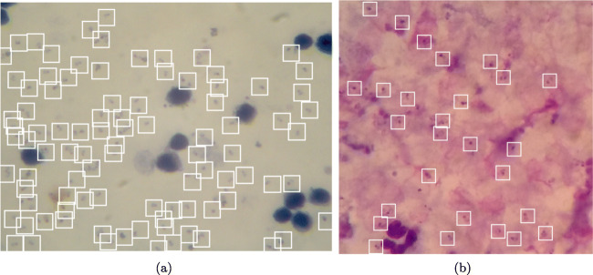
We train and evaluate our system using two datasets collected using low-cost devices; Dataset A¹ [12] contains images captured using a digital microscope camera mounted on a conventional light microscope, and Dataset B² [13] contains images captured using a mobile phone mounted on a conventional light microscope. Both datasets were annotated by experts using bounding boxes(coordinates on an image) each centered around a parasite as shown in Fig. 2. The coordinates of 49,900 Plasmodium falciparum parasites were recorded in 2703 images (1024 × 768 pixels) from 133 individuals in dataset A. The set of images in dataset A were taken from thick blood smears stained using Field stain at ×1000 magnification. The coordinates of 7628 Plasmodium falciparum parasites were recorded in 1182 images (750 × 750 pixels) in dataset B. The set of images in dataset B were also taken from thick blood smears stained using Giemsa stain at ×1000 magnification. The parasite of interest in both datasets is the Plasmodium falciparum. Each image in both datasets represents the maximum rectangular/square area of the microscopic field of view. It should be noted that the life state of the parasites in both datasets were not reported. Furthermore, the images are not labelled at patient level. Therefore, this study will not attempt to evaluate the performance at patient outcome level, instead the performance is evaluated at object level (i.e., number of parasites detected per image). We evaluate how well the model is able to detect all the parasites in each image in the test set.

Fig. 2.

Sample images annotated with bounding boxes. a Image sample from dataset A captured using a digital microscope camera. b Image sample from dataset B captured using a mobile phone

In both datasets, we randomly split images: 60% training, 20% validation, and 20% testing as illustrated in Table 2. The number of images that are negative (no parasites recorded) and positive (at least a parasite is recorded) from both datasets is not well balanced as shown in Table 2.

Table 2.

Datasets: Number of images (positive and negative) and parasite

	Dataset A			Dataset B
	+ images	– images	Parasites	+ images	– images	Parasites
Training	1458	164	30107	577	132	4728
Validation	481	59	10302	198	38	1510
Testing	479	62	9491	173	64	1390
Total	2418	285	49900	948	234	7628

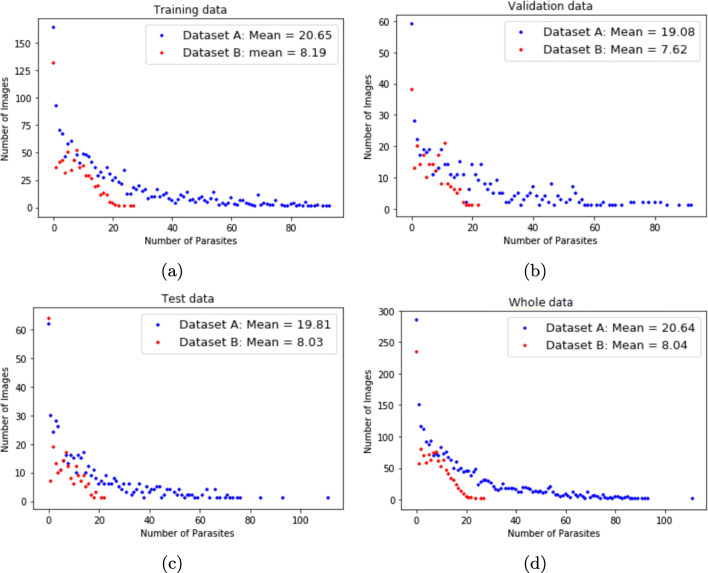
We show the parasite distribution in each image for both datasets in Fig. 3. Figure 3 a shows the parasite distribution in the training data with a mean number of parasite per image equal to 20.65 for dataset A and 8.19 for dataset B. Figure 3 b shows the parasite distribution in the validation data with a mean number of parasite per image equal to 19.08 for dataset A and 7.62 for dataset B. Figure 3 c shows the parasite distribution in the test data with a mean number of parasite per image equal to 19.81 for dataset A and 8.03 for dataset B. Figure 3 a shows the parasite distribution for the whole dataset with a mean number of parasite per image equal to 20.64 for dataset A and 8.04 for dataset B.

Fig. 3.

Parasite distribution per image. a Training data. b Validation data. c Test data. d Whole data

Training

As a result of the changes we have made to the architecture, we train our network from zero. The feature extraction network in YOLOv3 is trained separately on Imagenet [26] dataset before further training the full model for object detection. In our model, we train the feature extraction network and detection network from zero together at once. The images in the two datasets described in “Data” have different sizes. Therefore, instead of having a constant input image size, we change the network input size after every 10 training batches. All the input images are resized to dimensions which must be a multiple of 32 as we downsample an input image at 5 convolution operations using a stride of 2 during our feature extraction process. We randomly pick the input image size in range between 224 × 224 to 800 × 800 during training after every 10 batches. The input dimension must have equal height and width. The network input image size is changed on the fly during training without affecting the number of parameters in the model. This enables the network to learn to predict across different image resolutions. Therefore, our model enables us to make a trade off at test time between accuracy and computation cost/speed. The training data is heavily augmented due to imbalanced datasets and limited number of samples to avoid over fitting. We use the heavy augmentation option from the imgaug³ pipeline, and all the image augmentation is done randomly at runtime during training. We train the networks independently for each dataset to ensure that our model can learn from the images with high object-density as well as images with low object-density, as the two datasets have different distribution of parasites. In addition to parasite distribution, the two datasets were generated using different devices, and different stains were used. We do not perform image preprocessing at test apart from resizing the input image to a size W × H where W = H and multiple of 32.

We train our model using Tensorflow [27] and Keras [28] libraries. We use the standard RMSProp [29] optimizer with decay and momentum both set to 0.9. Every layer consists of a standard weight decay set to 4e − 1 as well as batch normalization. We set the initial learning rate at 0.0045 chosen after multiple experiments, and reduce the learning rate when it plateaus by factor 0.1. To speed up the training process, we use the NVIDIA GeForce GTX 1080 Ti GPU, as training a deep learning model is computationally expensive. Training the model has to be done only once, and retraining only periodically depending on the model performance in the real world environment. This trained model can be used on multiple low-resource client devices (cellphones, low-powered PCs) in the field without problems, since parasite detection and counting in novel images using an already trained model is much faster (several orders of magnitude cheaper, computationally not requiring GPUs) than retraining the model in the first place.

Evaluation

Evaluating object detection is non trivial, as there are two distinct tasks to measure: classification, which determines whether an object exists in the image, and localization which determines the location of the object (a regression task). In this study we use the average precision (AP) evaluation metric used in the Pascal visual object detection class (VOC) challenge [21] which is one of the most popular datasets for object detection. Currently, there are no standard object detection evaluation metrics tailored for microscopic objects; hence, we use the popular Pascal VOC AP. The AP used in the Pascal VOC challenge is an interpolated AP from [30] used for evaluating classification and detection. To calculate the AP, the precision-recall curve is computed from the model’s detection output by using the bounding box confidence score. Each predicted bounding box in an image/video has a confidence score. A detection is considered positive if the bounding box confidence score is above the certain score threshold. In this study, we maintain the Pascal VOC confidence score of more than 50%. The 50% confidence score threshold in this study gives us the optimal F1 score. Precision and recall are computed as shown in Eqs. 2 and 3 respectively.

$$Precision=\frac{TP}{TP+FP}$$ 2

$$Recall=\frac{TP}{TP+FN}$$ 3

where TP is true positive, FP is false positive, and FN is false negative. The TP, FP, and FN are determined as shown in Fig. 4. The final step in calculating the AP score is to compute the precision over all recall values. Therefore, AP summarizes the shape of the precision-recall curve and is determined as the mean precision at a set of eleven equally spaced recall levels [0.0,0.1,...,1.0]. The AP is then computed as shown in Eq. 4:

$$\begin{array}{rcl}AP=\frac{1}{11}\sum _{r\in R}Precision\left(Recal{l}_r\right);R=0.0,0.1,\mathrm{...},1.0& & \\ & & \end{array}$$ 4

Fig. 4.

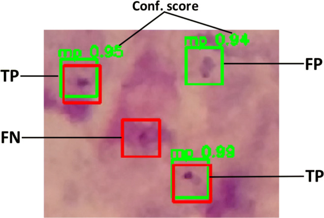
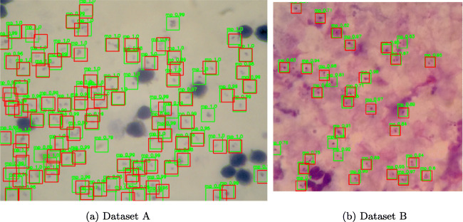
Prediction example. RED: true box annotated by experts. GREEN: predicted box by our model. The confidence score is the probability that our model assign to the predicted box that it contains a parasite

The precision at each recall level r is interpolated by getting the maximum precision recorded at recall that exceeds Recall_r:

$$Precision\left(Recal{l}_r\right)=\underset{\tilde{r}:\tilde{r}\ge r}{\max }Precision\left(Recal{l}_{\tilde{r}}\right)$$ 5

The precision-recall curve is interpolated to reduce the impact of jitter in the precision-recall curve that are caused due to small changes in the ranking of examples. This implies that to get higher AP score, the model must have precision at all levels of the recall. The model gets penalized if it only retrieves a subset of cases with high precision.

In order to evaluate the model on parasite localization in images or videos, there is a need to determine how well our model predicts the location of all the parasites. We archive this by drawing a bounding box around the parasite. Localization is evaluated by measuring the overlap ratio between the predicted bounding box and the ground truth bounding box. The overlap ratio is also known as Intersection over Union (IoU) computed as illustrated in Fig. 5a. We show different IoUs thresholds in Fig. 5. In this study, we set IoU threshold to 0.3. This means that if the overlap ratio between predicted box and true box is 0.3, we consider that detection as a TP. The threshold of 0.3 was set deliberately low to account for inconsistencies in bounding boxes in the ground truth data with regards to placing the parasite in the center of the box. We are confident that a threshold of 0.3 is sufficient to consider a positive detection as shown from the visual representation in Fig. 5b. The bounding boxes in dataset A are 50 × 50 pixels while in dataset B are 40 × 40 pixels.

Fig. 5.

Intersection over Unions (IoU) values. Red: True box annotated by experts. Green: predicted box

Results and Discussion

We compare the performance of our model against human experts and the baseline. We consider the sliding window plus convolutional neural network (SW + CNN) approach used in [13] as the baseline. We optimized our model in the best way possible for simplicity and detection speed. Earlier during model training, we manually examined random images to inspect the consistency in the annotation of images. This gave us an idea of what to expect when we test our model’s performance. We discovered some annotation errors in the few random sampled images. Therefore, in order to provide a fair and realistic model evaluation, we gave the test set images to two independent experts from different labs to annotate, and we evaluated the annotations. In the baseline model, parasite detection was not evaluated therefore we reimplemented the baseline model using the same libraries as our model for a fair performance comparison. The results are shown in Table 3.

Table 3.

Performance comparison at parasite level

Network	Input size	mAP: dataset A	mAP: dataset B	No. of parameters	CPU time/image
Modified YOLO	224 × 224	0.762	0.814	205,934	0.07 s
Modified YOLO	544 × 544	0.871	0.880	205, 934	0.20 s
Modified YOLO	800 × 800	0.887	0.902	205, 934	0.42 s
SW + CNN [13]	50 × 50 patch size	0.515	0.685	602,046	2.20 s
Human expert I	Original size	0.896	0.923	−	−
Human expert II	Original size	0.904	0.912	−	−

Our model outperforms the baseline on both datasets in every category. Our model performance on the two datasets is almost at par with human experts in terms of mean average precision (mAP) but our model is several orders of magnitude faster at detection. For the results in Table 3, the IoU threshold for our modified YOLO and human experts is set to 0.3 and the confidence score threshold is 0.5 while for the SW + CNN model, the IoU threshold is set to 0.15 and the detection probability threshold is 0.9 based on their implementation. The number of parameters in this case represents the total number of parameters in the feature extraction network and the detection network. The detection time represents the average amount of time our models takes to detect parasites in an image by predicting bounding boxes. The detection time is measured on a CPU.

To show the robustness of our model, we evaluate our model by interchanging the test dataset, a network trained on the training set A is evaluated on test set B and vice-versa without retraining the two networks. We show the results in Table 4. The results in Table 4 shows that our model is not significantly affected by the variability in the dataset such as change of camera and staining.

Table 4.

Model performance on swapped test sets

Network	Input size	mAP: train A - test B	mAP: train B - test A
Modified YOLO	224 × 224	0.645	0.703
Modified YOLO	544 × 544	0.721	0.781
Modified YOLO	800 × 800	0.801	0.832

Our model uses fewer parameters compared to the baseline model which makes our model faster. The sliding window approach used in the baseline has a draw back in that the model only sees a small fraction of an image, thus discarding important background information. The YOLO algorithm addresses the background differentiation issue and scales much better to larger datasets than SW + CNN. We show in Fig. 6 how the model predicts parasites’ locations in images. The images in Fig. 6 represent some of the images with the most dense parasites from both datasets. The observed maximum annotated parasites count per image is 112 in dataset A and 27 in dataset B.

Fig. 6.

Sample prediction by our model: Red boxes represents the true parasites, green boxes represent our model prediction with the confidence score. The input image is 544 × 544 and IoU = 0.3. No preprocessing is done at test time apart from resizing the images to a user desired input image size

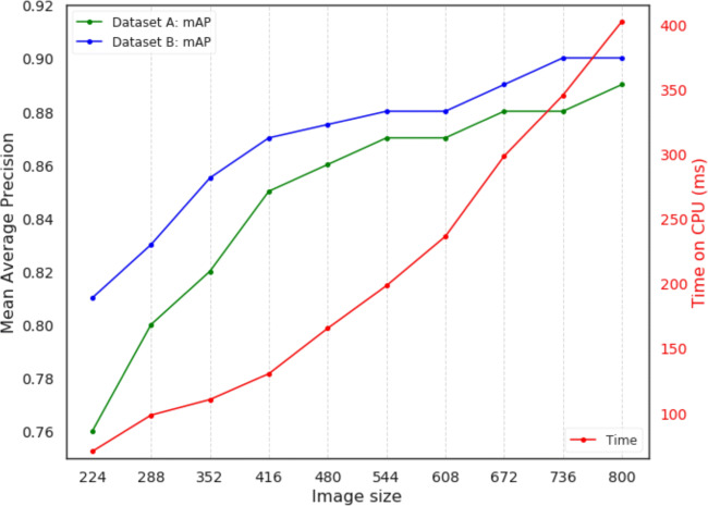
Our model is trained using different image input sizes from 224 × 224 pixels to 800 × 800 pixels. Therefore, at test time we make a trade off between accuracy and computational cost. Lowering the input size at test time affects the accuracy while increasing the input size increases the computational cost. We show this trade off in Fig. 7. The mean average precision increases with an increase in image size as shown in Fig. 7. However, increasing the input image size beyond 800 × 800 does not significantly improve the mAP. This can be attributed to parasite density in images and partially on model capacity. The denser the parasites are in images, the more the annotated bounding boxes overlap. Our model in some cases predict a single bounding box for parasites that are very close to each other. This has an effect on the way we evaluate the precision as two annotated parasites with more that 40% overlap between them are counted as a single parasite in our model. This problem can be resolved by reducing the size of the bounding box annotations, as we noticed that the parasites occupied less 50% area of annotated bounding box. An alternative approach would be to move beyond bounding box annotations to pixel segmentation which looks at the actual boundaries of the object of interest in an image.

Fig. 7.

Image input size versus Mean Average Precision versus versus time on a CPU in milliseconds; IoU = 0.3. The image size equal to width equal to height

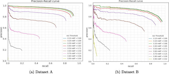
The mean average precision is affected by the overlap threshold set during detection. In Fig. 8, we show the precision-recall curves for both datasets to illustrate how the mean average precision is affected by different overlap thresholds. We start with the lowest overlap threshold, i.e., 0.1. For an IoU of 0.1, if the true box and predicted box are the same size, it means the overlap covers 17.5% of the true box which is large enough to consider a detection positive. During training, we consider a positive detection if the overlap (IoU) is more 0.3, which means that predicted box overlaps the true box by 52.5%.

Fig. 8.

Precision-recall curves for both dataset produced at different IoU thresholds. The image input size is 544 × 544, confidence score threshold is 0.5

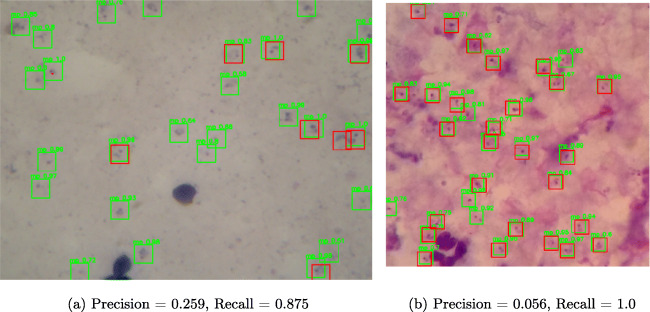
To better understand the worst case predictions by our model, we look at images with lowest precision from both datasets as shown in Fig. 9. In both cases, the model is very confident that these are parasites as can be seen from the confidence scores on the bounding boxes. In most cases, this can be attributed to missed labelling by the annotators as is the case in most supervised learning problems. We found that in most cases a few parasites were not annotated. Minor errors in bounding box annotations can significantly affect the performance of the model on the test set. This explains why the average precision for human experts is around 0.9 and also highlights the subjectivity of parasite quantification in blood smears.

Fig. 9.

Sample images from test set with lowest precision. a Image from dataset A. b Image from dataset B. Red boxes represents the true parasites, and green boxes represent our model prediction

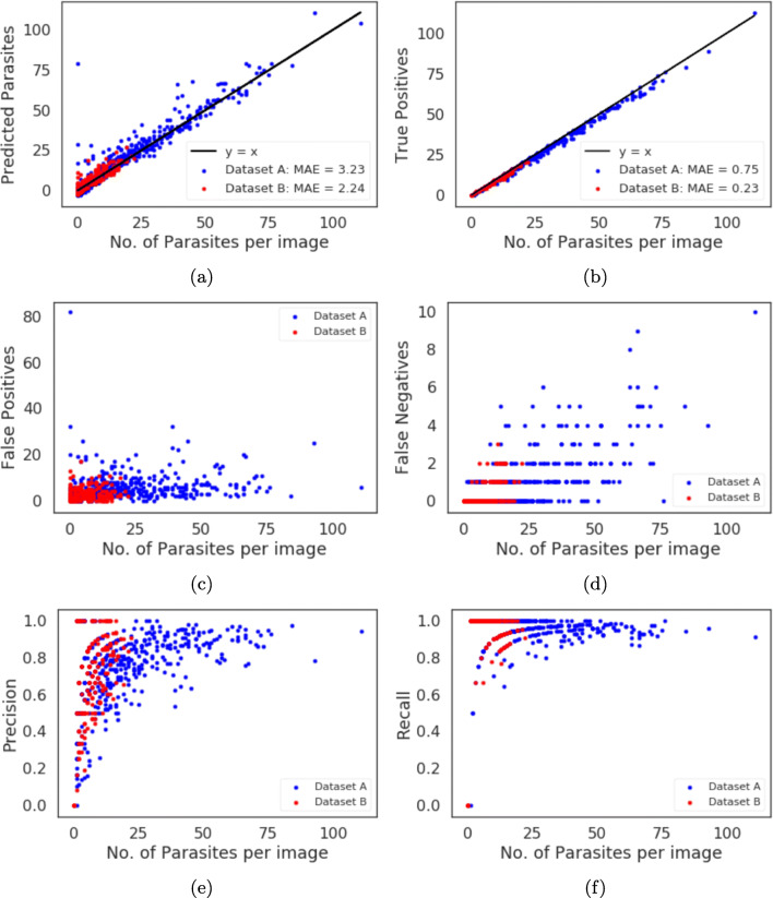
We further give an insight into our model prediction performance by looking at the number of parasites detected in each image. We show these results in Fig. 10. Figure 10 a shows true number of parasites in each image versus the number of parasites per image detected by our model. We fit a y = x line over the points in Fig. 10a for both datasets where x is the true number of parasites per image. We use mean absolute error (MAE) to assess our model prediction error. The MAE is 3.23 for dataset A and 2.24 for dataset B. We do the same for the total number of parasites per image versus the true positives per image in Fig. 10b. We fit a y = x line over the points for each dataset, the MAE is is 0.75 for dataset A and 0.23 for dataset B. Figure 10 c shows the total number of parasites per image versus the false positives per image and we can see that the false positives count decreases as the number of parasites in an image increases. For images with the low parasite count, the false positives’ ratio to total number of parasites is higher than images with high parasite count. This can be partially attributed to annotation errors as shown in the images with lowest precision in Fig. 9. Increasing the detection threshold could reduce the false positives but this will affect the sensitivity of the model. Figure 10 d shows the total number of parasites per image versus false negative per image and the results shows that as the images gets denser with parasites, the more chances some parasites will be missed by our model. Figures 10 e and f show the total number of parasites per image versus the precision per image and the recall per image respectively. At test time, the model allows for this flexibility where one can choose which metrics to maximize to get the best result for each particular case.

Fig. 10.

Different metrics in terms of number of parasites per image in the test set. The image input size is 544 × 544, confidence score threshold is 0.5. a True number of parasites per image vs number of predicted parasite by model per image. b True number of parasites per image vs model’s true positives per image. c True number of parasites per image vs model’s false positives per image. d True number of parasites per image vs model’s true negatives per image. e True number of parasites per image vs model’s precision per image. f True number of parasites per image vs model’s recall per image

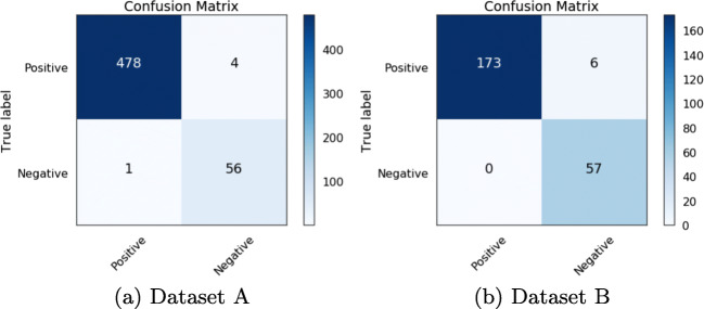
For overall image classification, we use the object detection results of each image. An image can be classified positive or negative by considering the precision, recall and accuracy from the parasite prediction count. The precision, recall, and accuracy can be affected by a number of factors such as the intersection over union, confidence score threshold, etc. We consider an image positive if the precision at object level is greater than zero. This means that at least a parasite is detected in an image. However, this may not give a true picture if we do not consider recall and accuracy as illustrated in the worst case result in Fig. 9b where the precision is 0.056 and the accuracy is 0.055. Such a result may not give a true diagnostic at patient level unless we consider multiple images which represents microscopic fields of view as recommended by the World Health Organization (WHO). Therefore, to perform classification at patient level, we need to analyze multiple images. The WHO recommends at least 100 fields of view (images) to consider a patient negative. Neither dataset has patient-level information for us to be able to apply patient-level evaluation metrics. We report the image level classification results using the confusion matrix in Fig. 11 and other classification metrics in Table 5. Our model achieved 99.07% and 97.46% accuracy on dataset A and dataset B respectively. By extrapolating these results to patient-level classification, if we apply our model to 100 images from a patient sample, the model should thus be able to classify with confidence as to whether a patient has malaria or not.

Fig. 11.

Classification results at image level in test datasets. The image input size is 544 × 544, confidence score threshold is 0.5

Table 5.

Model classification performance at image level

	Sensitivity	Specificity	Precision	F-score	Accuracy
Dataset A	0.9979	0.9333	0.9917	0.9948	0.9907
Dataset B	1.0000	0.9048	0.9665	0.9830	0.9746

Conclusion

This research provides a prototype for an inexpensive alternative to, and a complementary solution for, rapid malaria screening and can help to provide access to quality malaria diagnosis that is currently routinely unavailable in low-resource settings. Our solution can potentially be used as decision support tool for diagnostic consistency, help reduce the dependence on manual microscopic examination, relieve operator fatigue, and improve throughput rates. We evaluate the performance of our system on images that were generated using low-cost devices which include a mobile phone or digital microscope camera mounted on light microscope. The mean average precision on two test datasets is on par with human experts, but several orders of magnitude faster as we can process a single image in milliseconds using a simple mobile device. We demonstrate how a generic object detection algorithm can be repurposed for detecting very small objects which require skilled experts to accurately identify. Our system is able to detect and localize malaria parasites in thick blood smears with high precision and sensitivity.

Compliance with Ethical Standards

Conflict of Interests

The authors declare that they have no conflict of interest.

References

- 1.WHO (2018) World malaria report 2018, https://www.who.int/malaria/media/world-malaria-report-2018/en/
- 2.White NJ, Ho M: The pathophysiology of malaria. In: Advances in Parasitology, vol 31. Elsevier, 1992, pp 83–173 [DOI] [PubMed]
- 3.Kwiatkowski D, Sambou I, Twumasi P, Greenwood B, Hill A, Manogue K, Cerami A, Castracane J, Brewster D. Tnf concentration in fatal cerebral, non-fatal cerebral, and uncomplicated plasmodium falciparum malaria. The Lancet. 1990;336(8725):1201–1204. doi: 10.1016/0140-6736(90)92827-5. [DOI] [PubMed] [Google Scholar]
- 4.Organization W.H. (2016) Malaria microscopy quality assurance manual-version 2. World Health Organization
- 5.Petti CA, Polage CR, Quinn TC, Ronald AR, Sande MA. Laboratory medicine in africa: a barrier to effective health care. Clin Infect Dis. 2006;42(3):377–382. doi: 10.1086/499363. [DOI] [PubMed] [Google Scholar]
- 6.Moody A. Rapid diagnostic tests for malaria parasites. Clin Microbiol Rev. 2002;15(1):66–78. doi: 10.1128/CMR.15.1.66-78.2002. [DOI] [PMC free article] [PubMed] [Google Scholar]
- 7.Kim S, Nhem S, Dourng D, Ménard D. Malaria rapid diagnostic test as point-of-care test: study protocol for evaluating the vikia® malaria ag pf/pan. Malar J. 2015;14(1):114. doi: 10.1186/s12936-015-0633-3. [DOI] [PMC free article] [PubMed] [Google Scholar]
- 8.Hung J, Carpenter A: Applying faster r-cnn for object detection on malaria images. In: 2017 IEEE Conference on Computer Vision and Pattern Recognition Workshops (CVPRW). IEEE, 2017, pp 808–813 [DOI] [PMC free article] [PubMed]
- 9.Yang D, Subramanian G, Duan J, Gao S, Bai L, Chandramohanadas R, Ai Y. A portable image-based cytometer for rapid malaria detection and quantification. PloS one. 2017;12(6):e0179161. doi: 10.1371/journal.pone.0179161. [DOI] [PMC free article] [PubMed] [Google Scholar]
- 10.Pattanaik P, Swarnkar T, Sheet D: Object detection technique for malaria parasite in thin blood smear images. In: 2017 IEEE International Conference on Bioinformatics and Biomedicine (BIBM). IEEE, 2017, pp 2120–2123
- 11.Mehanian C, Jaiswal M, Delahunt C, Thompson C, Horning M, Hu L, McGuire S, Ostbye T, Mehanian M, Wilson B, et al: Computer-automated malaria diagnosis and quantitation using convolutional neural networks. In: Proceedings of the IEEE Conference on Computer Vision and Pattern Recognition, 2017, pp 116–125
- 12.Quinn JA, Andama A, Munabi I, Kiwanuka FN. Automated blood smear analysis for mobile malaria diagnosis. Mobile Point-of-Care Monitors and Diagnostic Device Design. 2014;31:115. [Google Scholar]
- 13.Quinn JA, Nakasi R, Mugagga PK, Byanyima P, Lubega W, Andama A: Deep convolutional neural networks for microscopy-based point of care diagnostics. In: Machine Learning for Healthcare Conference, 2016, pp 271–281
- 14.Neubeck A, Van Gool L: Efficient non-maximum suppression. In: ICPR 2006. 18th International Conference on Pattern Recognition, 2006, vol 3. IEEE, 2006, pp 850–855
- 15.Redmon J, Divvala S, Girshick R, Farhadi A: You only look once: unified real-time object detection. In: Proceedings of the IEEE Conference on Computer Vision and Pattern Recognition, 2016, pp 779–788
- 16.Liu W, Anguelov D, Erhan D, Szegedy C, Reed S, Fu C-Y, Berg AC: Ssd: single shot multibox detector. In: European Conference on Computer Vision. Springer, 2016, pp 21–37
- 17.Girshick R (2015) Fast r-cnn, arXiv preprint arXiv:1504.08083
- 18.Lin T-Y, Goyal P, Girshick R, He K, Dollár P (2017) Focal loss for dense object detection, arXiv preprint arXiv:1708.02002 [DOI] [PubMed]
- 19.Zhang S, Wen L, Bian X, Lei Z, Li SZ: Single-shot refinement neural network for object detection. In: Proceedings of the IEEE Conference on Computer Vision and Pattern Recognition, 2018, pp 4203–4212
- 20.Redmon J, Farhadi A (2018) Yolov3: an incremental improvement, arXiv preprint arXiv:1804.02767
- 21.Everingham M, Van Gool L, Williams CK, Winn J, Zisserman A. The pascal visual object classes (voc) challenge. Int J Comput Vis. 2010;88(2):303–338. doi: 10.1007/s11263-009-0275-4. [DOI] [Google Scholar]
- 22.Lin T-Y, Maire M, Belongie S, Hays J, Perona P, Ramanan D, Dollár P, Zitnick CL: Microsoft coco: common objects in context. In: European Conference on Computer Vision. Springer, 2014, pp 740–755
- 23.Chollet F (2016) Xception: deep learning with depthwise separable convolutions
- 24.Sandler M, Howard A, Zhu M, Zhmoginov A, Chen L-C (2018) Inverted residuals and linear bottlenecks: mobile networks for classification, detection and segmentation, arXiv preprint arXiv:1801.04381
- 25.Hartigan JA, Wong MA. Algorithm as 136: a k-means clustering algorithm. J R Stat Soc: Ser C: Appl Stat. 1979;28(1):100–108. [Google Scholar]
- 26.Deng J, Dong W, Socher R, Li L-J, Li K, Fei-Fei L: Imagenet: a large-scale hierarchical image database. In: CVPR 2009. IEEE Conference on Computer Vision and Pattern Recognition, 2009. IEEE, 2009, pp 248–255
- 27.Abadi M, et al.: Tensorflow: a system for large-scale machine learning. In: 12th USENIX Symposium on Operating Systems Design and Implementation (OSDI 16), 2016, pp 265– 283
- 28.Chollet F, et al (2015) Keras. https://github.com/fchollet/keras
- 29.Tieleman T, Hinton G. Lecture 6.5-rmsprop: divide the gradient by a running average of its recent magnitude. COURSERA: Neural Networks for Machine Learning. 2012;4(2):26–31. [Google Scholar]
- 30.Salton G, McGill MJ. Introduction to modern information retrieval. New York: McGraw-Hill Inc.; 1986. [Google Scholar]