Highlights
-
•
Mathematical and computational models are used to predict cases of COVID-19 in Mexico.
-
•
The data is obtained through the Daily Technical Report issued by the Mexican Ministry of Health.
-
•
Gompertz, Logistic and Artificial Neural Network perform the modeling of the cases confirmed by COVID-19 with an R2>0.999.
-
•
Logistic, Gompertz and inverse Artificial Neural Network predicts the maximum number of new daily cases on May 8th, June 25th and May12th, 2020, respectively.
-
•
The Gompertz, Logistic and inverse Artificial Neural Network models predict different number of cases of COVID-19 at the end of the epidemic.
Keywords: Gompertz model, Logistic model, inverse Artificial Neural Network model, COVID-19 modelling, COVID-19 prediction
Abstract
This work presents the modeling and prediction of cases of COVID-19 infection in Mexico through mathematical and computational models using only the confirmed cases provided by the daily technical report COVID-19 MEXICO until May 8th. The mathematical models: Gompertz and Logistic, as well as the computational model: Artificial Neural Network were applied to carry out the modeling of the number of cases of COVID-19 infection from February 27th to May 8th. The results show a good fit between the observed data and those obtained by the Gompertz, Logistic and Artificial Neural Networks models with an R2 of 0.9998, 0.9996, 0.9999, respectively. The same mathematical models and inverse Artificial Neural Network were applied to predict the number of cases of COVID-19 infection from May 9th to 16th in order to analyze tendencies and extrapolate the projection until the end of the epidemic. The Gompertz model predicts a total of 47,576 cases, the Logistic model a total of 42,131 cases, and the inverse artificial neural network model a total of 44,245 as of May 16th. Finally, to predict the total number of COVID-19 infected until the end of the epidemic, the Gompertz, Logistic and inverse Artificial Neural Network model were used, predicting 469,917, 59,470 and 70,714 cases, respectively.
1. Introduction
In December 2019, a new coronavirus disease emerged characterized as a viral infection with a high level of transmission in Wuhan, China. Coronavirus 19 (COVID-19) is caused by the virus known as Severe Acute Respiratory Syndrome coronavirus 2 (SARS-CoV-2) established by the Coronaviridae Study Group of the International Committee on Taxonomy of Viruses (ICTV) [1]. The origin of this virus is not yet confirmed, but a sequence-based analysis suggests bats as a possible key reservoir [2,3].
Furthermore the notorious effects that the virus has on people's health, there are other effects that are triggered as an indirect effects of the virus, some of these are the following: psychological distress, economic losses and negative impacts on daily activities [4]. Due to these effects, and in order to counteract them, the governments of different countries have made public policy decisions in both the health and economic aspects.
At the same time in the academic field, several research papers have been published focused on modeling and estimating the possible number of people infected with COVID-19 in a specific period. Ivanov [5] presented a robust simulation on the impact of COVID-19 on global supply chains, the results conclude in taking care of the closing and opening of the facilities at different levels could become an important factor that determines the impact of the epidemic outbreak. Li et al. [6] applied a Gaussian distribution to analyze COVID-19 transmission in Hubei Province of China and developed predictions on the epidemic trends in South Korea, Italy, and Iran, the results show the evolution of the epidemic, discovering that imposing controls would have a significant impact. Duccio Fanelli and Francesco Piazza [7] developed a mathematical model consisting of susceptible-infected-recovered-deaths (SIRDs) to analyze the outbreak of the coronavirus disease in China, Italy and France, the results describe that the recovery rate in the countries is the same, while the infection and mortality rates seem to be different. Petropoulos and Makridakis [8] presented an objective approach to predict the continuation of global COVID-19 using models from the exponential smoothing family, the results provide a forecast timeline for proper planning and decision making.
Applied mathematical models, such as Gompertz and Logistic, have been used successfully to predict the number of infected with COVID-19 in China, as demonstrated by: Jia et al [9] where three mathematical models were applied, including the Gompertz model and logistic model, to estimate the progress of COVID-19 in Wuhan, China, the results of the mathematical models predict that the COVID-19 will be over probably in late-April, 2020 in Wuhan. Castorina et al. [10] developed the mathematical Gompertz and Logistic models to evaluate the effectiveness of containment in the epidemic spread of COVID-19 in China, South Korea, Italy, and Singapore, the results of the models predict the maximum number of infected individuals for each country studied, in order to maintain a strong containment policy. Ahmadi et al. [11] analyzed the prediction of definitive cases of COVID-19 in Iran through mathematical models, the results show that, by carrying out compliance and public behavior interventions, it is possible to control and reduce the COVID-19 epidemic from April 28th to July 2020 in Iran through the Gompertz model. On the other hand, among computational models to simulate and predict non-linear behaviors, the inverse Artificial Neural Network (ANNi) has recently excelled. In the literature, the ANNi computational model has simulated and predicted values of interest in engineering fields, as reported by: Márquez-Nolasco et al. [12] developed two inverse artificial neural network models to simulate and estimate the internal heat and outlet temperature of a thermal absorber. The results show a good simulation of the process (R2 >0.99) and through the estimation it was possible to obtain higher values both in the internal heat and in the outlet temperature with respect to those obtained experimentally. Abdallah el hadj [13] used the inverse artificial neural network to estimate the equilibrium temperature, equilibrium pressure and critical temperature in the solubility of solid drugs in carbon dioxide in critical properties. The results show that the estimate obtained an average relative deviation of 1.1% when compared with properties reported in the literature.
Mexico has not escaped from the global pandemic, on February 27, 2020 the first patient with COVID-19 was reported in the country, meanwhile the day 22 of April the cases had already overcome the 10,000. Mexico is one of the country's most prone to the spread of the virus due to the number of patients who visit hospitals daily. For example, patients with chronic hemodialysis constitute a group at high risk of serious complications in case of presenting infections, due to their immunosuppressed state and the coexistence of significant comorbidities [14]. Likewise, other patients with various diseases are a potential spreading factor for COVID-19, basically to the fact that they regularly go to check-ups and wait in hospitals, exposing themselves to acquiring the infection.
Beside of the implementation of several public policies, the evolution of the epidemic in Mexico, has also motivated scientific research. In this regard, it is worth mentioning that research related to the estimation of the number of cases of COVID-19 becomes relevant due to the need to anticipate the sufficient infrastructure and specialized materials that are required to deal with treating the disease, such as: ventilation units, masks for the protection of health personnel, isolation rooms, among others.
An example of the academic research that was accomplished in Mexico is the one carried out by Cruz-Pacheco [15] where the arrival of the infectious outbreak in Mexico was estimated for a date between March 20 and 30, this estimate was made to strengthen the hospital infrastructure and the training of human resources in health. In addition, there are other studies about the evolution of the number of cases in Mexico, some of them were presented at the morning press conference of the Government of Mexico offered on April 16, 2020 [16], likewise, on April 13, 2020, researchers from the Autonomous Metropolitan University [17], offered an estimate of the maximum number of expected daily cases and total estimated cases at the end of the epidemic. However, as far as is known, there is no published article, that uses and contrasts "traditional" methods such as the Gompertz and Logistic models (using sigmoid functions), as well as modern methods such as direct and inverse Artificial Neural Network model, in the modelling and prediction of the number of confirmed cases of COVID-19 for México. Likewise, few studies analyze the inflexion point of the total cases curve, its growth rate and maximum level, which is why this article, when proposing alternative estimates, also tries to contribute to the robustness analysis of the existing estimations.
The predictions presented here are based on the data on the total number of cases confirmed by the Ministry of Health and come from the "Daily Technical Report" [18] issued by the Mexican Ministry of Health. In order, to modelling the actual tendency in the total number of confirmed cases, predict the number of total cases from May 9 to 16, and predict the total number of cases at the end of the epidemic, mathematical and computational models are proposed.
The rest of this article is organized as follows: in the section two, details about the sources and characteristics of the data are discussed. In section three, the mathematical and computational methodologies are specified, containing two subsections: the first dedicated to explain the specifications of mathematical models (Gompertz and Logistic), and the second, dedicated to explain the Computational Methodology, where the direct and inverse Artificial Neural Network model is presented. In section four the modeling analysis and prediction results are presented, this section is divided into two: one presenting the models and the prediction based on Gompertz and Logistic models, and the other is about the model and prediction based on inverse Artificial Neural Network. Finally, the last section presents the conclusions.
2. Data analysis
This section contains details of where the data was obtained as well as some specific characteristics related to them. The data used comes from the "Daily Technical Report" [18] issued by the Mexican Ministry of Health. Such report includes (among other data), figures on the number of total COVID-19 confirmed cases nationwide. The data presented in the report comes in turn from the information provided by the state health authorities. For each day, the figures correspond to those reported up to 1:00 p.m. It's very important to mention that the data on confirmed cases, only includes those cases that were successfully detected and reported, but the real total confirmed cases of COVID-19 are probably much higher (for example on the last April 8, 2020 the Ministry of Health declared that the total estimated confirmed cases could be around 8.3 times higher than the cases that were effectively registered [19]).
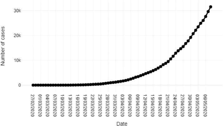
Fig. 1 shows the daily data on COVID-19 confirmed cases nationwide. This data includes 60 observations covering a period that goes from February 27, 2020 to May 8, 2020.
Fig. 1.
Confirmed Covid-19 Cases.
The figure shows values in a range that goes from 1 to 31,522 in a clear upward tendency. Considering the relative growth of cases an interesting fact is reveled: in the first 40 days the average growth rate on the number of cases is 25% per day, while in the last 20 days the average growth rate is just around 7% (maybe this could reflect at some extent the effects of containment policy carried out by the Ministry of Health).
The increasing levels of absolute growth suggest an exponential tendency with an average growth rate around 18% for the 72 observations, this confirms what is showed by the empirical evidence coming from several countries in earlier stages of the epidemic. However, it is important to mention that also the empirical evidence shows how in later stages of the epidemic, the growth rate on the total confirmed cases starts to slow down. These two patterns in the behavior, give as a result a kind of "Sigmoid" function in the shape of the complete tendency. So that´s why the Gompertz, Logistic an ANNi models are proposed to model and predict the confirmed cases.
3. Mathematical and computational methodology
In this section, the specifications of the mathematical and computational models to carry out the modeling and prediction of the cases of COVID-19 infection are described.
3.1. Mathematical methodology: Gompertz and Logistic models
3.1.1. Specification of the mathematical models
Mr. Gompertz [20] proposed in 1825 a model known as “Gompertz Theoretical law of mortality”. Since then, the Gompertz model has been used to describe growth in plants, animals, bacteria, and cancer cells.
Several re-parametrizations of this model have been made, one of them described in [21], that is very useful for analytic purposes, is the following:
| (1) |
On the other hand, the logistic growth model proposed by Verhulst in 1838 [22], can be expressed as a differential equation:
| (2) |
where:
Pg(t); Pl(t) are the dependents variables in the models (the population variable in both models)
cg; cl are the parameters for the growth rate in the models
kg; kl are the maximum values of each model attained as t goes to infinity
Eqs. (1) and (2) are differential equations, that can be solved to obtain:
| (3) |
| (4) |
where:
Tg; Tl are the t values that correspond to the inflexion point of the models (time at which the number of new confirmed cases per day begins to decrease)
3.1.2. Specification of the statistical models
From the deterministic relationships proposed by the mathematical models, the statistical relationships are formulated including a stochastic error term, this in order to be able to perform the empirical estimation of the model's parameters.
For Gompertz model
| (5) |
For Logistic model
| (6) |
where:
β g1; β l1 are the parameter estimates for kg and kl
β g2; β l2 are the parameter estimates for cg and cl
β g3; β l3 are the parameter estimates for Tg and Tj
and ɛgi; ɛli are the error terms for each model and represent the difference between the number of cases observed and the number of cases predicted by each model.
3.1.3. Non-linear least-squares method
From (5) and (6) equations, ɛgi and ɛli can be solved, to obtain:
For Gompertz model
| (7) |
For Logistic model
| (8) |
In order to find out the values that minimize the following sums of the m square errors, corresponding to the m observations, for each model: and
From an initial approximation and using the Gauss-Newton algorithm for the solution of non-linear least-squares problems, the values that minimize such sums can be found. All calculations were carried out with Stata.
3.2. Computational methodology: direct and inverse Artificial Neural Network
The direct and inverse Artificial Neural Network model is a set of coupled computational models that allow modeling and extrapolating values through a series of representative data. For the development of ANNi model, it is necessary to apply the coefficients obtained during the learning of an Artificial Neural Network (ANN) model in order to propose an objective function [23]. The steps to apply the computational methodology are the following:
3.2.1. Propose an ANN model
The ANN model is developed using a three-layer architecture. In the input layer, each input parameter (In) is assigned a weight factor (Wi) and the sum of these, a factor known as bia (b1) is added. In the hidden layer, a transfer function is applied to represent an internal output. In the output layer, the weighted sum of the signals provided by the hidden layer is calculated and output coefficients (Wo and b2) are added to generate a simulated value. The following Eq. (9) represents an ANN model using a tangential-sigmoidal function (TANSIG) on the hidden layer and a linear transfer function (PURELIN) the output layer:
| (9) |
Where: s is the neurons number in the hidden layer, k is the neurons number in the input layer and Out is the modeled value.
Generally, to carry out the learning a Levenberg-Marquardt algorithm is used due to its precision and speed when adjusting the coefficients to obtain the desired output [24]. All calculations were carried out with Matlab mathematical software with the ANN toolbox. The input data were divided into subsets of training, validation, and testing, where each contained 60%, 20%, and 20% of randomly selected samples, respectively. For training, the input and output variables were normalized. The output values were divided by 1000 and the input values were normalized in an interval of [0.1-0.9] applying the following Eq. (10):
| (10) |
3.2.2. Approach of the ANNi model
Once the ANN model has been developed, it is inverted to propose an objective function. This approach allows extrapolating input values (Inx) from a desired output (Out). The following Eq. (11) represents an objective function:
| (11) |
3.2.3. Resolution of the objective function
Once the ANNi model has been proposed, it is necessary to apply an optimization algorithm to find the values that solve the objective function in the shortest possible time. In this work, a genetic algorithm (GA) was coupled due to its search capacity and reasonable response time [25]. All calculations were carried out with Matlab mathematical software with the optimization toolbox.
3.3. Statistical criteria applied to the models
The Coefficient of Determination R2 is applied to specify the fit of the observed data and the modeled ones.
| (12) |
Where , is the average output value obtained by the model, and x out, obs is the observed output value.
4. Modeling analysis and prediction results
4.1. Modeling and prediction based on Gompertz and Logistic models
Eq. (13) shows the estimated Gompertz model
| (13) |
where:
is the number of total estimated COVID-19 cases for each day ti
469916.6 is the number of maximum estimated COVID-19 cases at the end of the epidemic
0.0208709 is the estimated growth rate of total COVID-19 cases
119.7037 is the time at which the maximum number of new daily cases is expected to occur
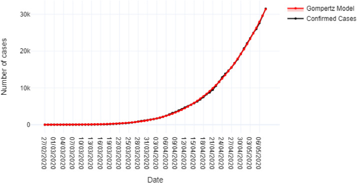
Fig. 2 shows the observed data on total COVID-19 cases, as well as the estimated data by Gompertz model from February 27th, to May 8th. The estimates of the model show a good fit as is indicated by an R2 coefficient of 0.9998.
Fig. 2.
Comparison between COVID-19 confirmed cases and those modeled by the Gompertz model.
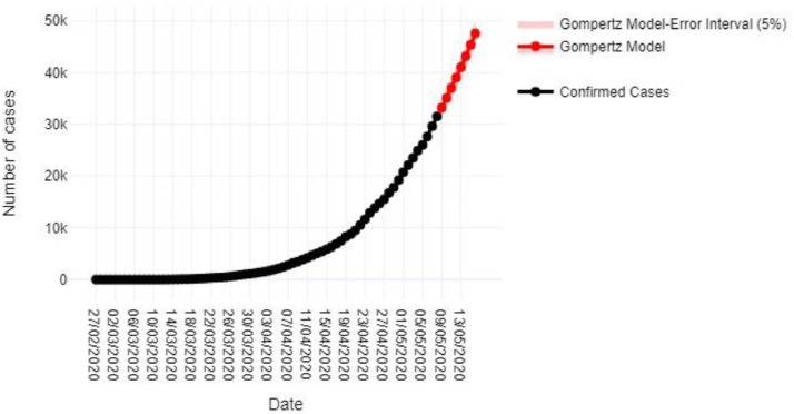
Regarding to the predicted values of the model for the period that goes from May 9th, to May 16th, Fig. 3 shows predicted value of 47,576 on May 16th.
Fig. 3.
Application of the Gompertz model to predict the number of COVID-19 cases from May 9th to 16th.
Also, this model predicts that the maximum number of total cases at the end of the epidemic (469,917) will be reached.
On the other hand, Eq. (14) shows the estimated Logistic model
| (14) |
where:
is the number of total estimated COVID-19 cases for each day ti
59, 470.15 is the number of maximum estimated COVID-19 cases at the end of the epidemic.
0.100822 is the estimated growth rate of total COVID-19 cases.
71.19428 is the time at which the maximum number of new daily cases is expected to occur.
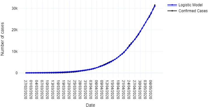
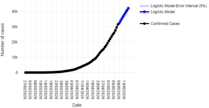
Fig. 4 shows the observed data on total COVID-19 cases, as well as the estimated data by Logistic model from February 27th, to May 8th. The estimates of the model show a good fit as is indicated by an R2 coefficient of 0.9996.
Fig. 4.
Comparison between COVID-19 confirmed cases and those modeled by the Logistic model.
Regarding to the predicted values of the model for the period that goes from May 9th, to May 16th, Fig. 5 shows a predicted value of 42,131 on May 16th
Fig. 5.
Application of the Logistic model to predict the number of COVID-19 cases from May 9th to 16th.
Also, this model predicts that the maximum number of total cases at the end of the epidemic (59,470) will be reached by the day 199, that is on September 12th.
Comparing Gompertz and Logistic models is very easy to note that the Logistic model results seems to be more plausible, considering the total number of cases at the end of the epidemic, also the inflexion point estimated by Logistic model (May 8t h) is according to that forecasted by the Ministry of health (May 8th), whereas according to the Gompertz Model, the inflexion point will be presented until June, 25th. So, Logistic model is the preferred over the Gompertz model.
4.2. Modeling and prediction based direct and inverse artificial neural network
An ANN model with seven neurons in the hidden layer and using a TANSIG function was able to model the number of COVID-19 infected registered until May 8th. Table 1 shows the coefficients of weights and bias obtained during training.
Table 1.
Obtained parameters of weights and biases for the ANN model.
| Number of neurons (s) | Weights |
Bias |
||
|---|---|---|---|---|
| Hidden layer (Wi) | Output layer (Wo) | b1 | b2 | |
| 1 | -17.2423 | 13.7590 | 30.3522 | 21.7621 |
| 2 | 4.2360 | 34.9032 | -3.9582 | |
| 3 | 130.9209 | 0.3591 | -94.4942 | |
| 4 | 25.3984 | 0.3621 | -14.0726 | |
| 5 | -53.5445 | -0.1005 | 22.9163 | |
| 6 | -32.9832 | -0.0522 | 11.2251 | |
| 7 | -6.2240 | 0.2387 | 1.8207 | |
s is the number of neurons in the hidden layer
The coefficients obtained are integrated into the following Eq. (15) to model the number of positive cases (N°) for COVID-19 infection:
| (15) |
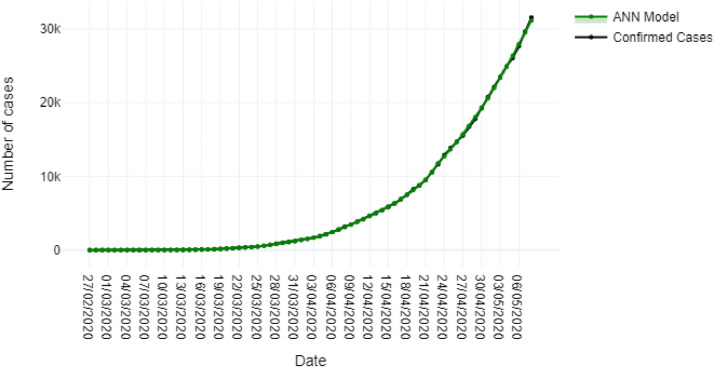
Fig. 6 shows the observed data on total COVID-19 cases, as well as the estimated data by ANN model from February 27th, to May 8th. The agreement between the confirmed and the modeled cases was satisfactory, obtaining a value of R2 = 0.9999.
Fig. 6.
Comparison between the COVID-19 confirmed cases and those modeled by the ANN model.
To carry out the prediction, an ANNi model was developed based on a similar procedure to that reported by Márquez et al. [12]. To predict the number of positive cases for the period that goes from May 9th to 16th, the following objective function was proposed using the coefficients presented in Table 1:
| (16) |
Where: Inx represents the number of days to extrapolate and N° represents the total number of positive cases of COVID-19.
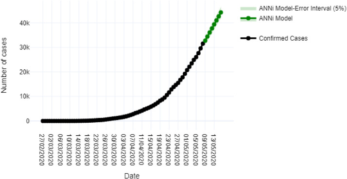
The genetic algorithm was applied to search the total number of positive cases for COVID-19 with respect to the number of extrapolated days. Fig. 7 shows the prediction of the number of cases by COVID-19 to be presented on May 16th obtained by ANNi.
Fig. 7.
Application of the ANNi model to predict the number of COVID-19 cases from May 9th to 16th.
Regarding to the predicted values of the model for the period that goes from May 9th, to May 16th, Fig. 7 shows a predicted value of 44,245 on May 16th. Comparing the computational model with the mathematical models, better modeling is denoted by the ANN model. Finally, this model predicts that the maximum number of total cases at the end of the epidemic (70,714) will be reached by the day 133, that is on July 8th. The inflexion point will be presented until May 12th.
5. Conclusions
In this paper are applied two mathematical models and a computational one, in order to estimate the COVID-19 cases. The results of the modelling show a good fit between the estimated and the observed data on total confirmed cases, given as a result an R2 of 0.9998, 0.9996 and 0.9999 for Gompertz, Logistic and Artificial Neural Networks models, respectively. Also, for May 16th a total of 47,576, 42,131 and 44,245 cases are predicted by each model. For the end of the epidemic a total of 469,917, 59,470 and 70,714 cases are predicted by each model. It´s important to mention that Logistic model, predicts a maximum of 1,498 new daily cases by May 8th (that is the inflexion point of the total cases curve),the Gompertz model, predicts a maximum of new daily cases of 3,607.90 by June 25th, the inverse Artificial Neural Network predicts a maximum of new daily cases of 1,665 by May 12th, whereas the Ministry of Health has estimated May 8th as the date for which the maximum of new daily cases will be attained.
The predicted results from the models could differ in a significant way from the observed ones, if there is a change in the coming days due to various testing strategies, social-distancing policies, reopening the community, or stay-home policy, the predicted death tolls will definitely change. Obviously, further analysis in broader validation of this conclusion is needed by updating the real current COVID-19 data into the model.
CRediT authorship contribution statement
O. Torrealba-Rodriguez: Conceptualization, Methodology, Data curation, Writing - review & editing, Project administration. R.A. Conde-Gutiérrez: Software, Validation, Investigation, Writing - original draft, Supervision. A.L. Hernández-Javier: Formal analysis, Resources, Visualization, Funding acquisition.
Declaration of Competing Interest
The authors declare that they have no known competing financial interests or personal relationships that could have appeared to influence the work reported in this paper.
Acknowledgements
The correspond author thanks at SNI CONACyT for the support provided.
References
- 1.Gorbalenya A.E., Baker S.C., Baric R.S. The species severe acute respiratory syndrome-related coronavirus: classifying 2019-nCoV and naming it SARS-CoV-2. Nat Microbiol. 2020;5:536–544. doi: 10.1038/s41564-020-0695-z. [DOI] [PMC free article] [PubMed] [Google Scholar]
- 2.Shereen M.A., Khan S., Kazmi A., Bashir N., Siddique R. COVID-19 infection: origin, transmission, and characteristics of human coronaviruses. J Adv Res. 2020;24:91–98. doi: 10.1016/j.jare.2020.03.005. [DOI] [PMC free article] [PubMed] [Google Scholar]
- 3.Cui J., Li F., Shi Z.L. Origin and evolution of pathogenic coronaviruses. Nat Rev Microbiol. 2019;17(3):181–192. doi: 10.1038/s41579-018-0118-9. [DOI] [PMC free article] [PubMed] [Google Scholar]
- 4.Zowalaty M.E.E., Jarhult J.D. From SARS to COVID-19: a previously unknown SARS-related coronavirus (SARS-CoV-2) of pandemic potential infecting humans–call for a one health approach. One Health. 2020;9 doi: 10.1016/j.onehlt.2020.100124. [DOI] [PMC free article] [PubMed] [Google Scholar]
- 5.Ivanov D. Predicting the impacts of epidemic outbreaks on global supply chains: a simulation-based analysis on the coronavirus outbreak (COVID-19/SARS-CoV-2) case. Transp Res E Logist Transp Rev. 2020;136 doi: 10.1016/j.tre.2020.101922. [DOI] [PMC free article] [PubMed] [Google Scholar]
- 6.Li L., Yang Z., Dang Z. Propagation analysis and prediction of the COVID-19. Infect Dis Model. 2020;5:282–292. doi: 10.1016/j.idm.2020.03.002. [DOI] [PMC free article] [PubMed] [Google Scholar]
- 7.Fanelli D., Piazza F. Analysis and forecast of COVID-19 spreading in China, Italy and France. Chaos, Solitons Fract. 2020;134 doi: 10.1016/j.chaos.2020.109761. [DOI] [PMC free article] [PubMed] [Google Scholar]
- 8.Petropoulos F., Makridakis S. Forecasting the novel coronavirus COVID-19. PLoS One. 2020;15(3) doi: 10.1371/journal.pone.0231236. [DOI] [PMC free article] [PubMed] [Google Scholar]
- 9.L. Jia, K. Li, Y. Jiang, X. Guo, T. ZhaoPrediction and analysis of coronavirus disease 2019. arXiv preprint arXiv:2003.05447. (2020)
- 10.P. Castorina, A. Iorio, D. Lanteri, Data analysis on coronavirus spreading by macroscopic growth laws. arXiv preprint arXiv:2003.00507 (2020).
- 11.Ahmadi A., Shirani M., Rahmani F. Modeling and forecasting trend of COVID-19 epidemic in Iran. medRxiv. 2020 doi: 10.34171/mjiri.34.27. [DOI] [PMC free article] [PubMed] [Google Scholar]
- 12.Márquez-Nolasco A., Conde-Gutiérrez R.A., Hernández J.A., Huicochea A., J.Siqueiros O.Rodriguez. Optimization and estimation of the thermal energy of an absorber with graphite disks by using direct and inverse neural network. J Energy Resour Technol. 2017;140(2):1–13. [Google Scholar]
- 13.Abdallah el hadj A., Laidi M., Si-Moussa C., Hanini S. Novel approach for estimating solubility of solid drugs in supercritical carbon dioxide and critical properties using direct and inverse artificial neural network (ANN) Neural Comput Appl. 2017;28(1):87–99. [Google Scholar]
- 14.Vega-Vega O., Arvizu-Hernández M., Domínguez-Cherit J., Sierra-Madero J., Correa-Rotter R. Salud Pública de México; 2020. Prevención y control de la infección por coronavirus SARS-CoV-2 (Covid-19) en unidades de hemodiálisis. [DOI] [PubMed] [Google Scholar]
- 15.Cruz-Pacheco G., Bustamante-Castaneda F.J., Caputo J.G., Jimenez-Corona M.E., Ponce-de-Leon S. Dispersion of a new coronavirus SARS-CoV-2 by airlines in 2020: Temporal estimates of the outbreak in Mexico. medRxiv. 2020 doi: 10.24875/RIC.20000113. [DOI] [PubMed] [Google Scholar]
- 16.Rivera C. Temas de la conferencia sobre el covid-19 en México del 16 de abril. Milenio. 2020, abril 16 https://www.milenio.com Recuperado de: [Google Scholar]
- 17.UAM. (2020, abril 13). Académicos de la uam proyectan la trayectoria del COVID-19. Recuperado 13 de abril de 2020, dehttp://www.comunicacionsocial.uam.mx/boletinesuam/227-20.html
- 18.Coronavirus (COVID-19)-Comunicado Técnico Diario. (2020, Abril 25). Recuperado el 26 de abril de 2020, desdehttps://www.gob.mx/salud/documentos/coronavirus-covid-19-comunicado-tecnico-diario-238449.
- 19.Monroy, M.V.y.J. (2020, April 9). Cifra real de infectados por Covid-19 en México sería de 26,519 personas, reconoce la Secretaría de Salud. Recuperado el 25 de abril de 2020, desde:https://www.eleconomista.com.mx/politica/Mexico-llega-al-Miercoles-Santo-con-3181-contagios-y-174-muertes-por-coronavirus-20200408-0113.html.
- 20.B. Gompertz, XXIV. On the nature of the function expressive of the law of human mortality, and on a new mode of determining the value of life contingencies. In a letter to Francis Baily, Esq. FRS &c. Philosophical transactions of the Royal Society of London, (115), 513-583. (1825) [DOI] [PMC free article] [PubMed]
- 21.Tjørve K., Tjørve E. The use of Gompertz models in growth analyses, and new Gompertz-model approach: an addition to the Unified-Richards family. PLoS One. 2017;12(6) doi: 10.1371/journal.pone.0178691. [DOI] [PMC free article] [PubMed] [Google Scholar]
- 22.Verhulst P.F. Notice sur la loi que la population poursuit dans son accroissement. Corresp, Math Phys. 1838;10:113–121. [Google Scholar]
- 23.Hernández J.A. Optimum operating conditions for heat and mass transfer in foodstuffs drying by means of neural network inverse. Food Control. 2009;20(4):435–438. [Google Scholar]
- 24.Mukherjee I., Routroy S. Comparing the performance of neural networks developed by using Levenberg–Marquardt and Quasi-Newton with the gradient descent algorithm for modelling a multiple response grinding process. Expert Syst Appl. 2012;39(3):2397–2407. [Google Scholar]
- 25.Hollande J.H. University of Michigan Press; 1975. Adaptation in natural and artificial systems; p. 183. [Google Scholar]


