Single-cell multiomic analysis identifies regulatory programs in mixed-phenotype acute leukemia

Abstract

Identifying the causes of human diseases requires deconvolution of abnormal molecular phenotypes spanning DNA accessibility, gene expression and protein abundance^1–3. We present a single-cell framework that integrates highly multiplexed protein quantification, transcriptome profiling and analysis of chromatin accessibility. Using this approach, we establish a normal epigenetic baseline for healthy blood development, which we then use to deconvolve aberrant molecular features within blood from patients with mixed-phenotype acute leukemia^4,5. Despite widespread epigenetic heterogeneity within the patient cohort, we observe common malignant signatures across patients as well as patient-specific regulatory features that are shared across phenotypic compartments of individual patients. Integrative analysis of transcriptomic and chromatin-accessibility maps identified 91,601 putative peak-to-gene linkages and transcription factors that regulate leukemia-specific genes, such as RUNX1-linked regulatory elements proximal to the marker gene CD69. These results demonstrate how integrative, multiomic analysis of single cells within the framework of normal development can reveal both distinct and shared molecular mechanisms of disease from patient samples.

To identify pathologic features within neoplastic cells, we first aimed to establish molecular features of normal development for comparison. As mixed-phenotype acute leukemias (MPALs) present with features of multiple hematopoietic lineages, we first constructed independent immunophenotypic, transcriptomic and epigenetic maps of normal blood development using droplet-based cellular indexing of transcriptomes and epitopes by sequencing (CITE-seq)⁶ (combined single-cell antibody-derived tag and RNA sequencing) and single-cell assay for transposase-accessible chromatin using sequencing (scATAC-seq; single-cell chromatin-accessibility profiling)⁷ on bone marrow and peripheral blood mononuclear cells (BMMCs and PBMCs, respectively; Fig. 1a). For CITE-seq analyses, we simultaneously generated 10x Genomics 3′ single-cell RNA sequencing⁸ (scRNA-seq) and antibody-derived tag sequencing⁶ (scADT-seq; Supplementary Table 3) libraries from 35,882 BMMCs (n = 12,602), CD34⁺-enriched BMMCs (n = 8,176) and PBMCs (n = 14,804). On average, 1,273 informative genes (2,370 unique transcript molecules) were detected per cell and replicates were highly correlated (Supplementary Fig. 1a–e). We then selected a feature set of transcripts to mitigate batch effects and linearly projected retained transcript counts into a lower-dimensional space using latent semantic indexing^9[,10 (LSI; Methods). Cells were clustered using Seurat’s shared nearest neighbor (SNN) approach¹¹, annotated using a manually curated maker gene list and visualized using uniform manifold approximation and projection (UMAP)¹² (Fig. 1b and Supplementary Fig. 1f).

Fig. 1 |. Multiomic epigenetic and phenotypic analysis of human hematopoiesis.

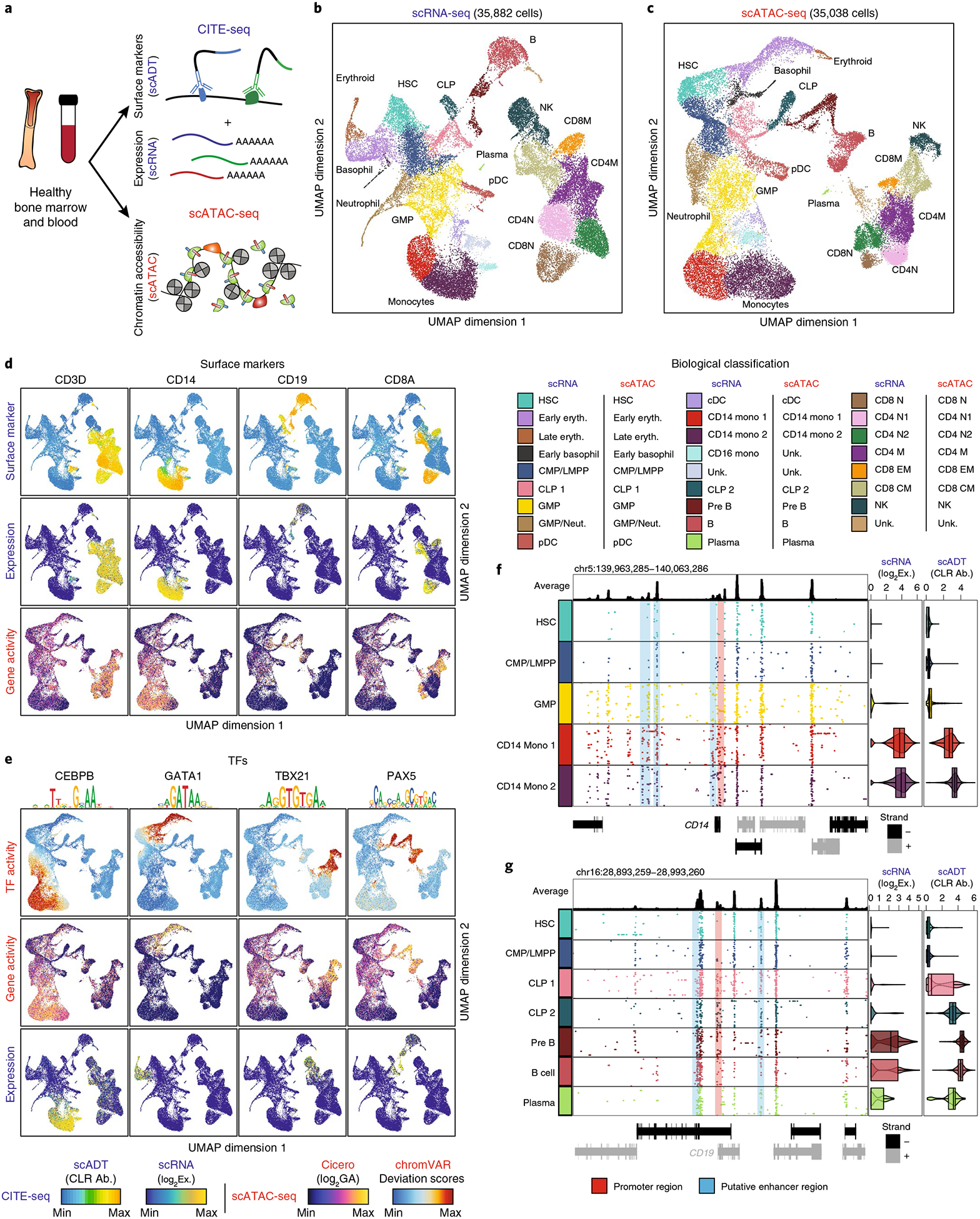
a, Schematic of multiomic profiling of chromatin accessibility, transcription and cell-surface antibody abundance on healthy bone marrow and PBMCs using CITE-seq (combined single-cell RNA and antibody-derived tag sequencing for each single cell, scRNA-seq and scADT-seq, respectively) and scATAC-seq. b, scRNA-seq LSI UMAP projection of 35,882 single cells across healthy hematopoiesis. Below are the biological classifications for the scRNA-seq clusters (see Supplementary Table 1). c, Top, scATAC-seq LSI UMAP projection of 35,038 single cells across healthy hematopoiesis. Bottom, the biological classifications for the scATAC-seq clusters (see Supplementary Table 1). d, Surface-marker overlay on single-cell RNA UMAP (as in b) of ADT antibody signal (top; center-log ratio (CLR) normalized), single-cell RNA (middle; log₂(gene expression) (Exp)) and single-cell ATAC log₂(gene-activity scores (GA)) for CD3D, CD14, CD19 and CD8A (bottom). e, TF overlay on single-cell ATAC UMAP (as in c) of TF chromVAR deviations (top), gene-activity scores (middle) and single-cell RNA for CEBPB, GATA1, TBX21 and PAX5 (bottom). f,g, Multiomic track of CD14 (specific in these clusters for monocytes) across monocyte development from HSC progenitor cells (f; n = 1,425–4,222) and multiomic track of CD19 (specific in these clusters for pre-B cells) across B cell development (g; n = 62–2,260). Multiomic tracks; average track of all clusters displayed (left top), binarized 100 random scATAC-seq tracks for each locus at a resolution of 100 bp (left bottom), scRNA-seq log₂ violin and box plots of normalized expression for each cluster and scADT-seq CLR violin and box plots of protein abundance for each cluster (right). Violin plots represent the smoothed density of the distribution of the data. In box plots, the lower whisker is the lowest value greater than the 25% quantile minus 1.5 times the interquartile range (IQR), the lower hinge is the 25% quantile, the middle is the median, the upper hinge is the 75% quantile and the upper whisker is the largest value less than the 75% quantile plus 1.5 times the IQR.

We next established an epigenetic map of normal hematopoiesis by measuring chromatin accessibility across 35,038 single BMMCs (n = 16,510), CD34⁺ BMMCs (n = 10,160) and PBMCs (n = 8,368) using droplet scATAC-seq (10x Genomics)⁷. These cells exhibited a canonical fragment-size distribution with clearly resolved sub-, mono- and multinucleosomal modes, a high signal-to-noise ratio at transcription start sites (TSSs), an average of 11,597 uniquely accessible fragments per cell on average, a majority (61%) of Tn5 insertions aligning within peaks and high reproducibility across replicates (Supplementary Fig. 2a–h). Using LSI, Seurat’s SNN clustering and UMAP, we generated a chromatin-accessibility map of hematopoiesis that complements the transcriptional map of hematopoiesis (Fig. 1c and Supplementary Fig. 2i).

To validate the proposed transcriptomic and epigenetic single-cell maps of hematopoiesis, we directly visualized lineage-restricted cell-surface marker and transcription-factor (TF) enrichment across each map. As anticipated, both scADT- and scRNA-seq measurements of surface makers demonstrate CD3D enrichment across bone marrow and peripheral T cells; CD14 enrichment within the monocytic lineage; broad up regulation of CD19 across the B cell lineage; and CD8A enrichment within cytotoxic T lymphocytes¹³ (Fig. 1d). Estimates of gene activity on the basis of correlated variation in promoter and distal-peak accessibility (Cicero¹⁴) broadly recapitulates this pattern, confirming that lineage specification is consistently reflected across the phenotypic, transcriptional and epigenetic maps of hematopoietic development (Fig. 1d). We then visualized our scADT-seq data of BMMCs and PBMCs using UMAP and found that we could broadly recapitulate our transcriptomic hematopoietic map (Supplementary Fig. 1g,h). To further support these cell-type identifications and developmental mappings, we show concordance between three separate single-cell measurements, including direct transcript measurements from the scRNA-seq dataset, inferred gene-activity scores from the scATAC-seq dataset and TF activity using chromVAR¹⁵, for key developmental TFs, including CEBPB in monocytic development, GATA1 within the erythroid lineage and TBX21 in NK and CD8⁺ T memory cells, as well as PAX5 in B cell and plasmacytoid dendritic cell development (Fig. 1e). High-resolution single-cell multiomic tracks for key marker genes in each of the identified lineages further support these identifications (Fig. 1f,g and Supplementary Fig. 3a–h). Collectively these results show that the proposed multiomic maps of healthy hematopoiesis are consistent and broadly capture essential phenotypic, transcriptomic and epigenetic features of blood development.

Recent work has shown that immunophenotypically distinct subpopulations of MPAL blasts have similar genomic lesions within a patient, and that cells from one lineage can reconstitute the alternate lineage in xenograft models¹⁶, suggesting that MPAL lineage plasticity may be epigenetically regulated. To explore the nature of this regulatory and phenotypic dysfunction, we assayed six MPAL samples including three T-myeloid MPALs (MPAL1-MPAL3), 1 B myeloid MPAL (MPAL4) and one T-myeloid MPAL sampled before CALGB chemotherapy (MPAL5) and after post-treatment relapse (MPAL5R) (Supplementary Table 1). Across these samples, we observed extensive immunophenotypic heterogeneity (via diagnostic flow cytometry analysis) including bilineal patterns (multiple blast populations expressing both lymphoid and myeloid lineage antigens), biphenotypic patterns (a dominant blast population that simultaneously expresses both lymphoid and myeloid antigens) and both patterns (Supplementary Fig. 4a–f). We then performed whole-exome sequencing (WES) and found mutational profiles similar to previous studies^16,17 (Supplementary Fig. 4g). To further profile our MPAL samples, we performed CITE-seq (18,056 cells) and scATAC-seq (35,423 cells) on either peripheral blood or bone marrow aspirates from these patients with MPAL, observing reasonable data quality per cell as compared to that obtained for healthy samples (Supplementary Fig. 5a–m).

Using our transcriptomic and chromatin landscapes of healthy hematopoiesis, we next sought to develop an analytical framework to identify the hematopoietic developmental signature at single-cell resolution. First, the chromatin and gene expression signatures of single cells are projected into the LSI subspace of our ATAC- and RNA-based healthy hematopoietic map, and the results are then visualized using UMAP (Fig. 2a and Supplementary Fig. 6a). Next, by determining the closest hematopoietic cells to the projected cells we can identify the hematopoietic developmental compartment. This method does not require defining discrete cell-type boundaries and uses a large feature set to robustly position cells within the continuous landscape of hematopoiesis. To validate this approach, we first projected downsampled published bulk RNA-seq and ATAC-seq data¹⁸ from subpopulations identified by fluorescence-activated cell sorting (FACS) into our chromatin and transcription hematopoietic maps and found high concordance with our healthy hematopoietic map and cluster definitions (Supplementary Fig. 6b). To further validate our approach, we projected published scRNA-seq¹⁹ and scATAC-seq^20–22 data from different platforms and different genomes on our chromatin and transcription hematopoietic maps and found striking agreement (Supplementary Fig. 6c). Lastly, we used our iterative LSI approach on 299,337 cells from the Human Cell Atlas (HCA) ‘Census of Immune Cells’ bone marrow data²³ (Supplementary Fig. 6d). By projecting our own hematopoietic data into the subspace defined by these HCA data (Supplementary Fig. 6d) we observe that our cohort reasonably repopulates the hematopoietic manifold created from this completely distinct set of donors. These results show that our dataset and method can accurately identify the hematopoietic signature for chromatin and gene expression at a single-cell resolution.

Fig. 2 |. Multiomic projection of MPALs into hematopoiesis identifies normal and leukemic programs.

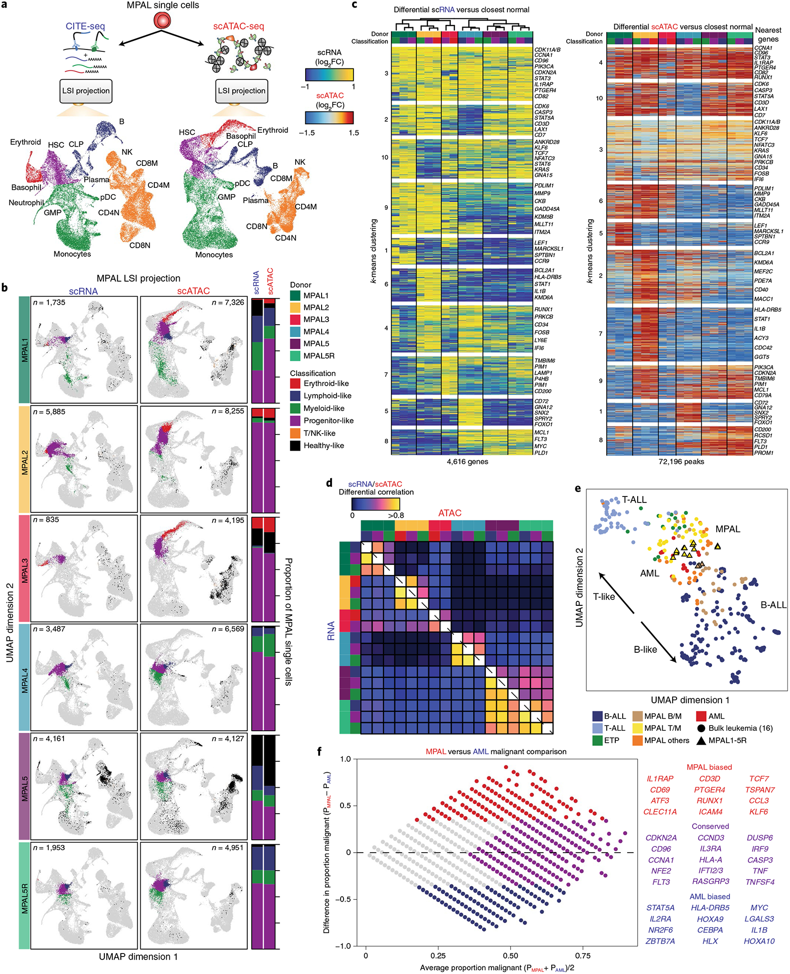
a, Schematic for projection of MPAL single cells onto hematopoiesis for both scRNA-seq and scATAC-seq classified into broad hematopoietic compartments. b, Left, MPAL single-cell projections into hematopoiesis for both scRNA-seq and scATAC-seq. Right, the proportion of MPAL cells that were broadly classified as healthy or disease and their respective hematopoietic compartment (range is from 0 to 1). c, Left, scRNA-seq heat map of upregulated genes (LFC >0.5 and two-sided t test FDR < 0.01) log₂(fold changes) comparing MPAL disease subpopulations to closest non-redundant normal cells. Differential genes were clustered using k-means clustering (k = 10) on the basis of their log₂(fold changes). Right, scATAC-seq heat map (ordered by scRNA-seq hierarchal clustering on the left) of differentially upregulated accessible peaks (LFC > 0.5 and two-sided t test FDR < 0.01) log₂(fold changes) comparing MPAL disease subpopulations to the closest non-redundant normal cells. Differential peaks were clustered using k-means clustering (k = 10) on the basis of their log₂(fold changes). d, Pearson correlation of the log₂(fold changes) (from c) for differentially upregulated genes and peaks across all MPAL subpopulations. e, LSI UMAP of differentially upregulated gene-expression profiles across bulk leukemias¹⁶ (circle, n = 321) and MPAL samples assayed in this study (outlined triangle, n = 17), colored by WHO 2016 classifications⁵. f, Left, MA plot (log-ratio (M) by mean average (A)) comparing the proportion of malignant (upregulated) gene-expression profiles in AML and MPALs. The x axis represents, for each upregulated gene, the average proportion of subpopulations from patients with AML and MPAL that are broadly upregulated (LFC > 0.5). The y axis represents, for each upregulated gene, the difference in the proportion of upregulated subpopulations from patients with MPAL and AML (LFC > 0.5). Right, genes that are more malignantly biased to either AMLs or MPALs and genes that are conserved across both AMLs and MPALs.

Using this LSI-projection framework and landscapes of healthy hematopoiesis, we next sought to deconvolve the normal and leukemic signatures of MPAL samples at a single-cell resolution. First, the leukemic single cells were projected into the hematopoietic linear LSI subspace. Next, we identified a non-redundant set of healthy hematopoietic cells that were nearest-neighbor normal cells to each leukemic cell, irrespective of their cell-type boundaries. Lastly, we computed the differences between the leukemic cells and nearest normal cells to identify the leukemic specific signature. We first tested our approach by analyzing recently published scRNA-seq data from samples from patients with acute myeloid leukemia (AML)¹⁹. By projecting the AMLs into our healthy hematopoietic map, we see general agreement with previous classifications without the need for potentially arbitrary cell-type boundaries on normal hematopoiesis (Supplementary Fig. 7a–c). We next wanted to classify our phenotypically diverse samples from patients with MPAL using our hematopoietic maps. First, we clustered our MPALs with our hematopoietic data to classify cells as ‘disease-like’ MPAL cells or ‘healthy-like’ cells (Supplementary Fig. 8a). These classifications generally agreed with the fraction of cells classified as blasts by morphology or flow cytometry (Supplementary Fig. 8b). We then projected our MPAL single cells onto our hematopoietic maps and discovered broad epigenetic and gene-expression diversity. To further resolve this diversity, we grouped MPAL cells within individual patients into broad hematopoietic developmental compartments: progenitor-like (comprising human stem cell and multipotent progenitor-like cells), lymphoid-like (comprising lymphoid-primed multipotent progenitors), erythroid-like (includes megakaryocyte-erythroid progenitors), myeloid-like (includes granulocyte-monocyte progenitors) and T/natural killer (NK)-like (includes differentiated T and NK cells²⁴) (Fig. 2a,b and Supplementary Fig. 8a). The scADT-seq data resolve the dominant subpopulations in the bilineal MPAL1 and MPAL5; however, it does not fully capture the transcriptional diversity in the other MPALs 2–4 (Supplementary Fig. 8c). We visualized these projected MPALs colored by these broad hematopoietic compartments, observing the expected high concordance between the scRNA-seq and scATAC-seq classifications (Fig. 2b). Comparing MPAL gene expression to this healthy nearest-neighbor set allowed the identification of pathogenic differential gene expression for MPALs from different compartments. In total, we identified 4,616 genes that were significantly upregulated (log₂ fold change (LFC) > 0.5 and false-discovery rate (FDR) < 0.01, see Supplementary Table 4) in at least one MPAL subpopulation across the six patient samples, and grouped these genes with k-means clustering (Fig. 2c). We further categorized the most conserved differential genes, TFs and KEGG pathways across the MPALs²⁵ (Supplementary Fig. 9a–c). Using the same approach for the scATAC-seq data, we performed testing of differential peaks for each MPAL subpopulation and found 72,196 significantly upregulated peaks (LFC > 0.5 and FDR < 0.05; Supplementary Table 4) in at least one MPAL subpopulation (Fig. 2c). Multiomic differential tracks for the cyclin-dependent kinase CDK11A and cyclin-dependent kinase inhibitor CDKN2A, genes that are recurrently mutated in MPAL^16,26, demonstrate these leukemia-specific ATAC-seq and RNA-seq differences (Supplementary Fig. 9d,e). Additionally, we calculated Pearson correlations of the differential genes and peaks and found that transcription and accessibility differs significantly across patients, but is relatively conserved across subpopulations within patients. (Fig. 2d).

To compare the leukemic programs of the MPAL hematopoietic compartments to previous studies, we downsampled bulk leukemia RNA-seq and projected onto our transcriptomic hematopoietic UMAP for childhood AMLs, B acute lymphoblastic leukemias (B-ALLs), early T cell precursor T acute lymphoblastic leukemias (ETP T-ALLs), non-ETP T-ALLs and MPALs¹⁶ (Supplementary Fig. 10a,b). We calculated differential expression with respect to the closest normal cell populations to identify their respective leukemic programs. Next, we performed LSI on variable malignant genes across all the leukemia subtypes, including MPAL1-MPAL5, and then visualized these patients with UMAP (Fig. 2e and Supplementary Fig. 10c,d). Interestingly, we found large differences in the leukemic programs across various leukemias including T-ALLs and B-ALLs, as well as across different cytogenetic subtypes. In addition, we found that the MPALs assayed in this study were representative of previously characterized MPALs¹⁶ (Fig. 2e). Given that we were insufficiently powered to detect unique leukemic differences between AML and our MPAL samples when analyzing downsampled bulk data, we compared the malignant transcriptomic profiles identified from reanalyzed AML scRNA-seq data¹⁸ with our MPALs to dissect further these unique malignant signatures (Fig. 2c and Supplementary Fig. 7c). To this end, we identified genes that were more commonly universally upregulated in AMLs or in MPALs, or jointly upregulated in both leukemias (Fig. 2f, Supplementary Fig. 7c and Supplementary Table 4). These gene sets provide fine-grained phenotypic resolution for comparing the differences and similarities between AML and MPAL leukemic programs and suggest possible insight into why MPALs respond poorly to AML treatment^27,28.

Having compared our leukemic transcriptomic programs to other studies we wanted to identify the key TFs that regulate these programs. First, we identified which TFs were differentially enriched in each k-means cluster of differentially accessible peaks observed in Fig. 2c (Fig. 3a and Supplementary Table 5). We found that RUNX1 motifs were highly enriched in both cluster 4 and 10—the two clusters corresponding to the most commonly shared accessible elements across MPAL subset populations. In addition, RUNX1 is significantly upregulated in about half (7 of 17) of the MPAL subpopulations. RUNX1 is one of the most frequently mutated genes across hematologic malignancies acting as both a tumor suppressor with loss-of-function mutations in AML²⁹, myelodysplastic syndrome³⁰ and ETP T-ALL^31,32, and as a putative oncogene in non-ETP T-ALL^33,34. Furthermore, wild-type RUNX1 has been implicated as a potential driver of leukemogenesis in core-binding factor leukemia³⁵ and mixed-lineage leukemia³⁶.

Fig. 3 |. Integrative scATAC-seq and scRNA-seq analyses nominate putative TFs that regulate leukemic programs.

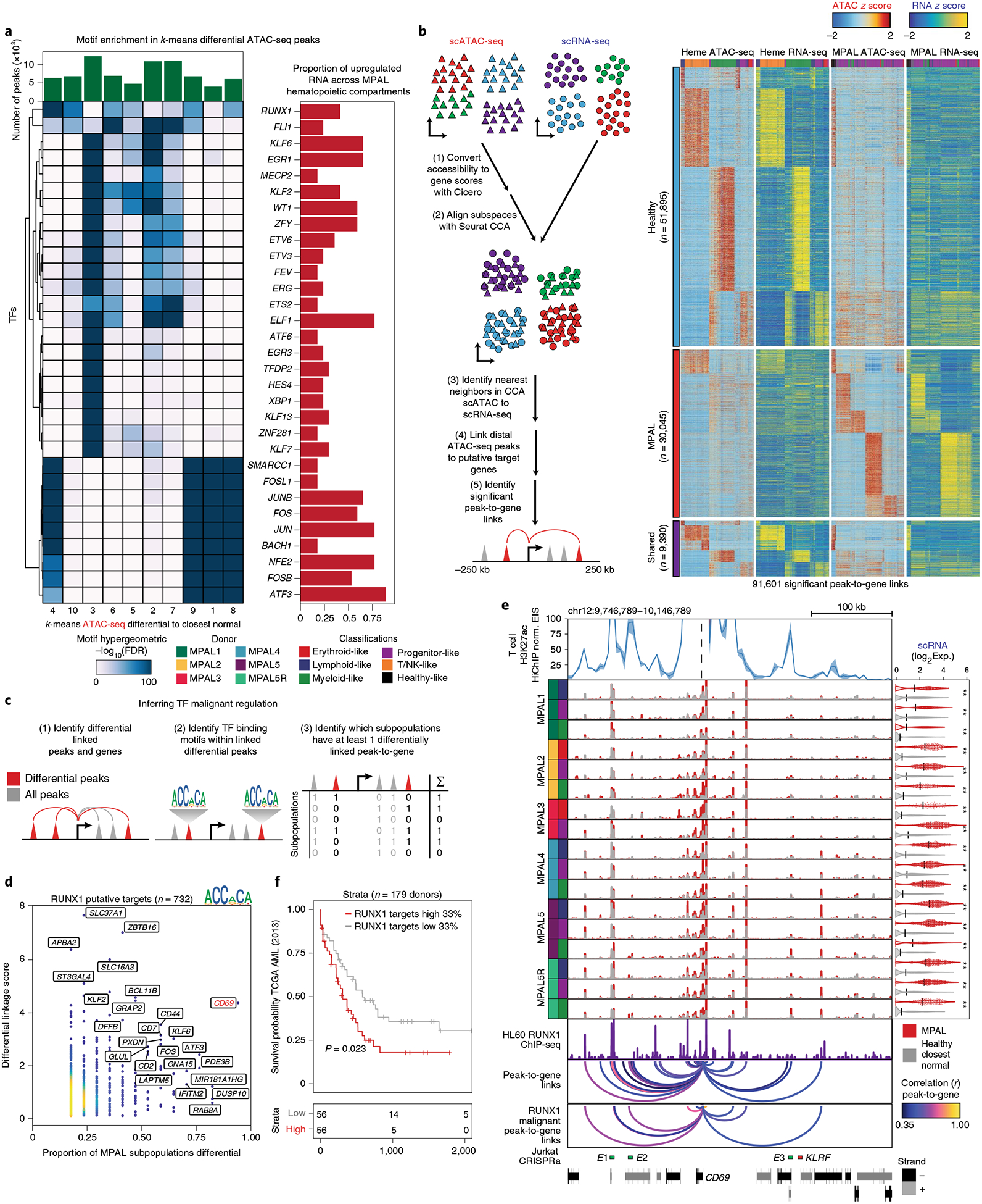
a, Top, number of accessible peaks in each k-means cluster. Bottom left, hypergeometric TF motif enrichment FDR in differentially accessible peaks across each k-means cluster identified in Fig. 2c. TFs are also identified as being differentially expressed and enriched in at least three MPAL hematopoietic compartments. Bottom right, proportion of differentially upregulated TF gene-expression profiles across MPAL hematopoietic compartments. b, Left, schematic for alignment of scATAC-seq and scRNA-seq data to link putative regulatory regions to target genes. First, scATAC-seq data are converted from accessible peaks to inferred gene-activity scores using Cicero. Second, these gene activity scores and scRNA-seq expression are aligned into a common subspace using Seurat’s CCA. Third, each scATAC-seq cell is assigned its nearest scRNA-seq neighbor. Fourth, ATAC-seq peaks within 2.5–250 kb of a gene promoter are correlated within the healthy hematopoietic and MPAL k-neaest-neighbor groupings. Lastly, significant peak-to-gene links are identified by correlating peaks to genes on different chromosomes. Right, heat maps of 91,601 peak-to-gene links across hematopoiesis and MPALs. Top, peak-to-gene links that are identified only within hematopoiesis. Middle, peak-to-gene links that are unique to MPALs. Bottom, peak-to-gene links identified in both hematopoiesis and MPALs. c, Schematic for identifying genes that are putatively regulated by the TF of interest. d, Putative RUNX1-target genes (n = 732) differentially upregulated in at least one MPAL subpopulation. The x axis represents the proportion of MPAL subpopulations that are differential in both scRNA-seq and a linked accessible peak. The y axis represents the cumulative linkage score between differentially upregulated peaks linked to differentially upregulated genes. e, CD69 multiomic differential track. Top, T cell T helper 17 H3K27ac HiChIP virtual 4C of enhancer interaction signal (EIS) of the CD69 locus, the line represents the average signal and shading represents the range of the signal times $\sqrt{2}$ between biological replicates (n = 2). Middle, aggregated scATAC-seq tracks showing MPAL disease subpopulations (red) and aggregated nearest-neighbor healthy (gray). Right, violin plots of the distribution log2 normalized expression of CD69 for MPAL disease subpopulations (red) and closest normal cells (gray); the black line represents the mean and asterisks denote significance (LFC > 0.5 and FDR < 0.01 from Fig. 2c). Violin plot of the log₂-normalized expression and the black line represents the mean log₂-normalized expression. Bottom, HL60 AML line ChIP-seq data across the CD69 locus, CD69 peak-to-gene links, RUNX1-identified malignant peak-to-gene links for CD69 and jurkat CRISPR activation of three CD69 enhancers³⁹ (E1-E3 are shown in green and the KLRF locus negative control is shown in red). Peak-to-gene links are colored by Pearson correlation of the peak accessibility and gene expression (Methods). f, Kaplan-Meier curve for patients with AML from TCGA (n = 179) stratified by putative RUNX1-target genes (n = 732); top 33% versus bottom 33%, average z score log₂(expression) (log-rank test P = 0.023).

To link RUNX1 and other putative regulatory TFs to their leukemic programs we first developed an analytical framework that utilizes both our transcriptomic and chromatin single-cell data to link putative regulator peaks to target genes. We used our matched scATAC-seq and scRNA-seq data for all MPALs and concordant hematopoietic maps, and aligned each cell into a common subspace using canonical correlation analyses (CCA)^10,11,37,38. For each scATAC-seq cell, we identified the nearest scRNA-seq neighbor (Fig. 3b and Supplementary Fig. 11a,b). We found that the mapping of scATAC-seq cell clusters to scRNA-defined cell clusters was highly consistent (single-cell overlap of 52% across 26 clusters; Supplementary Fig. 12a–d). We then aggregated our scATAC-seq cells on the basis of nearest neighbors in the LSI subspace using Cicero¹⁴ and created a corresponding scRNA-seq aggregate for each cluster using the constructed CCA alignment. We next identified 91,601 peak-to-gene links by correlating accessibility changes of ATAC peaks within 250 kb of the gene promoter with the expression of the gene independently for both healthy and MPAL aggregates (Fig. 3b and Supplementary Table 5). This analysis revealed peak-to-gene links that were specific to healthy hematopoiesis, others that were specific to MPALs and a conserved subset that was shared across both hematopoiesis and MPALs. We hypothesize that the MPAL-specific peak-to-gene links may be important for leukemic gene regulation. Overall, the identified set of peak-to-gene links had similar distributions for peaks mapped per gene, genes mapped per peak, number of skipped genes and the peak-to-gene as previously observed in a similar linkage analyses² (Supplementary Fig. 12e). To further support these peak-to-gene links, we used previously published H3K27ac HiChIP in primary T cells and a human coronary artery smooth muscle (HCASM) cell line and found that the T/NK-biased peak-to-gene links were more enriched in T cells than the HCASM cell line³⁹ (Supplementary Fig. 12f). We next examined GTEx expression quantitative trait locus (eQTL) mappings within our inferred peak-to-gene links, finding enrichment of eQTLs in several functionally related categories such as whole blood and lymphocytes (Supplementary Fig. 12g). To demonstrate the utility of these peak-to-gene links, we linked differentially accessible regions to known leukemic genes such as the surface protein CD96, the leukemic stem cell marker IL1RAP, the cytokine receptor FLT3 and apoptosis regulator MCL1 (Supplementary Fig. 13a–d). Overall, these analyses, show that the peak-to-gene links are highly enriched in immune regulation and across other previously published linkage datasets^2,39.

Having established a high-quality set of peak-to-gene links, we aimed to identify the set of malignant genes putatively regulated by RUNX1. First, we utilized our peak-to-gene links to identify differential peaks linked to a differential gene within at least two MPAL subpopulations. Next, we selected all linked differential accessibility sites that contain the RUNX1 motif. Finally, for each linked gene we combined all linked peaks to create a differential linkage score (Methods) and compared this score to the proportion of MPAL subpopulations that exhibited differential expression and accessibility in at least one linked peak and target gene (a measure of how common this RUNX1-driven dysfunction is across MPAL subsets) (Fig. 3c). Using this approach, we found 732 genes putatively regulated by a RUNX1-containing distal element in at least two MPAL subsets, and found that CD69, which is implicated in lymphocyte activation through initiation of JAK-STAT signaling⁴⁰ and lymphocyte retention in lymphoid organs⁴¹, was both highly enriched in the calculated differential linkage score and was observed to be differentially upregulated in almost every MPAL subpopulation (Fig. 3d and Supplementary Table 5). To further support the predicted RUNX1 regulation of CD69 (refs.^42,43), we incorporated T cell H3K27ac HiChIP³⁹, CRISPR-activation-validated CD69 enhancers^39,44 and RUNX1 ChIP-seq⁴⁵ into our multiomic differential track. These orthogonal datasets support RUNX1 binding to these linked distal regulatory regions (Fig. 3e). Finally, by using the 732 identified RUNX1-target genes to stratify patients with AML from The Cancer Genome Atlas (TCGA)⁴⁶ by expression, we observed significantly decreased survival (P = 0.023) in donors with a high RUNX1-target-gene signature⁴⁶ (Fig. 3f). This analysis suggests that RUNX1 is an important TF that putatively upregulates a portion of the leukemic signature in MPAL and potentially AML.

Collectively, this work establishes an experimental and analytical approach for deconstructing cancer-specific features using integrative analysis of multiple single-cell technologies. We find that MPAL malignant programs are largely conserved across phenotypically heterogenous cells within individual patients; this observation is consistent with a previous report¹⁶ that MPAL cells likely originate from a multipotent progenitor cell, thereby sharing a common mutational landscape while populating different regions of the hematopoietic tree. We used integrative single-cell analyses to further define putative TF regulation of these malignant programs. We inferred that RUNX1 acts as a potential oncogene in MPAL, regulating malignant genes associated with poor survival. We anticipate that similar approaches will be used in future studies to both identify the differentiation status of different tumor types (that is, identify the closest normal cell type) and enable molecular dissection of molecular dysfunction in pathogenic cellular subtypes, with the ultimate goal of identifying personalized therapeutic targets through integrative single-cell molecular characterization.

Methods

Experimental methods.

Description of healthy donors.

PBMCs, BMMCs and CD34⁺ bone marrow cells were obtained from healthy donors with informed consent and compliance with relevant ethical regulations (AllCells). Individual information for each donor is provided in Supplementary Table 1. All healthy cells used in this study were cryopreserved (fresh frozen in either Bambanker freezing medium or 10% DMSO with 90% serum). Thawed cells were not filtered for viability before loading into droplets. High-quality cells were identified bioinformatically.

Description of patients and donors with leukemia.

Patient samples were collected with informed consent in accordance with all relevant ethical regulations regarding human research participants under a protocol approved by the Institutional Review Board (IRB) at Stanford University Medical Center (Stanford IRB, 42949, 18329 and 6453). Peripheral blood and bone marrow aspirate samples were processed by Lymphoprep (STEMCELL Technologies) gradient centrifugation and fresh frozen in Bambanker medium. Diagnostic flow cytometry performed on bone marrow aspirate samples were analyzed. In all cases, a retrospective review of clinical parameters, hemogram data, peripheral blood smears, bone marrow aspirates, trephine biopsies, results of karyotype and flow cytometry studies was performed. Clinical follow-up information was obtained by retrospective review of the medical record charts. Cases were classified using the 2016 WHO classification of hematopoietic and lymphoid neoplasms⁵. Thawed cells were not filtered for viability before loading into droplet assays. High-quality cells were identified bioinformatically.

Combined single-cell antibody-derived tag and RNA sequencing.

CITE-seq was performed as previously reported⁶ using the (version 2) Chromium Single Cell 3′ Library and Gel Bead kit (10x Genomics, 120237). Six thousand cells were targeted for each sample. Oligonucleotide-coupled antibodies were obtained from Biolegend, indexed by PCR (ten cycles) with custom barcodes (see Supplementary Table 3), quantified by PCR using a PhiX Control v3 (Illumina, FC-110–3001) standard curve and sequenced on an Illumina NextSeq 550 together with scRNA-seq at no more than 60% of the total library composition (1.5 pM loading concentration, 26 × 8 × 0 × 98 base pair (bp) read configuration).

Single-cell assay for transposase-accessible chromatin using sequencing.

scATAC-seq targeting 4,000 cells per sample was performed using a beta version of Chromium Single Cell ATAC Library and Gel Bead kit (10x Genomics, 1000110). Each sample library was uniquely barcoded and quantified by PCR using a PhiX Control v3 (Illumina, FC-110–3001) standard curve. Libraries were then pooled and loaded on a NextSeq 550 Illumina sequencer (1.4 pM loading concentration, 33 × 8 × 16 × 33 bp read configuration) and sequenced to either 90% saturation or 30,000 unique reads per cell on average.

Whole-exome sequencing of patients and donors with leukemia.

Genomic DNA was extracted from diagnostic PBMCs or bone marrow samples using the Zymo Clean and Concentrator kit. Library construction (Agilent SureSelect Human All Exon kit), quality assessment and 150-bp paired-end sequencing (HiSeq4000) were performed by Novogene. Reads with adaptor contamination, uncertain nucleotides and paired reads with >50% low-quality nucleotides were discarded. Paired-end reads were then aligned to the reference genome (GRCh37) using BWA software. Genome Analysis Toolkit (GATK) was used to ignore duplicates with Picard-tool. Filtered variants (single-nucleotide polymorphisms and indels) were identified using GATK HaplotypeCaller and variantFiltration. Variants obtained from initial analysis were further compared to dbSNP and the 1,000 Genomes database. Finally, missense, stop-gain and frameshift mutations were compared against a custom panel of 300 genes that are recurrently mutated in hematologic malignancies as described previously^16,17.

Analytical methods.

Fluorescence-activated cell sorting.

Flow cytometry was performed on a FACSCalibur or FACSCanto II (Becton Dickinson) cytometer using commercially available antibodies (Supplementary Table 2). Lymphocytes were identified by low side scatter and bright CD45 expression. The gate was validated by backgating on CD3⁺ or CD19⁺ events. Blasts were identified by low side scatter and dim CD45 expression. The gate was further assessed by backgating on CD34⁺ events. Gates were drawn by additionally using isotype controls and internal positive and negative controls.

scADT-seq analysis.

Raw sequencing data were converted to fastq format using bcl2fastq (Illumina, v.2.20.0.422). ADTs were then assigned to individual cells and antibodies (see reference antibody barcodes in Supplementary Table 3) allowing for two and three barcode mismatches, respectively. Unique molecular counts for each cell and antibody were then generated by counting only barcodes with a unique molecular identifier (UMI). PBMC and BMMC ADT count data were transformed using the centered log ratio (CLR) as previously described⁶. PBMCs and BMMCs were visualized in two dimensions using the uwot implementation of UMAP¹² in R (n_neighbors = 50, min_dist = 0.4).

scATAC-seq.

scATAC-seq processing.

Raw sequencing data were converted to fastq format using cellranger atac mkfastq (10x Genomics, v.1.0.0; Supplementary Fig. 14). scRNA-seq reads were aligned to the GRCh37 (hg19) reference genome and quantified using cellranger count (10x Genomics, v.1.0.0).

scATAC-seq quality control.

To ensure that each cell was both adequately sequenced and had a high signal-to-background ratio, we filtered cells with less than 1,000 unique fragments and enrichment at TSSs below 8. To calculate TSS enrichment², genome-wide Tn5-corrected insertions were aggregated ±2,000 bp relative (TSS-strand-corrected) to each unique TSS. This profile was normalized to the mean accessibility ±1,900–2,000 bp from the TSS, smoothed every 51 bp and the maximum smoothed value was reported as TSS enrichment in R. We estimate that the multiplet percentage for this study was around 4% (ref.⁷).

scATAC-seq counts matrix.

To construct a counts matrix for each cell by each feature (window or peaks), we read each fragment.tsv.gz fill into a GenomicRanges object. For each Tn5 insertion, which can be thought of as the ‘start’ and ‘end’ of the ATAC fragments, we used findOverlaps to find all overlaps with the feature by insertions. Then we added a column with the unique id (integer) cell barcode to the overlaps object and fed this into a sparseMatrix in R. To calculate the fraction of reads/insertions in peaks, we used the colSums of the sparseMatrix and divided it by the number of insertions for each cell id barcode using table in R.

scATAC-seq union peak set from latent semantic index clustering.

We adapted a previous workflow for generating a union peak set that will account for diverse subpopulation structure^2,9,10 (Supplementary Fig. 14). First, we created 2.5-kb windows genome wide using ‘tile(hg19chromSizes, width = 2500)’ in R. Next, a cell-by-2.5-kb-window sparse matrix was constructed as described above. The top 20,000 accessible windows were kept and the binarized matrix was transformed with the term frequency-inverse document frequency (TF-IDF) transformation⁸. In brief, we divided each index by the colSums of the matrix to compute the cell ‘term frequency’. Next, we multiplied these values by log(1 + ncol(matrix)/rowSums(matrix)), which represents the ‘inverse document frequency’. This normalization resulted in a TF-IDF matrix that was then used as input to the irlba singular value decomposition (SVD) implementation in R. The 2nd to 25th SVD dimensions (1st dimension is correlated with the depth of cell reads¹⁵) were used for creating a Seurat object and initial clustering was performed using Seurat’s SNN graph clustering (v.2.3.4) with ‘FindClusters’ at a default resolution of 0.8. If the minimum cluster size was below 200 cells, the resolution was decreased until this criterion was reached leading to a final resolution of 0.8^N (where N represents the iterations until the minimum cluster size is 200 cells). For each cluster, peak calling was performed on Tn5-corrected insertions (each end of the Tn5-corrected fragments) using the MACS2 callpeak command with parameters ‘--shift −75 --extsize 150 --nomodel --call-summits --nolambda --keep-dup all -q 0.05’. The peak summits were then extended by 250 bp on either side to a final width of 501 bp, filtered by the ENCODE hg19 blacklist (https://www.encodeproject.org/annotations/ENCSR636HFF/) and filtered to remove peaks that extend beyond the ends of chromosomes.

Overlapping peaks called were handled using an iterative removal procedure as previously described². First, the most significant (MACS2 score) extended peak summit is kept and any peak that directly overlaps with that significant peak is removed. This process reiterates to the next most significant peak until all peaks have either been kept or removed owing to direct overlap with a more significant peak. The most significant 200,000 extended peak summits for each cluster were quantile normalized using ‘trunc(rank(v))/length(v)’ in R (where v represents the vector of MACS2 peaks scores). These cluster peak sets were then merged and the previous iterative removal procedure was used. Lastly, we removed any peaks whose nucleotide content had any ‘N’ nucleotides and any peaks mapping to chrY.

scATAC-seq-centric latent semantic indexing clustering and visualization.

scATAC-seq clustering was performed by adapting the strategy of Cusanovich et. al^9,10 to compute the term TF-IDF transformation. In brief, we divided each index by the colSums of the matrix to compute the cell ‘term frequency’. Next, we multiplied these values by log(1 + ncol(matrix)/rowSums(matrix)), which represents the ‘inverse document frequency’. This resulted in a TF-IDF matrix that was used as input to the irlba SVD implementation in R. The first 50 SVD dimensions were used as input into a Seurat object and initial clustering was performed using Seurat’s (v.2.3.4) SNN graph clustering ‘FindClusters’ with a resolution of 1.5 (25 SVD dimensions for healthy hematopoiesis and 50 for healthy hematopoiesis and MPALs). We found that in some cases, there was batch effect between experiments. To minimize this effect, we identified the top 50,000 variable peaks across the initial clusters (summed cell matrix for each cluster followed by edgeR log(counts per million) (CPM) transformation⁴⁷). These 50,000 variable peaks were then used to subset the sparse binarized accessibility matrix and recompute the TF-IDF transform. We used SVD on the TF-IDF matrix to generate a lower-dimensional representation of the data by retaining the first 50 dimensions. We then used these reduced dimensions as input into a Seurat object and then final clusters were identified by using Seurat’s (v.2.3.4) SNN graph clustering ‘FindClusters’ with a resolution of 1.5 (50 SVD dimensions for healthy hematopoiesis and 50 for healthy hematopoiesis and MPALs). These same reduced dimensions were used as input to the uwot implementation of UMAP (n_neighbors = 55, n_components = 2, min_dist = 0.45) and plotted in ggplot2 using R. We merged scATAC-seq clusters from a total of 36 clusters for hematopoiesis to 26 final clusters that best agreed with the scRNA-seq clusters. The objective of this analysis is to optimize feature selection, which minimizes batch effects, and enable projection of future data into the same manifold as described further below.

scATAC-seq visualization in genomic regions.

To visualize scATAC-seq data, we read the fragments into a GenomicRanges object in R. We then computed sliding windows across each region we wanted to visualize every 100 bp ‘slidingWindow s(region,100,100)’. We computed a counts matrix for Tn5-corrected insertions as described above and then binarized this matrix. We then returned all non-zero indices (binarization) from the matrix (cell × 100-bp intervals) and plotted them in ggplot2 in R with ‘geom_tile’. For visualizing aggregate scATAC-seq data, the binarized matrix above was summed and normalized. Scale factors were computed by taking the binarized sum in the global peak set and normalizing to 10,000,000. Tracks were then plotted in ggplot in R.

chromVAR.

We measured global TF activity using chromVAR¹⁵. We used the cell-by-peaks and the Catalog of Inferred Sequence Binding Preferences (CIS-BP) motif (from chromVAR motifs ‘human_pwms_v1’) matches within these peaks from motifmatchr. We then computed the GC-bias-corrected deviations using the chromVAR ‘deviations’ function. We then computed the GC-bias-corrected deviation scores using the chromVAR ‘deviationScores’ function.

Gene-activity scores using Cicero and co-accessibility.

We calculated gene activities using the R package Cicero¹⁴. In brief, we used the sparse binary cell-by-peaks matrix and created a cellDataSet, detectedGenes and estimatedSizeFactors. We then created a ‘cicero_cds’ with k = 50 and the ‘reduced_coordinates’ being the LSI SVD coordinates (hematopoiesis = 25, hematopoiesis and MPALs = 50). This function returns aggregated accessibility across groupings of cells on the basis of nearest-neighbor rules from the R package FNN. We then identified all peak-peak linkages that were within 250 kb by resizing the peaks to 250 kb and 1 bp and using ‘findOverlaps’ in R. We calculated the Pearson correlation for each unique peak-peak link and created a connections data.frame where the first column is peak_i, the second column is peak_j and the third column is co-accessibility (Pearson correlation). We created a gene data.frame from the TxDb ‘TxDb.Hsapiens.UCSC. hg19.knownGene’ in R, resized each gene from its TSS and created a window ±2.5 kb centered at the TSS and annotated the ‘cicero_cds’ using ‘annotate_cds_by_site’. We then calculated gene activities with ‘build_gene_activity_matrix’ (co-access cutoff of 0.35). Lastly we normalized the gene activities by using ‘normalize_gene_activities’ and the read depth of the cells, log normalized these gene activities scores for interpretability by computing log₂(GA × 1,000,000 + 1), where GA is the gene activity score.

scRNA-seq.

scRNA-seq processing.

Raw sequencing data were converted to fastq format using cellranger mkfastq (10x Genomics, v.3.0.0; Supplementary Fig. 14). scRNA-seq reads were aligned to the GRCh37 (hg19) reference genome and quantified using cellranger count (10x Genomics, v.3.0.0). We kept genes that were present in both 10x gene transfer formatfiles v.3.0.0 for hg19 and hg38 (https://support.10xgenomics.com/single-cell-gene-expression/software/release-notes/build). Mitochondrial and ribosomal genes were also filtered before further analysis. Genes remaining after these filtering steps we refer to as ‘informative’ genes and enable cross genome comparison.

scRNA-seq quality control.

We wanted to filter out cells whose transcripts were lowly captured and first plotted the distribution of genes detected and UMIs for all experiments. On the basis of these plots, we chose to filter out cells that had less than 400 informative genes detected and 1,000 UMIs. In addition, to lower multiplet representation, we filtered cells with above 10,000 UMIs. We estimate that the multiplet percentage for this study was around 6% (ref.⁸). We then plotted the correlation for each replicate experiment and found high reproducibility.

scRNA-seq-centric latent semantic indexing clustering and visualization.

We initially tested a few methods for clustering scRNA-seq but settled on an approach that enabled us to effectively capture the hematopoietic hierarchy without substantial alteration of transcript expression (Supplementary Fig. 14). We first log normalized the transcript counts by first depth normalizing to 10,000 and adding a pseudocount before a log₂ transform (log₂(counts per ten thousand transcripts + 1)). Next, we identified the top 3,000 variable genes and performed the TF-IDF transform on these 3,000 genes. We performed SVD on this transformed matrix keeping the first 25 dimensions and used this as input to Seurat’s SNN clustering (v.2.3.4) with an initial resolution of 0.2. We summed the individual clusters single cells and computed the logCPM transformation, ‘edgeR::cpm(mat,log = TRUE,prior.count = 3)’, and identified the top 2,500 variable genes across these initial clusters. These variable genes were used as input for a TF-IDF transform and an SVD was performed on this transformed matrix keeping the first 25 dimensions, which were used as input to Seurat’s SNN clustering (v.2.3.4) with an increased resolution of 0.6. We then summed the individual clusters single cells, computed the logCPM transformation, ‘edgeR::cpm(mat,log = TRUE,prior.count = 3)’ and identified the top 2,500 variable genes across these clusters. We repeated this one more time (resolution 1.0) and saved the final features and clusters. To align our clusters better with the scATAC-seq data, we merged a total of 26 clusters from 31 initial clusters (included in Supplemental Data). These LSI dimensions were used as input to the uwot implementation of UMAP (n_neighbors = 35, n_components = 2, min_dist = 0.45) and plotted in ggplot2 using R. The objective of this analysis is to optimize feature selection, which minimizes batch effects, and enable projection of future data into the same manifold as described further below.

scATAC-seq and scRNA-seq analytical methods.

Latent semantic indexing projection for scATAC-seq and scRNA-seq.

We designed the above analytical approach to clustering of single-cell data because it optimized feature selection and enabled projection of new non-normalized data into a low-dimension manifold. To enable these analyses, when computing the TF-IDF transformation on the hematopoietic hierarchy, we kept the colSums, rowSums and SVD from the previous run and then when projecting new data into this subspace, we first identified which row indices to zero out on the basis of the initial TF-IDF rowSums. We then computed the ‘term frequency’ by dividing by the colSums in these features. Next, we computed the ‘inverse document frequency’ from the previous TF-IDF transform (diagonal(1 + ncol(mat)/rowSums(mat))) and computed the new TF-IDF transform. We projected this TF-IDF matrix into the SVD subspace that was previously generated. To do this calculation, we computed the new coordinates by “t(TF_IDF) %*% SVD$u %*% diag(1/SVD$d)”, where TF_IDF is the transformed matrix and SVD is the previous SVD run, using irlba in R (v.3.5.1). We computed the projected matrix by “SVD$u %*% diag(SVD$D) * t(V)” where V is the projected coordinates above. For projecting bulk RNA-seq, we downsampled previously published data to 5,000 reads in genes 100 times and then made a sparse matrix for projection as single-cell data. For projecting bulk scATAC-seq, we downsampled previously published data to 10,000 reads in peaks 100 times and then made a binary sparse matrix for projection as single-cell data.

HCA immune census bone marrow projection.

We downloaded the HCA bone marrow immune census data (https://data.humancellatlas.org/explore/projects/cc95ff89-2e68-4a08-a234-480eca21ce79)²³ comprising around 300,000 cells from eight different donors (filtered for at least 1000 UMI). We used our iterative LSI approach (resolutions = 0.2, 0.6, 1.0 and 2,500 variable genes; UMAP n_neighbors = 75, min_dist = 0.2, metric = “euclidean”) to create a UMAP manifold that we could then project our scRNA-seq data onto. We LSI projected our scRNA-seq data onto this subspace and found that our cohort reasonably repopulates the hematopoietic manifold created on completely separate donors. This result shows that our analysis approach is scalable and that our healthy hematopoietic data reasonably recapitulates the biological diversity along hematopoiesis.

Classification of AML scRNA-seq.

We wanted to evaluate our LSI projection of abnormal cells into a healthy subspace by using data from van Galen et al.¹⁹. We first projected their healthy bone marrow scRNA-seq from a different platform and genome and found remarkable agreement with their classifications and our independent hematopoietic manifold. We then projected their ‘disease’ cell AML scRNA-seq into our manifold and found reasonable agreement for more terminal states and less agreement in the ‘hematopoietic stem cell (HSC)’ and ‘progenitor-like’ classifications. We reasoned that this difference could be due to defining discrete populations in a continuous subspace. We then reclassified their AML ‘disease’ scRNA-seq by finding the nearest neighbors between their cells in our projected SVD subspace and our scRNA-seq data. We grouped our clusters into more broad groupings for interpretability (‘Progenitor-like’ is clusters 1–6, ‘GMP-like’ is clusters 7 and 8, ‘cDC-like’ is cluster 10, ‘Monocyte-like’ is clusters 11–13). For differential analyses we compared against their projected scRNA-seq healthy bone marrow to minimize batch differences in the comparison.

Classification of MPAL single cells with scATAC-seq and scRNA-seq.

We wanted to classify MPAL single cells on the basis of their disease state and hematopoietic progression. First, we aimed to determine which cells were healthy-like and disease-like. To do this analysis, we clustered all of the healthy hematopoietic cells with the MPAL of interest using our LSI workflow as described above (scRNA, 25 principal components (PCs), 1,000 variable genes, and Seurat’s SNN resolution of 0.2, 0.8 and 0.8; scATAC, 25 PCs, 25,000 variable peaks and Seurat’s SNN resolution of 0.8 and 0.8). We then defined clusters to be healthy-like if a high percentage (>80% for scRNA-seq and >90% for scATAC) of the cells were from the normal hematopoietic data. MPAL single cells belonging to these clusters were classified as healthy-like and the remaining cells were classified as disease-like. We note that we did not detect significant copy-number amplifications with scATAC-seq using a previously described approach⁷, and the proportion of cells classified as disease-like was consistent with flow cytometry and morphological estimations of the percentage of blast cells (Supplementary Fig. 8b). To accurately characterize these MPAL as disease-like by their hematopoietic state, we established ‘hematopoietic compartments’ across our scRNA-seq and scATAC-seq maps that broadly characterized the hematopoietic continuum. The borders for these compartments were determined empirically using ‘fhs’ in R, guided by the initial clusters and agreement across the scRNA-seq and scATAC-seq classifications. After classifying the normal hematopoietic continuum, we then broadly classified the MPAL disease-like cells on the basis of their projected nearest neighbor in the UMAP subspace. These classifications were used subsequently in differential analyses. We note that this approach identifies a cumulative set of leukemia-specific changes relative to similar hematopoietic cells and does not discriminate among intermediate changes along a leukemic developmental trajectory. We note that this method of classification is potentially limited as compared to classification on the basis common structural variants or mutations. Furthermore, identifying disease cells that are partially transformed may likewise be challenging.

Identifying differential features with scATAC-seq and scRNA-seq.

To identify differential features for previously published AML data and MPALs, we constructed a nearest-neighbor healthy aggregate using the following approach. First, we used FNN to identify the nearest 25 cells using ‘get.knnx(svdHealthy, svdProjected, k = 25)’ on the basis of Euclidean distance between the projected cells and hematopoietic cells in LSI SVD space. For each projected population, we used a minimum of 50 and maximum of 500 cells (random sampling) as input. Next, we took the unique of all hematopoietic single cells and if this number was greater than 1.25 times the number of the projected populations, we took the nearest 24 cells and repeated this procedure until this criterion was met. Then the projected population and non-redundant hematopoietic cells were downsampled to an equal number of cells (maximum 500). For scATAC-seq, we binarized the matrix for both the projected populations and hematopoietic matrices. Next, we scaled the sparse matrices to 10,000 total counts for scRNA-seq and 5,000 total promoter counts for scATAC-seq (promoter peaks defined as peaks within 500 bp of TSS from hg19 10x v.3.0.0 gene transfer format file). Next, we computed row-wise two-sided t tests for each feature. We then calculated the FDR using p.adjust(method = “fdr”). We then computed the log₂mean and log₂(fold changes) for each feature. We chose these parameters on the basis of a previous study comparing analytical methods for differential expression⁴⁸. For scRNA-seq, differential expression was determined by FDR < 0.01 and absolute log₂(fold changes) greater than 0.5. For scRNA-seq, differential expression was determined by FDR < 0.05 and absolute log₂(fold changes) greater than 0.05.

To identify differential genes for bulk leukemia RNA-seq, we downsampled the gene counts to 10,000 counts randomly for 250 times. We then projected and used the above framework to resolve differential genes with log₂(fold change) > 3 and FDR < 0.01. We then removed genes that were differential in 33% or higher of the normal samples to attempt to capture biased genes. In addition, we removed genes differential in 50% or higher of the leukemia samples. This filtering biases our identified malignant genes to those that are variable across the leukemic types as opposed to conserved across all leukemic types. We then took the average malignancy for each remaining gene for each leukemic type and used the top 300 variable malignant genes across the leukemic types for the heat map and LSI. For computing differential LSI, we binarized each gene as malignant or not for the 300 variable malignant genes and computed the TF-IDF transform followed by SVD (LSI). We then visualized this in two dimensions using the uwot implementation of UMAP (50 SVD dimensions, n_neighbors = 50, min_dist = 0.005).

Matching scATAC-seq-scRNA-seq pairs using Seurat’s canonical correlation analyses.

To integrate our epigenetic and transcriptomic data we built on previous approaches for integration^10,37. We found the approach that worked best for our integrative analyses was using Seurat’s CCA. We performed integration for each biological group separately because (1) it improved alignment accuracy and (2) required much less memory. First, for both the gene-activity scores matrix and scRNA-seq matrix, a Seurat object was created using ‘CreateSeuratObject’, normalized with ‘NormalizeData’ and the top 2,000 most variable genes or activities ranked by dispersion with ‘FindVariableGenes’ were. We defined the union of the top 2,000 most variable genes from scRNA-seq and gene scores from scATAC-seq and found this increased the concordance downstream (as defined by cluster-to-cluster mapping in hematopoiesis and single-cell Spearman correlations). These genes were then used for running CCA using ‘RunCCA’ with the number of canonical correlations to compute as 25. We then calculated the explained variance using ‘CalcVarExpRatio’ grouping by each of the individual experimental protocols scATAC-seq (gene-activity scores) and scRNA-seq. We then filtered cells where the variance explained by CCA was less than twofold as compared to principal component analysis. We aligned the subspaces with “AlignSubspace” and 25 dimensions to align with reduction.type = “cca” and grouping.var = “protocol”. For each scATAC-seq cell the nearest scRNA-seq cell was identified on the basis of minimizing the Euclidean distance. We created a UMAP using the aligned CCA coordinates as input into the uwot UMAP implementation with n_neighbors = 50, min_dist = 0.5, metric = “euclidean” and plotted the output with ggplot2 in R. To enable more robust correlation-based downstream analyses, we used our initial k-nearest-neighbor groupings (nGroups = 4998, KNN = 50) from Cicero¹⁴ to group scATAC-seq accessibility, gene-activity scores, scRNA-seq closest neighbor and chromVAR¹⁵ deviation scores.

Peak-to-gene linkage.

Cicero¹⁴ allows us to infer gene-activity scores by linking distally correlated ATAC peaks to the promoter peak. While this measure is extremely useful, it does not actually mean it is correlated to gene expression. To circumvent this limitation, we used our grouped scATAC-seq and grouped linked scRNA-seq to identify peak-to-gene links. First we log normalized the accessibility and gene expression with log₂(counts per 10,000 + 1) and then we resized each of the gene GenomicRanges to the start using resize(gr,1,“start”) and then resizing the start to a ±250-kb window using ‘resize(gr, 2 * 250000 + 1, “center”)’. We then overlapped all ATAC-seq peaks using ‘findOverlaps’ to identify all putative peak-to-gene links. We then split the aggregated ATAC and RNA matrices by whether the majority of the cells were from MPAL or hematopoietic single cells and correlated the peaks and genes for all putative peak-to-gene links. We used a previously described approach for computing a null correlation on the basis of trans correlations (correlating peaks and genes not on the same chromosome)². In brief, for each chromosome, 1,000 peaks not on the same chromosome are identified and correlated to every gene on that chromosome. Each putative peak-to-gene correlation is converted into a z score by using the mean and s.d. of the null trans correlations. These are then converted to P values and adjusted for multiple-hypothesis testing using the Benjamini-Hochberg correction ‘p.adjust’ in R. We retained links whose correlation (Pearson) was above 0.35 and FDR < 0.1 (the same correlation cutoff as co-accessibility in Cicero¹⁴) in either MPAL or hematopoietic aggregations. We then kept all peak-to-gene links that were greater than 2.5 kb in distance. We identified peak-to-gene links that are only present in hematopoiesis, MPALs or both. To visualize the peak-to-gene links we plotted all of them as a heat map with ComplexHeatmap. To determine the column order we first computed principal component analysis for the first 25 principal components using irlba. We computed Seurat¹¹ SNN clustering with a resolution of 1 and computed the cluster means. We then computed the order of these clusters using hclust and the dissimilarity 1 − R as the distance. Next, we iterated through each cluster and performed hclust with the dissimilarity calculations to get a final column order. The peak-to-gene links were grouped by k-means clustering with 10 input centers, 100 iterations and 10 random starts for healthy, disease and the overlapping links. We did this biclustering because it enabled us to plot smaller rasterized chunks of the heat map without overwhelming the memory; individual rasterized k-means clusters were put together after analysis.

Enrichment of peak-to-gene links in GTEx eQTLs.

We adopted a previous approach for identifying the enrichment of our peak-to-gene links in GTEx eQTL data. In brief, we downloaded GTEx eQTL data (version 7) from https://gtexportal.org/home/datasets and the *.signif_variant_gene_pairs.txt.gz files were used. We also downloaded gencode v19 (matched to these eQTLs) and identified all gene starts and the nearest gene starts to each peak and eQTL using ‘distanceToNearest. We filtered all eQTLs that were further than 250 kb from their predicted gene to be consistent with our linkage approach. To calculate a conservative overlap enrichment, we further pruned all eQTL links that were to its nearest gene. We then created a null set (n = 250) of peak-to-gene links by randomly selecting distal ATAC-seq peak-to-gene links (within 250 kb) that were distance matched to the links tested at a resolution of 5 kb. We then calculated a z score and enrichment for each peak-to-gene link set as compared to the null set and calculated an FDR using ‘p.adjust(method = “fdr”)’.

Enrichment of peak-to-gene links in K27ac HiChIP metaV4C.

We wanted to determine the specificity of our peak-to-gene links in published chromatin conformation data. We downloaded previously published naive T cell and HCASM cell line H3K27ac HiChIP data. We then identified within each peak-to-gene link subset the peaks that were most biased to T/NK cells. To do this analysis, we calculated the z score for each peak in the peak-to-gene links, removed all links below 100 kb and floored each peak coordinate (start or end) to its nearest 10-kb window. We then ranked these links by the z score for the peak, deduplicated the links at a resolution of 10 kb and kept the top 500 remaining peak-to-gene links. Next, we used juicer dump (no normalization “NONE”) at a 10-kb resolution for each chromosome in the ‘.hic’ file. We read each chromosome into an individual ‘sparseMatrix’ in R and scaled the sparse matrices such that the total cis interactions summed up to 10 million paired-end tags (PETs). Then, for each peak-to-gene link, the upstream or downstream window (column or row) (whether the peak was upstream or downstream of the gene promoter) was identified. To scale the distance of each interaction for interpretability, we linearly interpolated the data to be on a scale from −50% to 150% to visualize the focal interaction. The mean interaction signal was reported and repeated for both replicates. The mean and s.d. across both replicates were calculated and plotted with ggplot in R.

Identifying TF malignant target genes and survival analysis.

We wanted to create a framework for identifying TFs that potentially directly regulate malignant genes. To do this analysis, we first identified a set of TFs whose hypergeometric enrichment in differential peaks were high across the MPAL subpopulations (comparing upregulated peaks against all peaks) and that were identified as being transcriptionally correlated with the accessibility of their motif (see above). Next, for a given TF and all identified peak-to-gene links, we further subsetted these links by those containing the TF motif. For each MPAL subpopulation, we determined whether, for each peak-to-gene link, both the peak and gene were upregulated. Then for each gene, we gave a binary score indicating whether or not that MPAL subpopulation had at least one differential peak-to-gene link (whose peak and gene are differentially upregulated), and reported the proportion of subpopulations that were upregulated. In addition, for each gene that has at least one differential peak-to-gene link we summed their squared correlation R² and reported that as the differential linkage score. We kept all genes that had least one MPAL subpopulation with corresponding differential peak-to-gene links.

For survival analysis, we downloaded the RPKM TCGA-LAML data⁴⁶ (https://gdc.cancer.gov/about-data/publications/#/?groups=TCGA-LAML&years=&order=desc). We downloaded the survival data from Bioconductor RTCGA.clinical (“patient.vital_status”) and matched the RPKM expression using TCGA IDs. Next, we took all genes that were identified as target genes for RUNX1 (n = 732), and computed row-wise z scores for each gene. Next, we took the column means of this matrix to get an average z score across all RUNX1-target genes. We then identified the top 33% and bottom 33% of donors on the basis of this expression. We computed the P value using the R package survival ‘survfit(Surv(times,patient.vital_status)~Runx1_TG_Expression, LAML_Survival)’. We plotted the Kaplan-Meier curve using the R package survminer ‘ggsurvplot’ in R.

References

- 1.Hoadley KA et al. Cell-of-origin patterns dominate the molecular classification of 10,000 tumors from 33 types of cancer. Cell 173, 291–304 (2018). [DOI] [PMC free article] [PubMed] [Google Scholar]
- 2.Corces MR et al. The chromatin accessibility landscape of primary human cancers. Science 362, eaav1898 (2018). [DOI] [PMC free article] [PubMed] [Google Scholar]
- 3.Polak P et al. Cell-of-origin chromatin organization shapes the mutational landscape of cancer. Nature 518, 360–364 (2015). [DOI] [PMC free article] [PubMed] [Google Scholar]
- 4.Weinberg OK & Arber DA Mixed-phenotype acute leukemia: historical overview and a new definition. Leukemia 24, 1844–1851 (2010). [DOI] [PubMed] [Google Scholar]
- 5.Arber DA et al. The 2016 revision to the World Health Organization classification of myeloid neoplasms and acute leukemia. Blood 127, 2391–2405 (2016). [DOI] [PubMed] [Google Scholar]
- 6.Stoeckius M et al. Simultaneous epitope and transcriptome measurement in single cells. Nat. Methods 14, 865–868 (2017). [DOI] [PMC free article] [PubMed] [Google Scholar]
- 7.Satpathy AT et al. Massively parallel single-cell chromatin landscapes of human immune cell development and intratumoral T cell exhaustion. Nat. Biotechnol 37, 925–936 (2019). [DOI] [PMC free article] [PubMed] [Google Scholar]
- 8.Zheng GXY et al. Massively parallel digital transcriptional profiling of single cells. Nat. Commun 8, 14049 (2017). [DOI] [PMC free article] [PubMed] [Google Scholar]
- 9.Cusanovich DA et al. The cis-regulatory dynamics of embryonic development at single-cell resolution. Nature 555, 538–542 (2018). [DOI] [PMC free article] [PubMed] [Google Scholar]
- 10.Cusanovich DA et al. A single-cell atlas of in vivo mammalian chromatin accessibility. Cell 174, 1309–1324 (2018). [DOI] [PMC free article] [PubMed] [Google Scholar]
- 11.Butler A, Hoffman P, Smibert P, Papalexi E & Satija R Integrating single-cell transcriptomic data across different conditions, technologies, and species. Nat. Biotechnol 36, 411–420 (2018). [DOI] [PMC free article] [PubMed] [Google Scholar]
- 12.McInnes L, Healy J & Melville J UMAP: Uniform manifold approximation and projection for dimension reduction. Preprint at arXiv https://arxiv.org/abs/1802.03426 (2018). [Google Scholar]
- 13.Janeway CJ, Travers P, Walport M & Shlomchik MJ Immunobiology 5th edn (Garland Science, 2001). [Google Scholar]
- 14.Pliner HA et al. Cicero predicts cis-regulatory DNA interactions from single-cell chromatin accessibility data. Mol. Cell 71, 858–871 (2018). [DOI] [PMC free article] [PubMed] [Google Scholar]
- 15.Schep AN, Wu B, Buenrostro JD & Greenleaf WJ chromVAR: inferring transcription-factor-associated accessibility from single-cell epigenomic data. Nat. Methods 14, 975–978 (2017). [DOI] [PMC free article] [PubMed] [Google Scholar]
- 16.Alexander TB et al. The genetic basis and cell of origin of mixed phenotype acute leukaemia. Nature 562, 373–379 (2018). [DOI] [PMC free article] [PubMed] [Google Scholar]
- 17.Takahashi K et al. Integrative genomic analysis of adult mixed phenotype acute leukemia delineates lineage associated molecular subtypes. Nat. Commun 9, 2670 (2018). [DOI] [PMC free article] [PubMed] [Google Scholar]
- 18.Corces MR et al. Lineage-specific and single-cell chromatin accessibility charts human hematopoiesis and leukemia evolution. Nat. Genet 48, 1193–1203 (2016). [DOI] [PMC free article] [PubMed] [Google Scholar]
- 19.van Galen P et al. Single-cell RNA-seq reveals AML hierarchies relevant to disease progression and immunity. Cell 176, 1265–1281 (2019). [DOI] [PMC free article] [PubMed] [Google Scholar]
- 20.Satpathy AT et al. Transcript-indexed ATAC-seq for precision immune profiling. Nat. Med 24, 580–590 (2018). [DOI] [PMC free article] [PubMed] [Google Scholar]
- 21.Mezger A et al. High-throughput chromatin accessibility profiling at single-cell resolution. Nat. Commun 9, 3647 (2018). [DOI] [PMC free article] [PubMed] [Google Scholar]
- 22.Buenrostro JD et al. Integrated single-cell analysis maps the continuous regulatory landscape of human hematopoietic differentiation. Cell 173, 1535–1548 (2018). [DOI] [PMC free article] [PubMed] [Google Scholar]
- 23.Li B et al. Census of immune cells. HCA https://data.humancellatlas.org/explore/projects/cc95ff89-2e68-4a08-a234-480eca21ce79 (2018). [Google Scholar]
- 24.Mitchell K et al. IL1RAP potentiates multiple oncogenic signaling pathways in AML. J. Exp. Med 215, 1709–1727 (2018). [DOI] [PMC free article] [PubMed] [Google Scholar]
- 25.Yu G, Wang L-G, Han Y & He Q-Y clusterProfiler: an R package for comparing biological themes among gene clusters. OMICS 16, 284–287 (2012). [DOI] [PMC free article] [PubMed] [Google Scholar]
- 26.Lim S & Kaldis P Cdks, cyclins and CKIs: roles beyond cell cycle regulation. Development 140, 3079–3093 (2013). [DOI] [PubMed] [Google Scholar]
- 27.Wolach O & Stone RM How I treat mixed-phenotype acute leukemia. Blood 125, 2477–2485 (2015). [DOI] [PubMed] [Google Scholar]
- 28.Zheng C et al. What is the optimal treatment for biphenotypic acute leukemia? Haematologica 94, 1778–1780 (2009). [DOI] [PMC free article] [PubMed] [Google Scholar]
- 29.Osato M et al. Biallelic and heterozygous point mutations in the runt domain of the AML1/PEBP2αB gene associated with myeloblastic leukemias. Blood 93, 1817–1824 (1999). [PubMed] [Google Scholar]
- 30.Haferlach T et al. Landscape of genetic lesions in 944 patients with myelodysplastic syndromes. Leukemia 28, 241–247 (2014). [DOI] [PMC free article] [PubMed] [Google Scholar]
- 31.Zhang J et al. The genetic basis of early T-cell precursor acute lymphoblastic leukaemia. Nature 481, 157–163 (2012). [DOI] [PMC free article] [PubMed] [Google Scholar]
- 32.Della Gatta G et al. Reverse engineering of TLX oncogenic transcriptional networks identifies RUNX1 as tumor suppressor in T-ALL. Nat. Med 18, 436–440 (2012). [DOI] [PMC free article] [PubMed] [Google Scholar]
- 33.Wang X et al. Breast tumors educate the proteome of stromal tissue in an individualized but coordinated manner. Sci. Signal 10, eaam8065 (2017). [DOI] [PMC free article] [PubMed] [Google Scholar]
- 34.Sanda T et al. Core transcriptional regulatory circuit controlled by the TAL1 complex in human T cell acute lymphoblastic leukemia. Cancer Cell 22, 209–221 (2012). [DOI] [PMC free article] [PubMed] [Google Scholar]
- 35.Ben-Ami O et al. Addiction of t(8;21) and inv(16) acute myeloid leukemia to native RUNX1. Cell Rep 4, 1131–1143 (2013). [DOI] [PubMed] [Google Scholar]
- 36.Wilkinson AC et al. RUNX1 is a key target in t(4;11) leukemias that contributes to gene activation through an AF4-MLL complex interaction. Cell Rep 3, 116–127 (2013). [DOI] [PMC free article] [PubMed] [Google Scholar]
- 37.Stuart T et al. Comprehensive integration of single-cell data. Cell 177, 1888–1902 (2019). [DOI] [PMC free article] [PubMed] [Google Scholar]
- 38.Welch JD et al. Single-cell multi-omic integration compares and contrasts features of brain cell identity. Cell 177, 1873–1887 (2019). [DOI] [PMC free article] [PubMed] [Google Scholar]
- 39.Mumbach MR et al. Enhancer connectome in primary human cells identifies target genes of disease-associated DNA elements. Nat. Genet 49, 1602–1612 (2017). [DOI] [PMC free article] [PubMed] [Google Scholar]
- 40.Martin P et al. CD69 association with Jak3/Stat5 proteins regulates Th17 cell differentiation. Mol. Cell. Biol 30, 4877–4889 (2010). [DOI] [PMC free article] [PubMed] [Google Scholar]
- 41.Shiow LR et al. CD69 acts downstream of interferon-α/β to inhibit S1P1 and lymphocyte egress from lymphoid organs. Nature 440, 540–544 (2006). [DOI] [PubMed] [Google Scholar]
- 42.Egawa T, Tillman RE, Naoe Y, Taniuchi I & Littman DR The role of the Runx transcription factors in thymocyte differentiation and in homeostasis of naive T cells. J. Exp. Med 204, 1945–1957 (2007). [DOI] [PMC free article] [PubMed] [Google Scholar]
- 43.Laguna T et al. New insights on the transcriptional regulation of CD69 gene through a potent enhancer located in the conserved non-coding sequence 2. Mol. Immunol 66, 171–179 (2015). [DOI] [PubMed] [Google Scholar]
- 44.Simeonov DR et al. Discovery of stimulation-responsive immune enhancers with CRISPR activation. Nature 549, 111–115 (2017). [DOI] [PMC free article] [PubMed] [Google Scholar]
- 45.Feld C et al. Combined cistrome and transcriptome analysis of SKI in AML cells identifies SKI as a co-repressor for RUNX1. Nucleic Acids Res. 46, 3412–3428 (2018). [DOI] [PMC free article] [PubMed] [Google Scholar]
- 46.Cancer Genome Atlas Research Network Genomic and epigenomic landscapes of adult de novo acute myeloid leukemia. N. Engl. J. Med 368, 2059–2074 (2013). [DOI] [PMC free article] [PubMed] [Google Scholar]
- 47.Robinson MD, McCarthy DJ & Smyth GK edgeR: a Bioconductor package for differential expression analysis of digital gene expression data. Bioinformatics 26, 139–140 (2010). [DOI] [PMC free article] [PubMed] [Google Scholar]
- 48.Soneson C & Robinson MD Bias, robustness and scalability in single-cell differential expression analysis. Nat. Methods 15, 255–261 (2018). [DOI] [PubMed] [Google Scholar]
Associated Data
This section collects any data citations, data availability statements, or supplementary materials included in this article.