Clustering analysis of countries using the COVID-19 cases dataset

Abstract

There is a worldwide effort of the research community to explore the medical, economic and sociologic impact of the COVID-19 pandemic. Many different disciplines try to find solutions and drive strategies to a great variety of different very crucial problems. The present study presents a novel analysis which results to clustering countries with respect to active cases, active cases per population and active cases per population and per area based on Johns Hopkins epidemiological data. The presented cluster results could be useful to a variety of different policy makers, such as physicians and managers of the health sector, economy/finance experts, politicians and even to sociologists. In addition, our work suggests a new specially designed clustering algorithm adapted to the request for comparison of the various COVID time-series of different countries.

Specifications Table

Subject	Infectious Diseases
Specific subject area	Hierarchical analysis applied to COVID-19 epidemiological data to cluster countries with respect to active cases, active cases per population and active cases per population and per area
Type of data	Chart Graph Figure
How data were acquired	Johns Hopkins University https://www.arcgis.com/apps/opsdashboard/index.html#/bda7594740fd40299423467b48e9ecf6
Data format	Data are in raw format and have been analysed. Csv files with data has been uploaded.
Parameters for data collection	The data were collected for the period from 22th of January 2020 till 4th of April 2020.
Description of data collection	The data used here are extracted from the specific site created from John Hopkins University on COVID-19 (https://www.arcgis.com/apps/opsdashboard/index.html#/bda7594740fd40299423467b48e9ecf6). Excel 2019 was used first to collect and integrate all the time series data. An algorithm to provide consistent clustering of various countries with respect to active cases, active cases per population and active cases per population and per area was developed. Mathematica 10 and SPSS 23 were used to run the relevant code.
Data source location	Institution: Hellenic Open University City: Patra Country: Greece
Data accessibility	Raw data can be retrieved from Mendeley repository http://dx.doi.org/10.17632/s2dg5krrkd.1

Value of the Data

• •These data are useful because various countries are clustered based on COVID-19 epidemiological data, which can be helpful to objectively distinguish countries with different COVID-19 spread and results.
• •A variety of different policy makers, such as physicians and managers of the health sector, economy/finance experts, politicians and sociologists, can benefit from these data.
• •The clustering provided can further extended to support the identification of possible causes of these different impacts of the pandemic in different countries. Thus, the results will help researchers to decide how to design more extended research.
• •The clustering algorithm applied suits perfectly to the specific problem of time-series concerning variables related to active cases of an infectious disease.

1. Data Description

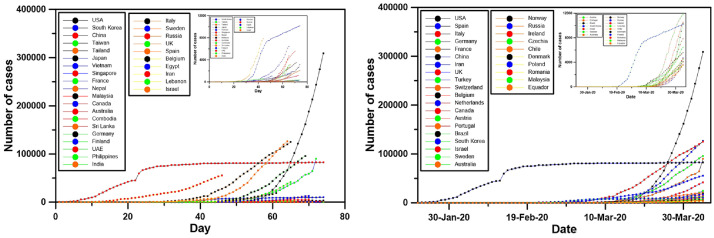
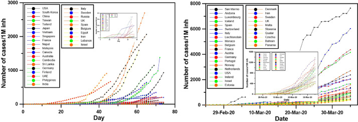
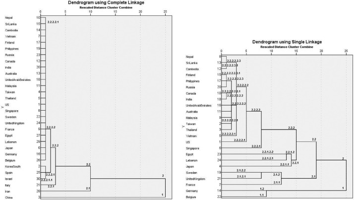
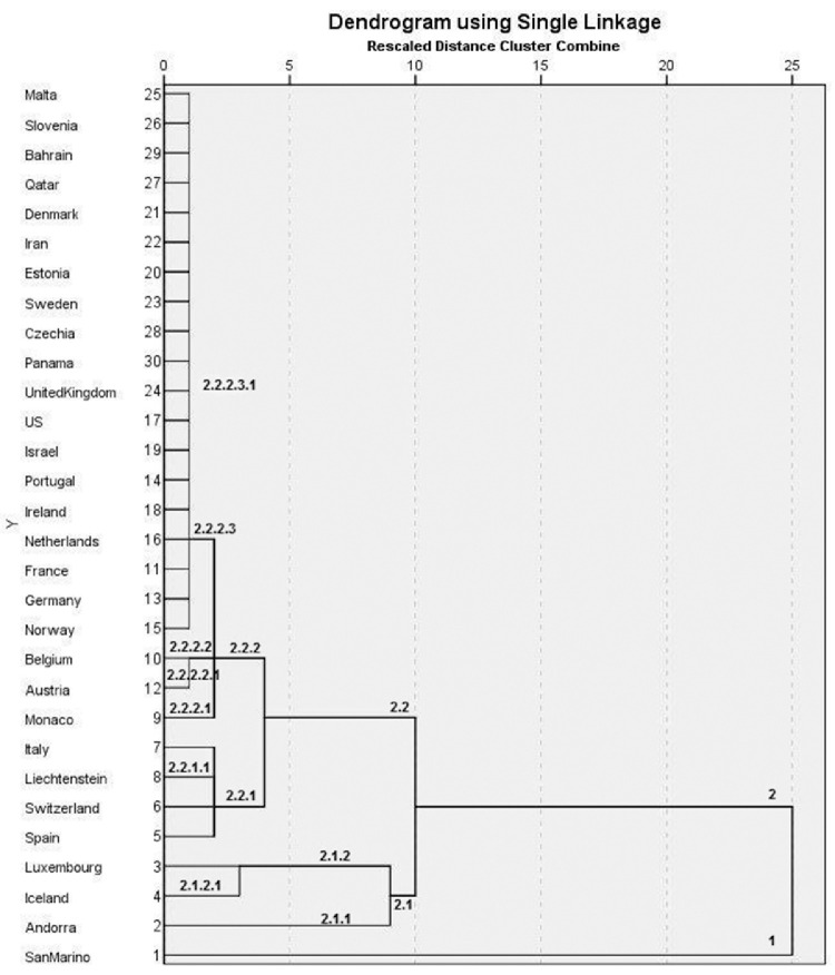
The initial data used here are extracted from the specific site created from John Hopkins University on COVID-19 (https://www.arcgis.com/apps/opsdashboard/index.html#/bda7594740fd40299423467b48e9ecf6). Due to low number of cases in the beginning of the pandemic in many countries, the first day used here is the 22th of January 2020, while the last day used is the 4th of April 2020. Excel 2019 was used to collect and integrate all the time series data. An algorithm to provide consistent clustering of various countries with respect to active cases, active cases per population and active cases per population and per area was developed. Mathematica 10 and SPSS 23 were used to run the relevant code. The final data are the number of cases per day and per date (Fig. 1), the number of cases/1 million inhabitants per day and per date (Fig. 3), the number of cases/population/land area per day and per date (Fig. 5). Moreover, this final dataset contains the results of our algorithm for the clustering of these countries for each one of the above cases (Figs. 2, 4, 6). The final dataset can be retrieved from Mendeley dataset, http://dx.doi.org/10.17632/kg72dst75p.1.

Fig. 1.

Evolution of cases from the first day for 30 countries with the older cases (left) and the 30 countries with the highest number of cases on April 4^th, 2020 (right). A zoom at the countries with the lowest values is shown.

Fig. 3.

Evolution of cases per 1 million inhabitants from the first day for 30 of countries with the older cases (left) and the 30 countries with the highest number of cases per 1 million inhabitants on April 4^th, 2020 (right). A zoom at the countries with the lowest values is shown.

Fig. 5.

Evolution of cases/population/land area from the first day for 30 of countries with the older cases (left) and the 30 countries with the highest number of cases/population/land area on April 4^th, 2020 (right). A zoom at the countries with the lowest values is shown.

Fig. 2.

Clustering of the countries using the cases per day data. Left: all countries with the data of the 45 first days. Right: clustering after the exclusion of the 6 bottom countries of the left figure.

Fig. 4.

Clustering of the countries using the cases/population per date data.

Fig. 6.

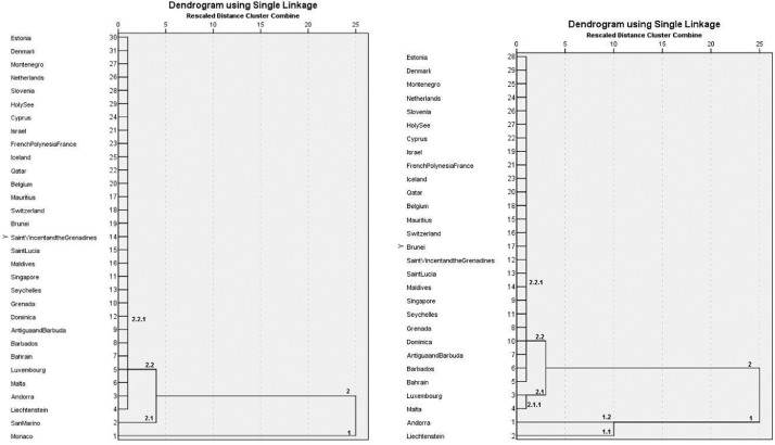
Clustering of the countries using the cases/population/land area per date data. Left: all countries. Right: clustering after the exclusion of Monaco and San Marino.

Fig. 1 shows, at the left, the evolution of cases in each country, starting from the first day of a COVID-19 case, for the thirty countries with the older cases (starting from 2th of January 2020) and, at the right, the 30 countries with the highest number of cases.

There is a significant difference in the evolution rate of COVID19 cases among the 30 countries of the left or of the right part of this figure. These countries follow some particular shapes:

• 1.The first shape corresponds to China: a very sharp increase the first days, an ever sharper after 21 days of the beginning (22th of January) and, then, a flattening of the curve after 15 more days.
• 2.The second shape corresponds to South Korea, where a similar curve as China appears, increase and flattening, but with very low number of cases comparing to China.
• 3.The third case corresponds to the countries where the cases appeared quite early, but they have a quite low number of cases until today (countries such as Vietnam, Thailand, Japan, Japan, Singapore or Nepal)
• 4.The fourth shape corresponds to the countries, such as USA, France, Germany, Italy, UK, Spain, Iran, Canada or Israel, where the cases appeared since several days, but the sharp increase appeared very recently with a very high number of cases during last days.

From this point of view, the countries can be clustered using our specific algorithm.

Using the hierarchical analysis, the clustering of Fig. 2 (left) is obtained using the par day data (left part of Fig. 1). As the countries have cases on a very different number of days, the clustering is based on the first 45 days of the time series. Fig. 2 shows that China, due to its particular shape, form one cluster alone. Next clustering isolates Iran from the other countries. The third clustering isolates Italy, the fourth a cluster of three countries: Israel, Spain and South Korea, while all other countries are together. A next calculation, not taking into consideration the previous countries, gives the results of the right part of Fig. 2. Here, Belgium and Germany form the first cluster. The second clustering isolates France UK and Sweden from the other countries. Inside this cluster, France is isolated form the other two countries. The clustering of the other counties gives two clusters, one of Japan, Lebanon and Egypt, with Japan being alone in a subsequent clustering. The cluster of the other countries isolates Singapore, then USA and then Vietnam, a cluster of all other countries, except Nepal, Sri Lanka and Cambodia being at the end.

The clustering using the date data is also performed. This figure completely changes the clustering. Here, USA is isolated from the first round, then China from the second, then Italy from the third. The fourth round groups 4 clusters, one of Spain, one of Germany, one of France and Iran and one of the other countries. Next clustering isolates UK, and then South Korea and UK from the other countries.

However, the previous analysis does not take into consideration the population of each country. A thousand active cases is China or in Luxembourg, countries with a population of almost 1.5 million people the first and 600,000 people the latter, don't have the same importance. For this reason, Fig. 3 shows the number of cases for each one million of inhabitants of each country.

Taking the population into consideration, the situation is completely different. San Marino is the country with the highest number of cases per population, followed by Andorra, Luxembourg, Iceland, Spain, Switzerland, Italy, Monaco, Belgium, France, Austria, Germany, Portugal, Norway, Netherlands and the USA, the country with the higher number of cases today. Left part of Fig. 2 shows that the thirty countries with the longest time series of cases are not always in the worst case. Again, the shapes of these countries are very different. As previously, four different shapes can be recognized, but the countries of the third and fourth group so not always remain in their respected groups.

Fig. 3 shows that the countries with the most critical situation are different than the countries revealed from Fig. 1.

Fig. 4 shows the clustering of these countries, in per date basis. San Marino is isolated from the first clustering. Second round isolated three countries: Andorra, Iceland and Luxembourg (Andorra is isolated from the other two in the next round) and the other countries. Next round isolates a cluster containing Spain, Switzerland, Liechtenstein and Italy, one of Monaco, Austria and Belgium (Monaco is isolated in the next round) and all the other counties remain together.

However, another parameter influencing the criticality of the situation is the surface area of each country. A thousand cases in Australia or Taiwan, two countries with quite similar population, but very different land area (Australia is 20 times larger than Taiwan) do not have the same effect on the COVID-19 epidemics. For this reason, Fig. 5 shows the results of Fig. 3 divided by the land area.

The situation is very different from Fig. 3. Fig. 5 reveals that the countries with the most critical situation are the small countries. Monaco is in the first case, far from the second country which is San Marino. Andorra, Lichtenstein, Luxembourg, Malta, Bahrein, Barbados, Antigua, Grenada and Singapore follow. Left part of Fig. 5 shows that the thirty countries with the longest time series of cases are is generally in less critical situation than the countries of the right side.

Hierarchical clustering of these countries (Fig. 6, left) shows that Monaco is isolated from the first round and San Marino from the second, while all other countries remain together. Removing Monaco and San Marino, a cluster with Liechtenstein and Andorra and one with Malta and Luxembourg is obtained, while all other countries remain together (Fig. 6, right).

Clustering with respect to active cases means that the elements of these clusters are countries that have similar time evolution of the active cases, which in turn means that they have faced similar stresses to the health system (with exception countries that performed extensive test to the general population; these countries are very few Taiwan, South Korea, Germany). Clustering with respect to active cases per population means that the countries that belong to the same cluster have experienced similar stresses to the society and the economy. Finally, clustering with respect to active cases per population per area is useful for driving conclusions about the impact of the disease that spreads more easily in densely populated areas (countries that have dense big cities are more vulnerable).

2. Experimental Design, Materials, and Methods

A requirement for “comparison of time series” is not a clear enough task since it includes many different aspects. Moreover, this topic is not a fully studied statistical problem to its entire mathematical completeness. The various challenges of the comparison between two or more time series include series with different sampling frequencies or different lengths or different scales. Furthermore, the question could focus on differentiating or likening certain characteristic values, means, trends, patterns of periodicity observed or forecast values. In the problem we want to analyze, in the present work, we need to find one meaningful way from the medical perspective to compare the time series of COVID-19 regarding active cases or similar variables.

The statistical analysis of different time series is a very useful method for many different disciplines. Some well-known methods are the Autoregressive Moving Average (ARMA) and Fourier analysis [1]. Regarding the utilization of different time series sometimes the goal is to uncover similarities and patterns that perhaps appear in the data. Various techniques have been used, such us indexing, classification, clustering or detection/identification of abnormal or specific characteristics [2], [3], [4], [5]. A similarity measure metric or non-metric is always used in such techniques. It is evaluated for two or more time series and returns a value for each one of them.

If someone will try to cluster countries with different COVID-19 time series using known algorithms and known statistical packages he will realize immediately that the clustering fails, and the results do not “look” correct. There are many reasons, different lengths, different orders of magnitude, many days with low numbers and sometimes suddenly sharp increases etc.

In the present paper, we have developed an algorithm that results to a consistent and reasonable clustering. The code was implemented partially in Mathematica and partially in SPSS. The criterion was the Euclidean distance between time series but with emphasis in the data of last days compared to initial days. Furthermore, we have also automatically adjusted a common length for all time series keeping the time length that contains large first derivatives and with and without disregarding the data after flattening of the curve (if such a behavior takes place). The overall algorithm follows the concept of hierarchical clustering [6,7].

A high-level description of the pseudo code follows. It was designed for time series x_j{t_i} with j=1...n, the number of time series of the variable x. Each country is denoted with the index j and i=1…m is the number of days.

• -Step 1: Keep or disregard terms of the time series in the flattening regime if such regime exists.
• -Step 2: Calculate all the rates of change for every pair x_j{t_i}, x_j{t_i+1}, and find number of day k_j when for the first time rate appears to be larger than 20% of the mean value of previous initial rates (that are always small in our time series).
• -Step 3: For all time series x_j{t_i} keep terms from i=k…m where k minimum of all k_j.
• -Step 4: Run the agglomerative clustering algorithm with single/complete linkage and Euclidean distance.

CRediT authorship contribution statement

Vasilios Zarikas: Conceptualization, Methodology, Software, Formal analysis, Writing - review & editing. Stavros G. Poulopoulos: Conceptualization, Methodology, Formal analysis, Writing - review & editing. Zoe Gareiou: Data curation. Efthimios Zervas: Conceptualization, Methodology, Software, Formal analysis, Writing - review & editing.

Declaration of Competing Interest

The authors declare that they have no known competing financial interests or personal relationships which have, or could be perceived to have, influenced the work reported in this article.

References

- 1.Shumway R.H., Stoffer D.S. Springer Verlag; New York: 2000. Time Series Analysis and Its Applications. [Google Scholar]
- 2.Warren Liao T. Clustering of time series data - A survey. Pattern Recognit. 2005;38:1857–1874. [Google Scholar]
- 3.Chin S.C., Ray A., Rajagopalan V. Symbolic time series analysis for anomaly detection: A comparative evaluation. Signal Processing. 2005;85:1859–1868. [Google Scholar]
- 4.Wei L., Keogh E. Semi-supervised time series classification. Proc. 12th ACM SIGKDD Int. Conf. Knowl. Discov. Data Min.; New York; 2006. pp. 748–753. [Google Scholar]
- 5.Alon J., Sclaroff S., Kollios G., Pavlovic V. Proc. IEEE Comput. Soc. Conf. Comput. Vis. Pattern Recognit. 2003. Discovering clusters in motion time-series data; pp. 1375–1381. [Google Scholar]
- 6.Ward J.H. Hierarchical Grouping to Optimize an Objective Function. J. Am. Stat. Assoc. 1963;58:236–244. [Google Scholar]
- 7.Sibson R. SLINK: An optimally efficient algorithm for the single-link cluster method. Comput. J. 1973;16:30–34. [Google Scholar]
Associated Data
This section collects any data citations, data availability statements, or supplementary materials included in this article.