Abstract
Weeds might be defined as destructive plants that grow and compete with agricultural crops in order to achieve water and nutrients. Uniform spray of herbicides is nowadays a common cause in crops poisoning, environment pollution and high cost of herbicide consumption. Site-specific spraying is a possible solution for the problems that occur with uniform spray in fields. For this reason, a machine vision prototype is proposed in this study based on video processing and meta-heuristic classifiers for online identification and classification of Marfona potato plant (Solanum tuberosum) and 4299 samples from five weed plant varieties: Malva neglecta (mallow), Portulaca oleracea (purslane), Chenopodium album L (lamb's quarters), Secale cereale L (rye) and Xanthium strumarium (coklebur). In order to properly train the machine vision system, various videos taken from two Marfona potato fields within a surface of six hectares are used. After extraction of texture features based on the gray level co-occurrence matrix (GLCM), color features, spectral descriptors of texture, moment invariants and shape features, six effective discriminant features were selected: the standard deviation of saturation (S) component in HSV color space, difference of first and seventh moment invariants, mean value of hue component (H) in HSI color space, area to length ratio, average blue-difference chrominance (Cb) component in YCbCr color space and standard deviation of in-phase (I) component in YIQ color space. Classification results show a high accuracy of 98% correct classification rate (CCR) over the test set, being able to properly identify potato plant from previously mentioned five different weed varieties. Finally, the machine vision prototype was tested in field under real conditions and was able to properly detect, segment and classify weed from potato plant at a speed of up to 0.15 m/s.
Keywords: Agriculture, Computational intelligence, Computer simulation, Video processing, Computer engineering, Food science, Food engineering, Agricultural engineering, Agricultural soil science, Agricultural technology, Horticulture, Video processing., Plant competition, Meta-heuristic algorithms, Classification, Site-specific spraying, Machine vision
Agriculture; Computational intelligence; Computer simulation; Video processing; Computer engineering; Food science; Food engineering; Agricultural engineering; Agricultural soil science; Agricultural technology; Horticulture; Video processing.; Plant competition; Meta-heuristic algorithms; Classification; Site-specific spraying; Machine vision.
1. Introduction
Weeds are among one of the biggest challenges in agriculture given their direct competition with crops in consuming resources such as soil nutrients and water. Weeds tend to follow a pseudo random distribution in various patches of land in agricultural fields. Proportional to the type, volume and distribution of weed in field and also the characteristics of soil –like soil humidity, nutrients in soil, and soil pH– so is the level of agricultural crop product performance influenced (Papamichail et al., 2002). An effective and applicable management that is consistent to the correct period of fighting against weeds must be used in order to succeed. Zimdahl (1993) believes that the best period for fighting against weeds is the period starting after cultivating seeds and lasting until the competition of weeds affect the performance of agricultural crop yield. This period is different regarding the type of weed and cultivated product.
Therefore, these conditions must be carefully investigated before determining the method and calendar in fighting weeds. Manual method is the most elementary method for fighting weeds. In this method, the removal of weed from field is performed using a human-operated tool. This method is not applicable for current wide lands because of high cost, being boring and needing high human force. Mechanical methods (using tractor and agricultural implements) are applicable for fighting with weeds for row crops, such as corn, sugar beets, wheat and potatoes. About a 50% of weeds between two rows of crop can be controlled using this methodology.
Eyre et al. (2011) believe that the use of mechanical methods has negative effects on agricultural products and environment, since they destroy agricultural crops and generate soil erosion. Use of chemical methods became common concurrent with herbicides discovery during the end of 1940s and this method is still popular among farmers (Gianessi and Reigner, 2007).
According the study of Gianessi and Reigner (2007), the use of herbicides in the state of Mississippi had a $10M saving as compared to manual control of weeds. Despite herbicides were successful in controlling weeds, they had destructive effects on environment, human health, animals and plants. For this reason, different researchers are nowadays following several methods that may minimize these destructive effects of general herbicide application. Site-specific spraying can be considered as one of the most important methods that is being investigated by different researchers these days. In this method, herbicide spray is minimized and only applied where necessary, only to weeds. In order to make this method operational, machine vision is often a proper choice among researchers in the field.
Machine vision has numerous applications that have been previously mentioned by several authors, such as (Banerjee et al., 2018; Mukherjee et al., 2017a, 2017b; Sudeep et al., 2018; Bhattacharyya et al., 2018), to cite a few. In addition, neural networks play a main role in machine vision field. Application of Neural Networks has been previously mentioned by various authors, such as (Jayasinghe et al., 2019; Kim et al., 2019; Dash et al., 2018), to cite a few.
Generally speaking, machine vision systems are often formed by two main parts. First part is responsible for identifying plants and extracting features from them while second part is responsible for their classification (Hamuda et al., 2016). In this regard, a number of researchers have identified weeds by using spectral reflectance, see Pantazi et al. (2016) for instance. They implemented a method based on machine vision by emphasizing that weeds have a destructive effect on yield of agricultural products and were able to identify maize plant and the following ten weed types: Ranunculus repens, Cirsiumarvense, Sinapisarvensis, Stellariamedia, Tarraxacumofficinale, Poaannua, Poligonumpersicaria, Urticadioica, Oxaliseuropaea and Medicagolupulina. In their suggested method, weeds and corn are separated using the difference in spectral reflection. Spectral features were extracted using an imaging system of high-spectral response mounted on a platform. The speed of platform movement was 0.09 m/s, 164 samples were used from maize plant and also for each weed type (110 train and 54 test samples) for classification purposes. They used four mixtures of Gaussians classifiers, self-organizing feature maps (SOFM), support vector machine (SVM) and auto-encoder network as classifiers. Results showed that the methods of mixture of Gaussians and SOFM identified maize crops with 100% accuracy; while the methods of SVM and auto-encoder network did with accuracies of only 29.63% and 59.26%, respectively. Correct classification percentage for different species of weed was in the range 31%–98% (mixture of Gaussians), 53%–94% (SOFM), 12.98%–68.52% (SVM) and 9.63%–68.52% (auto-encoder network). In summary, suggested method has maximum accuracy above 90% only in identifying 4 weed types; thus, in the event of being used in field, system error is rather high in identifying the remainder weed types.
The use of color features and their combinations was intended in order to separate weed and crop in (Kazmi et al., 2015). They identified sugar beet and thistle weed using vegetation indices. They used an ordinary visible-range camera under natural light conditions and took 474 photos of sugar beets and thistle weed. These images were divided based on the level of illumination, age and scale, into six different groups. First and second groups include seventh week cultivated sugar beet date, location of camera 45 cm above ground level and under both sunlight and shadow conditions. Third and fourth groups comprise tenth week sugar beet in shadow with camera at distances of 60 and 70 cm above ground level; finally, fifth and sixth groups include twelfth week sugar beet, position of camera at 70 cm above ground level and under two illumination conditions of direct sunlight and shadow. A total of 14 color indicators were extracted from each image. Among these 14 extracted features, 3 selected features were used for classification purposes, comprising excess green, green minus blue and color index for vegetation extraction features. Two methods of linear discriminant analysis and Mahalanobis distance were used to classify both types of plants. Results showed that the classifier system performed with an accuracy of 97.83%, in the best case. This accuracy is acceptable, but using color indices solely for identifying several kinds of weed in open-air field may not be sufficient.
Using machine vision for fighting weeds between rows in row crops is under attention of many researchers. Generally speaking, fighting weeds between rows in row crops includes two main stages. First stage is the identification of crop row and the second is the identification of plants between each two adjacent rows. In this regard, Tang et al. (2016), after investigating uniform herbicide spraying on all field surface, concluded that this spray method causes the pollution of environment and decreases the quality in agricultural crops, in addition to wasting herbicide and working forces; therefore, they suggested the automatic identification of weeds and selective spraying for sustainable development of agriculture. Their research was implemented concerning site-specific spray under different light conditions in maize farms. In this research, 1300 photos were taken under different light conditions (sunny and cloudy). Camera was installed on tractor console. For identifying central line of crop row, the combination of two methods (vertical projection and linear scanning methods) was used. The classic weeds infestation rate (WIR) method was used for real-time identification of crop rows via minimizing the rate of Bayesian error. Results showed that the suggested method has superiority as compared to Bayesian and SVM. Results are not applicable for identifying different weed types from each other, because only crop row is identified and all plants between rows are identified as weeds, regardless of their type.
Guerrero et al. (2012) performed a study on separation of green-color plants from background. They believe that, automatic separation of weed and crop in precision agriculture is a very important issue, being investigated by different researchers these days. Nowadays, optical imaging sensors have an increasingly important role; authors suggested a new method based on SVM for identifying plants using masked and un-masked green color spectral component. Learning phase of suggested method includes three main stages:
-
1.
Identification of greenness using the value of threshold determined via Otsu's method for obtaining binary image (two classes were determined).
-
2.
Identification of support vector used for each class using SVM.
-
3.
Calculation of mean value for all sets of support vector that causes the creation of a valid threshold for separating masked and unmasked plants.
Results showed that the performance of the suggested system is acceptable and has no problem to be used in machine vision systems. However, this method has only the capability of separating green plants from background and needs to be further extended for proper use in specific location operations.
Herbicide application is among most important issues that can directly affect human health. Herbicides have long been used as one of the main methods to eliminate weeds. With the development of mechanization, herbicides were applied uniformly in all parts of farms land. Two major drawbacks of uniform spraying are as follows: first, there may be some parts of land which lack of weeds, however, they are also sprayed unnecessary due to uniform field spraying. Second, there is no possibility of weed-type dependent spraying and this ultimately increases the final costs of agriculture yield production. In order to overcome the shortcomings mentioned, the use of precision agriculture is recommended. Precision agriculture has different roles including optimal site-specific spraying of different herbicides in cultivable lands. Therefore, the alternative method used in precision agriculture is consistent spraying with the type, location and number of weeds. As a consequence, the type, location and number of weeds need to be identified before spraying.
The aim of this study is to present an automatic machine vision prototype in the visible range based on video processing and network-cultural classification algorithm for accurate identification and classification of Marfona potato plant and five weed species, as listed next: Malva neglecta (mallow), Portulaca oleracea (purslane), Chenopodium album L (lamb's quarters), Secale cereale L (rye) and Xanthium strumarium (coklebur), which could exist in stack and inside crop row in potato field, in order to detect, segment and classify them for potential site-specific herbicide spraying application, among other possible purposes.
2. Materials and methods
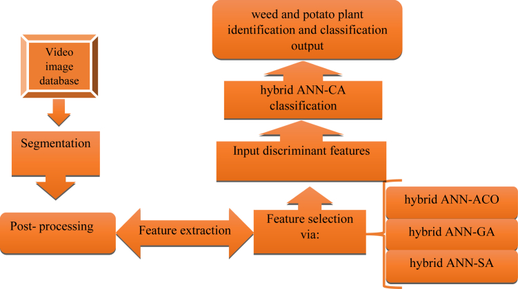
The proposed weed detection, segmentation and classification system prototype has two main sub-systems, comprising video processing and classification. Figure 1 shows the flowchart of proposed visible-range automatic video identification and classification of weed species in potato field prototype.
Figure 1.
System prototype flowchart for the visible-range automatic video detection and classification of five invasive (weed) species in potato field. Acronyms: ANN Artificial Neural Network, CA: Cultural Algorithm, AC: Ant Colony, GA: Genetic Algorithm, SA: Simulated Annealing.
2.1. Farm settings and data collection
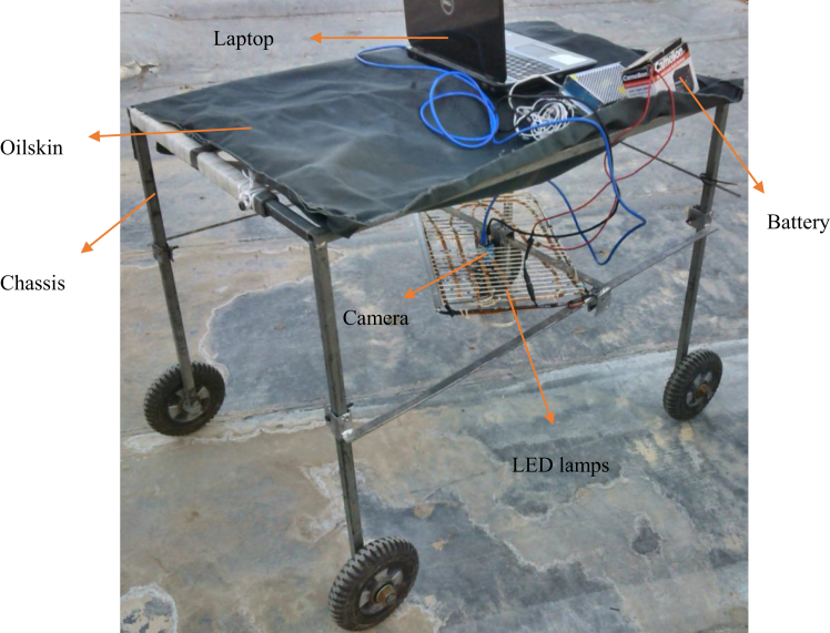
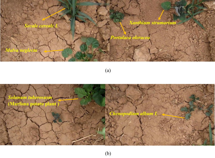
First stage in designing the proposed machine vision system prototype for potentially spraying different herbicides on different weed is data collection. For this reason, first a specific purpose chamber was designed (Figure 2) in order to properly record video data. This chamber is constituted of two main parts: lighting and video camera. Camera used was model DFK 23GM021, 1/3 inch Aptina CMOS sensor (MT9M021), 1280×960 (1.2 MP), up to 115 fps, ImagingSource, GigE color industrial camera, Germany. Lighting condition was set up by white color LED lamps with an intensity of 327 lux. During filming, the camera was attached to body tightly at a fixed height of 45 cm from ground level. An oilskin enclosed all chamber to avoid environmental lights from entering the chamber. Two agricultural fields of Marfona potato variety were selected for filming (total area of 6 ha) in Kermanshah province, Iran (longitude: 7.03°E; latitude: 4.22ºN). It is worth noting that filming was performed in the sixth week after potato seedtime. Filming speed was set at 0.15 m/s, approximate. Fields had 5 different weed types (Figure 3). Table 1 shows common English and scientific names as well as number of different weed plants used in this work, totaling 4299 different plants among the five weed species.
Figure 2.
Specific hand-build chamber for potato field filming purposes.
Figure 3.
Four video frame examples of potato plant and five different invasive species recorded in potato field with DFK 23GM021, 1/3 inch Aptina CMOS sensor, 1280×960, ImagingSource, GigE (Germany) color industrial camera: (a) left: Malva neglecta and Secale cereale L, (a) right: Portulaca oleracea and Xanthium strumarium, (b) left: Solanum tuberosum (Marfona potato plant) (b) right: Chenopodium album L.
Table 1.
English and scientific name of five different potato field invasive (weed) plant species and the number of weed plants in each class (totaling 4299 invasive plants).
| English name | Plant specie |
||||
|---|---|---|---|---|---|
| rye | lamb's quarters | purslane | mallow | cocklebur | |
| Scientific name | Secale cereale L | Chenopodium album L | Portulaca oleracea | Malva neglecta | Xanthium strumarium |
| Number | 654 | 509 | 202 | 1502 | 1432 |
2.2. Segmentation and post-processing
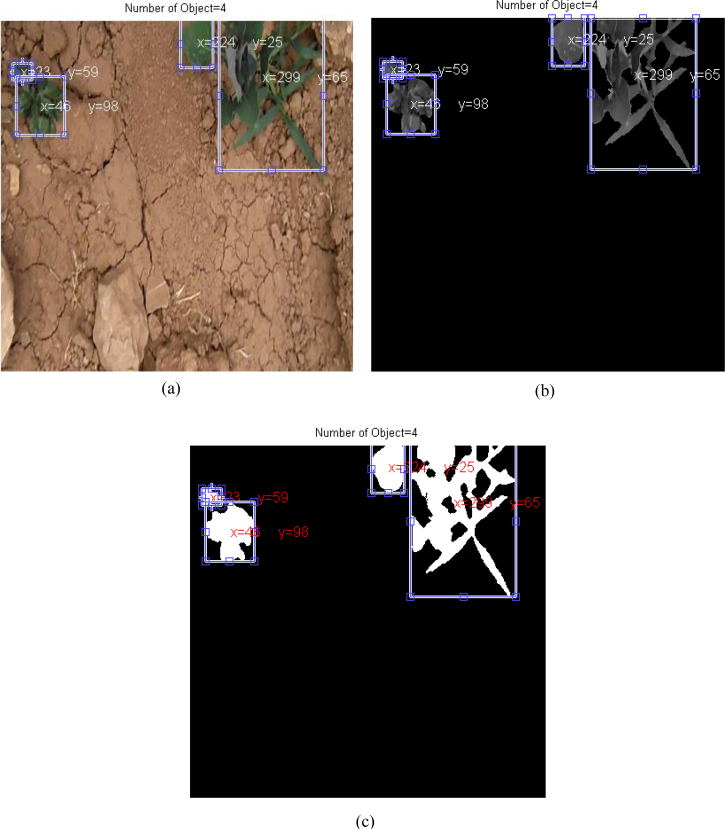
Videos recorded in farms need to be analyzed at frame level. Indeed, various image processing operations must be applied on them. The first step is image segmentation. Generally speaking, segmentation comprises two stages. First segmentation stage is plant separation from background and second segmentation stage is object identification (object defined as continuous pixels in a frame) in each frame. Regarding background removal, a proper separation threshold was applied. In this study, after investigating different frames and applying different thresholds, we concluded that best fixed threshold can be defined in Eq. (1):
| (1) |
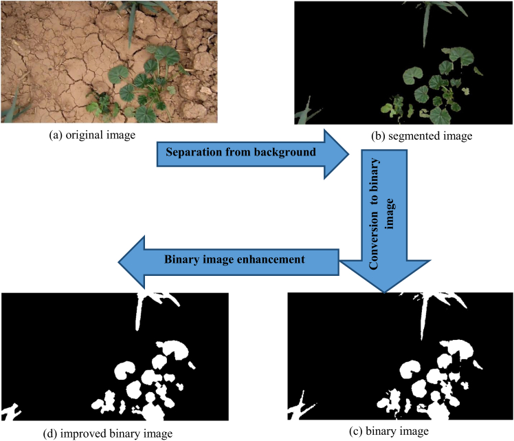
Eq. (1) states that the pixels with green component larger or equal to red or blue components, will remain in image (foreground) and otherwise pixels will be considered as background and thus removed from image. Regarding object identification, all available objects in a frame are identified and kept in order to perform other subsequent image processing operations. Figure 4 shows an object identification segmentation example. As it can be observed in this figure, four objects are identified. Each object must be converted to binary image in order to properly extract shape features; during segmentation state, some noise is still visible on image that must be removed using post-processing operations. In this study, the noise removal was performed using a closing operation and a binary image was generated with high accuracy. Figure 5 shows an example of different image segmentation stages. Finally, a total of 4784 video frame objects were recognized after segmentation operation.
Figure 4.
An example of object identification: (a): original image {original.fig}, (b): grayscale image {gray.fig} and (c): binary segmented image {binay.fig}. Frame image objects Cartesian coordinates are also displayed. The origin of coordinates in set in the upper left corner of image. Note: Corresponding interactive Matlab .fig figure file names, are indicated between brackets.
Figure 5.
Image segmentation example: (a): original image {original image.fig}, (b): segmented image {segment image.fig}, (c): binary image {binary image.fig}, and (d): improved binary image {improvement image.fig}. Note: Corresponding interactive Matlab .fig figure file names, are indicated between brackets.
2.3. Feature extraction
In order to identify objects extracted from video frames, there is the need to use features extracted from objects. For this purpose, object features were conveniently extracted from five different feature types: texture features based on the gray level co-occurrence matrix (GLCM), color features, spectral descriptors of texture, moment invariants and shape features.
2.3.1. Texture features based on GLCM
GLCM texture features are extracted based on loci of pixels with equal value. For example, consider the matrix shown in Figure 6(a); this matrix has four gray levels (1, 2, 3, 4). Figure 6(b) shows horizontal co-occurrence matrix corresponding to Figure 6(a) matrix. Co-occurrence matrix is a 4×4 size matrix, since there are four different gray levels. In Figure 6(b) matrix, the element (1,1) is equal to 1, because there is only one state in Figure 6(a) in which a pixel with the value 1 is in the right side of another pixel with value 1. Several features are extractable based on this matrix. In this study, eight features including, difference variance, correlation, sum of squares, sum of variances, inverse difference normalized momentum, cluster prominence, standard deviation and the coefficient of variation, are extracted, as shown next.
Figure 6.
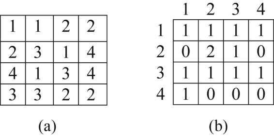
An example of the method for co-occurrence matrix creation in the GLCM texture features framework: (a): original matrix, (b): co-ocurrence matrix.
After calculating co-occurrence matrix , normalization step takes place using Eq. (2) (Marques, 2011), and further used for feature computation as shown next:
| (2) |
where is co-occurrence matrix and being L the total number of gray levels.
-
‒
Difference variance (DVAR): difference variance is a measure of local variability that is calculated using Eq. (3):
| (3) |
where DENT is the so-called Difference Entropy defined next:
| (4) |
in Eq. (4) is in turn calculated using Eq. (5), from normalized co-ocurrence matrix:
| (5) |
-
‒
Variance: Variance shows distribution of the degree of dispersion of gray levels in co-occurrence gray level matrix. If gray levels of image are severely extended, sum of squares is big (Abouelatta, 2013). Variance is calculated using Eq. (6).
| (6) |
being the mean value.
-
‒
Standard deviation: is defined as the square roof of variance:
| (7) |
-
‒
Correlation: is a degree of linear dependency in gray levels on neighbor pixels and/or specific points. Correlation with a value near to one shows linear relation between gray levels of pixel pairs. Correlation is calculated as shown next using Eq. (8):
| (8) |
where and are mean and and are standard deviation values of rows and columns, respectively, in normalized co-ocurrence matrix .
Co-ocurrence matrix mean is defined next in Eq. (9):
| (9) |
-
‒
Sum of variance: sum of variance is total difference to mean value and is defined as shown in Eq. (10) (Shidnal, 2014):
| (10) |
where SENT is Sum Entropy defined next:
| (11) |
being in turn defined next:
| (12) |
-
‒
Inverse difference normalized momentum (IDN): if the pixels of gray level co-occurrence matrix are similar to each other, IDN has a high value. Therefore, when the image is locally homogeneous, this value will be big (Abouelatta, 2013). IDN is computed by using Eq. (13) shown next:
| (13) |
-
‒
Cluster prominence: this is a measure of the degree of asymmetry in image; when value of cluster prominence is high; image has lowest asymmetry and vice versa. Cluster prominence is defined next in Eq. (14) (Yang et al., 2012):
| (14) |
-
‒
Variability coefficient: this is defined as the ratio of the standard deviation to co-occurrence matrix mean, see Eq. (9).
2.3.2. Texture spectral descriptors
Spectral measurement of texture is based on Fourier spectrum. This spectrum describes alternative patterns and/or almost any 2-dimensional alternation in an image. Fourier spectrum is better described in the polar coordinate system (based on radius and angle ), because anticipation of spectral features with spectral description in polar coordinates as function is simple. In previous function, is spectral function and and are variables of polar coordinate system; therefore, function can be considered as two one-dimensional functions and for each direction and each frequency , respectively. shows a spectrum behavior along radius for constant values of , while shows spectral content along a circle centered at the origin of coordinates for constant values . Eqs. (15) and (16) result in overall texture description based on the following two functions:
| (15) |
| (16) |
where is the radius of a circle with center at the origin; this way, three features including mean, standard deviation and variance, were calculated for and in this study.
2.3.3. Color features
One of the most important feature types for segmentation and also classification of different plants is color features. Color features in different color spaces give different results. It is well-known that if filming is performed using RGB color space, other color spaces like HSV, HIS, CMY, YCbCr and YIQ can be directly obtained using different matrix convert equations from RGB color space color coordinates. In this study, a total of 13 features were extracted from different color spaces. Extracted color features follow next: standard deviation of hue component (H) in HSV color space, mean value of hue component (H) in HSI color space, mean yellow component (Y) in CMY color space, standard deviation of yellow component (Y) in CMY color space, mean of all three components in CMY color space, computed as , standard deviation of saturation component (S) in HSV color space, mean value of hue component (H) in HIS color space, mean blue-difference chrominance Cb component in YCbCr color space, standard deviation of in-phase component (I) in YIQ color space, mean green component (G) in RGB color space, standard deviation of green component (G) in RGB color space, standard deviation of blue component (B) in RGB color space, and standard deviation of red component (R) in RGB color space.
2.3.4. Moment invariants
Direction of growth for plant leaves in agricultural fields is variable; for example, a leaf can be oriented towards east and another one towards west on the same stem of plant. At the same time, the size of plants is also different, some of them are big, some average and some small. Given camera movement in farm for site-specific management of weeds, the above mentioned limitations are hard to solve since recording camera in farm is moving; therefore, it seems reasonable that features that are independent of size and direction may have application in classification. For this reason, in this study we used five moment invariants features: first, second, sixth, seventh moment invariants and also the difference of first and seventh moment invariants (Gonzalez et al., 2004). Eqs. (17), (18), (19), (20), (21), (22), (23), (24), and (25) calculate these features, as shown next:
| (17) |
| (18) |
| (19) |
| (20) |
where is defined as in next Eq. (21):
| (21) |
where
| (22) |
Value of is calculated as shown next:
| (23) |
where
| (24) |
Finally, in Eq. (24) is defined as follows:
| (25) |
2.3.5. Shape features
Because of the difference in shape of leaves in different weed plants, using shape features may be beneficiary for their classification. For this reason, 8 shape features were extracted: length, width, area, perimeter, logarithm of length to width ratio, ratio of shape perimeter to outer rectangle perimeter including object shape inside, width to length ratio, and ratio of area to length, in accordance to the following definitions (Gonzalez et al., 2004):
-
‒
Length: main oval axis that has second equal momentum with the intended area (pixels).
-
‒
Width: minor oval axis that has second equal momentum with the intended area (pixels).
-
‒
Area: number of existing pixels inside an image region.
-
‒
Perimeter: perimeter of an area is calculated counting the number of pixels on its boundary.
2.4. Feature selection
Important criteria in online operations is processing time; therefore, computation time must be minimized as much as possible. Site-specific spray is one of online operations; using all extracted features increases processing time and also may create mistake for classification system due to poor generalization capability. For this reason, selection of features is an appropriate way to solve this problem. Different meta-heuristic methods exist for feature selection. In this paper, three methods were used: hybrid artificial neural network - ant colony (ANN-ACO), hybrid artificial neural network - simulated annealing (ANN-SA) and hybrid artificial neural network - genetic algorithm (ANN-GA), as will be described soon after.
The procedure has two parts: first all extracted (computed) features are considered as a vector, and in the next step, smaller vectors of features, for example, vectors with feature numbers 8, 6, 10, and others are selected as being highly discriminant by means of various suboptimal feature selection methods, including GA, ACO and SA, and then those selected features are sent as input to the multilayer perceptron neural network for classification purposes. In fact, the input of the neural network are the selected feature vectors from the GA, ACO and SA methods, and network output are the classification of the six different plants considered (five weed plants and Marfona potato plant). Input samples to the network are split by a ratio of 70% training, 15% validation and remaining 15% testing (disjoint) sets. The mean square error of each input vector into the multilayer perceptron neural network is recorded and finally the vector having the least mean square error, is chosen as the optimal vector and features within that vector are selected as effective discriminant features, discarding all other features.
2.4.1. Ant colony (ACO)
Ant colony (ACO) is an optimization technique used for solving optimization problems. It is based on ant movement in finding nutrients. Ants travel a path in order to find food and they leave a material known as pheromone proportional to the length of path and quality of nutrients. Other ants smell pheromone and travel the same path and therefore the value of pheromone is amplified; this way, the paths that have shorter length from nest to food source have higher amount of pheromone and are selected as optimal paths (Lin et al., 2016).
2.4.2. Genetic algorithm (GA)
Genetic algorithm (GA) is one of the most powerful optimization methods inspired by nature behavior. Indeed, this algorithm is established based on natural complement principles. As a general law, only those strongest animals win in the fight on food and life and therefore have the possibility of breeding. This superiority comes from individual features and their genes. By breeding, these genes are replicated and better children are generated. Therefore, by consecutive implementation of selection of species, best population and breeding via them, new populations with higher consistency and survival probability are created resulting in better and more resources available by the members of society (Garg, 2016).
2.4.3. Simulated annealing (SA)
Simulated annealing (SA) is based on annealing operation over metals. Annealing operation is performed for achieving the most stable and lowest energy state among available stable states for material. First, the material is melted and then the temperature is slowly decreased step by step (in each stage of temperature decrease, operation of temperature decrease is stopped whenever material temperature reaches a low energy equilibrium state) and this is continued until the material becomes solid. If the level of temperature decrease is performed in a convenient manner, annealing performance reaches to its optimal goal. On the contrary, if the material is rapidly cooled, the body reaches a near to but sub-optimal state that has not minimum energy (Zameer et al., 2014).
2.5. Classification
An important last stage in machine vision systems is classification stage. Indeed, discriminant features selected in previous stage are sent to classification unit as input in order to identify different plants based on those input features. If an appropriate classifier is not used, the machine vision system will behave poorly. Different classifiers exist in statistical areas and artificial intelligence for classification. Results showed that if the amount of data is high, number of inputs in classifier is high and/or the number of classes is high, then most artificial intelligence methods behave better than statistical methods. In the current study, the hybrid artificial neural network -cultural algorithm (ANN-CA) classifier is used for classification purposes. Cultural algorithm performs optimization actions similar to genetic algorithm. Whereas in genetic algorithm, natural and biologic evolution is intended, in cultural algorithm, cultural evolution and influence of cultural and social space is considered and optimized. In a society, the person who is more under attention and is more recognized has more influence on cultural evolution. For instance, influencing people may influence on the way of talking, walking and dressing up, to name a few. Final aim of CA is finding these elites and their development for cultural complement (Ali et al., 2016).
The multilayer perceptron neural network has five adjustable parameters in MatLab, which determine the accuracy of the network based on its optimal setting, including: the number of neurons, the number of layers, the transfer function, Backpropagation network training function, and Backpropagation weight/bias learning function. In this study, the number of neurons in each layer could be at least 0 and maximum 25; the number of layers at least 1 and maximum 3; the transfer function for each layer was selected from the following transfer functions list (MatLab): logsig, purelin, hardlim, compet, hardlims, netinv, poslin, radbas, satlin, satlins, softmax, and tribas; Backpropagation network training function was selected from: trainlm, trainbfg, trainrp, traingd, traincgf, traincgp, traincgb, trainscg, train, traingda, traingdx, trainb, trainbfgc, trainbr, trainbuwb, trainc, traingdm, trainr, and trains (MatLab). Finally, Backpropagation weight/bias learning function was chosen from: learngdm, learngd, learncon, learnh, learnhd, learnis, learnk, learnlv1, learnlv2, learnos, learnp, learnpn, learnsom, learnsomb, and learnwh (MatLab). The objective of using a CA algorithm is to send different vectors among these parameters to suboptimal adjust the parameters of the multilayer perceptron neural network. For example, consider vector v = [5,6,12, tansig, poslin, tribas, trainlm, learnk]. Previous vector selection implies that the structure of the determined optimal neural network by the CA algorithm would have: three hidden layers with number of neurons 5, 6, and 12, respectively, and transfer functions are tansig, poslin, and tribas, respectively. It also shows that Backpropagation network training function and Backpropagation weight/bias learning function are trainlm and learnk, respectively. After each vector is sent as input to the CA algorithm, the mean of the mean square error of each tested vector will be recorded, and finally the vector that has least average of squared error is chosen as an optimal vector, being its members selected as optimal values of the adjustable network parameters. Finally, at each stage in which the selected feature input vector is sent to the multilayer perceptron neural network classifier, the total input data samples are divided into three disjoint training (70%), validating (15%), and testing (15%) sets.
3. Results and discussion
3.1. Selection of discriminant features
Selection of effective discriminant features is one of the most important stages in machine vision system design. The lower the number of features is, the higher the speed of machine vision system is. As mentioned before, three methods are used in this study for selecting effective features: hybrid ANN-ACO, hybrid ANN-SA and hybrid ANN-GA. Table 2 shows selected features using three previously mentioned methods.
Table 2.
Six color video frame image discriminant features selected by three hybrid meta-heuristic methods: ANN-ACO, ANN-SA and ANN-GA.
| Method | Selected discriminant features |
|---|---|
| hybrid ANN-ACO | length to width ratio, variance difference, standard deviation H in HSV color space, correlation, mean Y component in CMY color space, sum of squares |
| hybrid ANN-SA | mean CMY components, standard deviation S in HSV color space, sum of variance, inverse difference normalized momentum, cluster prominence, variance difference |
| hybrid ANN-GA | standard deviation of S component in HSV color space, standard deviation of S component in HIS color space, mean Cb component in YCbCr color space, standard deviation of I component in YIQ color space |
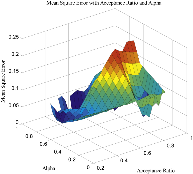
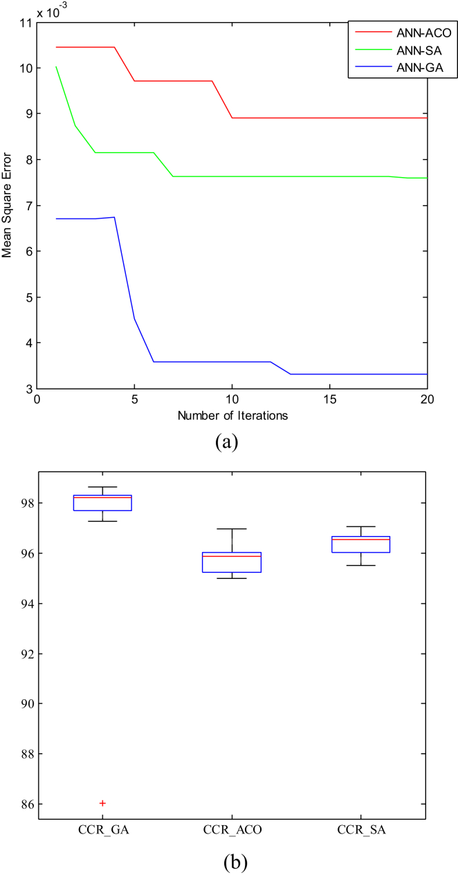
Now, in order to find most effective features among these three groups, each group of features was sent for classification as input to hybrid ANN-CA. Meta-heuristic algorithms including cultural algorithm have different parameters which are often determined using try and error, and therefore it is possible that these parameters are not optimal. For this reason, particle swarm algorithm was used in this study for finding optimal values of the two parameters in cultural algorithm, i.e. alpha coefficient (a coefficient similar to mutation in genetic algorithm) and acceptance ratio (number of individuals influenced on population). Figure 7 shows three-dimensional graph for mean square error (MSE) over these two parameters. In fact, for each adjustment on these two parameters, hybrid ANN-CA classifier performed classification and the MSE was computed. Results showed that optimal value for alpha coefficient and acceptance ratio are equal to 0.692 and 0.834, respectively. After optimizing these two parameters, selective features were entered by each method as input for classification purposes with the help of a hybrid ANN-CA. Figure 8 shows results on feature selection in classification capability for the following three hybrid methods: ANN-GA, ANN-ACO, and ANN-SA. Figure 8(a) shows results about MSE during 20 repetitions. As it can be observed, selected features by the hybrid ANN-GA method clearly outperforms other two methods. Figure 8(b) shows boxplots of classification accuracy (correct classification rate CCR, in %), over 20 repetitions. Again, clearly hybrid ANN-GA is ahead of its partners. This way, selective (discriminant) features can be used as effective selected features by genetic algorithm and classifier model can be potentially used for online operations on video detection and identification of weed species, and on in-field site-specific spraying of herbicide, amongst others. At the same time, Table 3 shows the optimal structure and size of neural networks for each model: hybrid ANN-ACO, ANN-SA and ANN-GA, comprising training and transfer functions.
Figure 7.
Three-dimensional graph of the mean square error (MSE) with varying alpha and acceptance rate hybrid ANN-CA parameters {Alpha_Acceptance Ratio.fig}. Note: Corresponding interactive Matlab .fig figure file names, are indicated between brackets.
Figure 8.
Performance comparison of ANN-GA, ANN-ACO, ANN-SA over 20 iterations (test set). (a): mean square error (MSE) for each iteration {Compaire.fig} (b): boxplots on classification accuracy, Correct classification rate (CCR) in % {CCR.fig}. Note: Corresponding interactive Matlab .fig figure file names, are indicated between brackets.
Table 3.
Optimized classifier parameters in three different hybrid supervised learning architectures: ANN-ACO, ANN-SA, and ANN-GA.
| Hybrid ANN architecture | Number of neurons | Number of layers | Transfer function | Backpropagation network training function | Backpropagation weight/bias learning function |
|---|---|---|---|---|---|
| ANN-ACO | first layer: 15, second layer: 15, third layer: 15 | 3 | first layer: tansig, second layer: tansig, third layer: tansig | trainlm | learngdm |
| ANN-SA | first layer: 15, second layer: 15, third layer: 15 | 3 | first layer: tribas, second layer: tribas, third layer: tribas | trainlm | learngdm |
| ANN-GA | first layer: 15, second layer: 12, third layer: 15 | 3 | first layer: tansig, second layer: tansig, third layer: tansig | trainlm | learnwh |
3.2. Classification
3.2.1. Classification using hybrid artificial neural network - cultural algorithm (ANN-CA) classifier
Last stage in the design of the here proposed machine vision system is classification. In this study, hybrid ANN-CA is used for classification purposes. All 4784 objects extracted from farm video are divided into two groups of training and validation (80% of data, i.e. 3825 objects) and test (20% of data, i.e. 959 objects). Table 4 shows classification results of potato plant and five different types of weed that are classified by this method, over the test set. In this table, class numbers 1 to 6 show 1-Malva neglecta (mallow), 2-Portulaca oleracea (purslane), 3-Chenopodium album L (lamb's quarters), 4-Secale cereale L (rye), 5-Marfona potato plant (Solanum tuberosum) and 6-Xanthium strumarium (cocklebur), respectively. As it can be observed, classification results are displayed as a 6×6 confusion matrix, given that we have six different classes in problem at hand. Confusion matrix compares true versus estimated classification output. Table 4 shows that 16 object samples are misclassified from a total 959 test set object samples. Highest level of wrong classification is found in Chenopodium album L class. Among 120 samples of Chenopodium album L weeds, 5 samples are misclassified with 4.17% classification error. Lowest level of wrong classification is found in Solanum tuberosum (Marfona potato plant) class, where all object samples are correctly classified. Results showed that Xanthium strumarium and Chenopodium album L weeds have high similarity under selected features (3 samples of Xanthium strumarium are misclassified in Chenopodium album L class and 5 samples of Chenopodium album L are misclassified in Xanthium strumarium class). Malva neglecta and Portulaca oleracea weeds are very well discriminated: only 1 sample of Malva neglecta is misclassified in Portulaca oleracea class and again only 1 sample of Portulaca oleracea misclassified in Malva neglecta class. Finally, it is worth noting that the hybrid ANN-CA overall correct classification rate was 98.33% true and estimated (est.) class, over the test set.
Table 4.
Classification 6 × 6 confusion matrix for hybrid ANN-CA (test set): true and estimated (est.) class. Plant class numbers: 1-Malva neglecta, 2-Xanthium strumarium, 3-Secale cereale L, 4-Chenopodium album L, 5-Solanum tuberosum (Marfona potato plant) and 6-Portulaca oleracea.
| true | est. |
All data | Correct classification rate (%) | Overall correct classification rate (%) | |||||
|---|---|---|---|---|---|---|---|---|---|
| 1 | 2 | 3 | 4 | 5 | 6 | ||||
| 1 | 299 | 1 | 0 | 0 | 0 | 1 | 301 | 99.33 | 98.33 |
| 2 | 3 | 281 | 0 | 3 | 0 | 0 | 287 | 97.91 | |
| 3 | 1 | 1 | 129 | 0 | 0 | 0 | 131 | 98.47 | |
| 4 | 0 | 5 | 0 | 115 | 0 | 0 | 120 | 95.83 | |
| 5 | 0 | 0 | 0 | 0 | 79 | 0 | 79 | 100 | |
| 6 | 1 | 0 | 0 | 0 | 0 | 40 | 41 | 97.56 | |
3.2.2. Classification using linear discriminant analysis (LDA)
In order to compare the performance of hybrid ANN-CA classifier, well-known statistical Fishers' LDA method - also known as normal discriminant analysis and Fisher discriminant is, in short words, based on the computation of the quotient of the between over the within scatter matrices, and is in turn closely related to all three, the well-known feature selection methodology (Devijver and Kittler, 1982), ANOVA and principal component analysis (PCA)- was used (Fisher, 1936).
Classification results using LDA method are shown in Table 5. Highest error is found in Chenopodium album L class, with 57 object samples misclassified in Xanthium strumarium class. Remember that only 5 samples of Chenopodium album L class were misclassified using hybrid ANN-CA as Xanthium strumarium class. Last example clearly shows the weakness of LDA in the classification problem on hand. In addition, LDA method has correctly classified the samples in Chenopodium album L class with only 47.5% CCR. On the contrary, highest CCR of LDA methods is found in samples of Portulaca oleracea class with 100% CCR. Finally, results showed that among total 959 test set object input samples, 126 samples were wrong classified resulting in an overall CCR of 86.86%, over the test set.
Table 5.
Classification 6 × 6 confusion matrix for LDA method (test set): true and estimated (est.) class. Plant class numbers: 1-Malva neglecta, 2-Xanthium strumarium, 3-Secale cereale L, 4-Chenopodium album L, 5-Solanum tuberosum (Marfona potato plant) and 6-Portulaca oleracea.
| true | est. |
All data | Correct classification rate (%) | Overall correct classification rate (%) | |||||
|---|---|---|---|---|---|---|---|---|---|
| 1 | 2 | 3 | 4 | 5 | 6 | ||||
| 1 | 289 | 10 | 0 | 0 | 0 | 2 | 301 | 96.01 | 86.86 |
| 2 | 16 | 244 | 2 | 25 | 0 | 0 | 287 | 85.02 | |
| 3 | 1 | 0 | 129 | 1 | 0 | 0 | 131 | 98.47 | |
| 4 | 0 | 57 | 6 | 57 | 0 | 0 | 120 | 47.50 | |
| 5 | 6 | 0 | 0 | 0 | 73 | 0 | 79 | 92.40 | |
| 6 | 0 | 0 | 0 | 0 | 0 | 41 | 41 | 100 | |
3.2.3. Classification using Random Forest (RF)
Table 6 shows classification confusion matrix using Random Forest method (test set). As one can see, from 959 samples, 34 samples misclassified by Random Forest method. This means that 3.55 % of all samples were misclassified. RF is an ensemble model implying that it uses the results from various different models to compute an output response. In most cases the result from an ensemble model will be better than the result from anyone of the individual models under consideration (Dahinden and Ethz, 2011; Horning, 2010).
Table 6.
Classification 6 × 6 confusion matrix for Random Forest method (RF) (test set): true and estimated (est.) class. Plant class numbers: 1-Malva neglecta, 2-Xanthium strumarium, 3-Secale cereale L, 4-Chenopodium album L, 5-Solanum tuberosum (Marfona potato plant) and 6-Portulaca oleracea.
| true | est. |
All data | Correct classification rate (%) | Overall correct classification rate (%) | |||||
|---|---|---|---|---|---|---|---|---|---|
| 1 | 2 | 3 | 4 | 5 | 6 | ||||
| 1 | 292 | 7 | 0 | 0 | 0 | 2 | 301 | 97.00 | 96.56 |
| 2 | 3 | 276 | 0 | 8 | 0 | 0 | 287 | 96.17 | |
| 3 | 2 | 2 | 127 | 0 | 0 | 0 | 131 | 96.95 | |
| 4 | 2 | 5 | 0 | 112 | 0 | 1 | 120 | 93.33 | |
| 5 | 1 | 0 | 0 | 0 | 78 | 0 | 79 | 98.73 | |
| 6 | 0 | 0 | 0 | 0 | 0 | 41 | 41 | 100 | |
3.2.4. Classification using support vector machines (SVM)
Table 7 shows classification confusion matrix for SVM method (test set). Overall correct classification rate of this classifier is 83.11%. This means that from 959 samples, 162 samples were misclassified. This method work based on statistical learning theory that can be applied to classification and regression problems (Yang and Ahuja, 2000).
Table 7.
Classification 6 × 6 confusion matrix for SVM method (test set): true and estimated (est.) class. Plant class numbers: 1-Malva neglecta, 2-Xanthium strumarium, 3-Secale cereale L, 4-Chenopodium album L, 5-Solanum tuberosum (Marfona potato plant) and 6-Portulaca oleracea.
| true | est. |
All data | Correct classification rate (%) | Overall correct classification rate (%) | |||||
|---|---|---|---|---|---|---|---|---|---|
| 1 | 2 | 3 | 4 | 5 | 6 | ||||
| 1 | 294 | 2 | 0 | 2 | 0 | 3 | 301 | 97.67 | 83.11 |
| 2 | 32 | 155 | 5 | 92 | 0 | 3 | 287 | 54.00 | |
| 3 | 1 | 1 | 128 | 1 | 0 | 0 | 131 | 97.71 | |
| 4 | 0 | 4 | 2 | 114 | 0 | 0 | 120 | 95.00 | |
| 5 | 6 | 0 | 0 | 0 | 73 | 0 | 79 | 92.41 | |
| 6 | 7 | 0 | 0 | 0 | 2 | 32 | 41 | 78.05 | |
3.3. Comparison of performance in classifiers
Test data was used in order to investigate the performance of classifiers. Investigating the performance of classifiers is usually done by two methods: confusion matrix (including sensitivity, specificity and accuracy) criteria and receiver operating characteristic (ROC) curves.
3.3.1. Classifiers performance in terms of sensitivity, specificity and accuracy: ANN-CA, LDA, RF and SVM
First, we address the definition of the following three criteria: sensitivity, specificity and accuracy. Sensitivity, also known as the true positive (TP) rate, is the fraction of correctly classified samples that belong to a certain class; specificity, also known as the true negative (TN) rate, is the fraction correctly classified samples not belonging to a certain class; Accuracy is defined as the overall (both TP and TN) correctly classified fraction. These three criteria are defined in formal terms next using Eqs. (26), (27), and (28):
| (26) |
| (27) |
| (28) |
where, TP is equal to the fraction of samples in each class that are correctly classified, TN is the number of samples on main diagonal of confusion matrix minus the number of the samples that are correctly classified in the intended class over the total number of samples, false negative (FN) rate is the sum of horizontal samples of the investigated class minus the number of samples that are correctly classified in the intended class over the total number of samples and false positive (FP) rate is the sum of vertical samples of investigated class minus the number of samples that are correctly classified in the intended class over the total number of samples (Wisaeng, 2013). Tables 8 and 9 show the six plant classes under consideration sensitivity, specificity and accuracy criteria values hybrid ANN-CA, and LDA, (Table 8) and RF and SVM (Table 9) classifiers, respectively. Highest level of sensitivity for LDA method is found in Portulaca oleracea class with 100% value, meaning that classifier has correctly classified all samples in this class. Regaring hybrid ANN-CA classifier, highest level of sensitivity is found in potato plant (Solanum tuberosum) class with a 100% value. As it can be observed, lowest level of sensitivity in LDA is found in Chenopodium album L class with a value of only 47.5%. Highest level of accuracy using LDA method is found in Portulaca oleracea with a value of 99.76%, while for hybrid ANN-CA, highest level of accuracy is equal to 100% found in potato plant (Solanum tuberosum) class. Later fact means that neither none of objects in potato plant (Solanum tuberosum) class are misclassified in other classes nor a single sample of weed plants are misclassified as potato plant (Solanum tuberosum) class. Finally, highest level of specificity in LDA classifier is found in potato plant (Solanum tuberosum) class with a value of 100%. On the other hand, in hybrid ANN-CA classifier, highest level of specificity is found in two classes: potato plant (Solanum tuberosum) and Secale cereale L classes, implying that no single sample from other plant classes is misclassified as belonging to these two classes.
Table 8.
Plant species classification performance criteria: sensitivity, accuracy and specificity values, in both LDA and hybrid ANN-CA systems (test set). Plant class numbers: 1-Malva neglecta, 2-Xanthium strumarium, 3-Secale cereale L, 4-Chenopodium album L, 5-Solanum tuberosum (Marfona potato plant) and 6-Portulaca oleracea.
| LDA |
Hybrid ANN-CA |
|||||
|---|---|---|---|---|---|---|
| Plant specie | Sensitivity (%) | Accuracy (%) |
Specificity (%) | Sensitivity (%) | Accuracy (%) | Specificity (%) |
| 1-Malva neglecta | 96.01 | 95.97 | 92.63 | 99.33 | 99.26 | 98.35 |
| 2-Xanthium strumarium | 85.02 | 88.33 | 78.45 | 97.91 | 98.64 | 97.57 |
| 3-Secale cereale L | 98.47 | 98.82 | 94.16 | 98.47 | 99.79 | 100 |
| 4-Chenopodium album L | 47.50 | 90.35 | 68.67 | 95.83 | 99.16 | 97.56 |
| 5-Solanum tuberosum (Marfona plant) | 92.40 | 99.28 | 100 | 100 | 100 | 100 |
| 6-Portulaca oleracea | 100 | 99.76 | 95.35 | 97.56 | 99.79 | 97.56 |
Table 9.
Plant species classification performance criteria: sensitivity, accuracy and specificity values, in both Random Forest (RF) and SVM systems (test set). Plant class numbers: 1-Malva neglecta, 2-Xanthium strumarium, 3-Secalecereale L, 4-Chenopodium album L, 5-Solanum tuberosum (Marfona potato plant) and 6-Portulaca oleracea.
| Class | RF |
SVM |
||||
|---|---|---|---|---|---|---|
| Sensitivity (%) | Accuracy (%) | Specificity (%) | Accuracy (%) | Sensitivity (%) | Specificity (%) | |
| 1-Malva neglecta | 97.01 | 98.19 | 98.75 | 93.76 | 97.67 | 91.60 |
| 2-Xanthium strumarium | 96.17 | 97.37 | 97.89 | 85.13 | 54.00 | 98.92 |
| 3- Secalecereale L | 96.95 | 99.57 | 100 | 98.76 | 97.71 | 98.96 |
| 4- Chenopodium album L | 93.33 | 98.30 | 99.03 | 88.74 | 95.00 | 87.77 |
| 5- Solanum tuberosum (Marfona potato plant) | 98.73 | 99.89 | 100 | 99.00 | 92.40 | 99.72 |
| 6- Portulaca oleracea | 100.00 | 99.68 | 99.66 | 98.15 | 78.05 | 99.22 |
In a similar way and briefly speaking, Table 9 shows plant species classification performance criteria: sensitivity, accuracy and specificity values, in both RF and SVM systems (test set). As one can see the values of sensitivity, accuracy and specificity of Random Forest method are over 95 % implying that the performance of this method is acceptable, but inferior to that of ANN-CA. Table 9 also evidences that the performance of SVM classifier is worse among all four methods here compared.
In conclusion, hybrid ANN-CA classifier superiority was found as compared to LDA, RF and SVM classifiers; being it possible to claim that given the performance of ANN-CA classifier this prototype could potentially be applied in online identification and classification of potato plant and five different weed types in potato field.
3.3.2. Receiver operating characteristic (ROC) curves
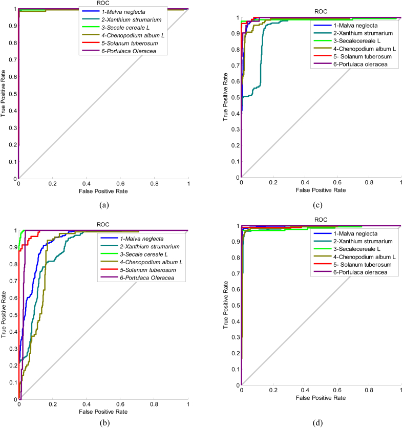
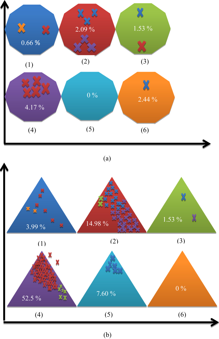
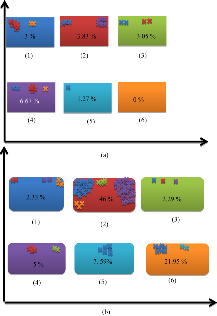
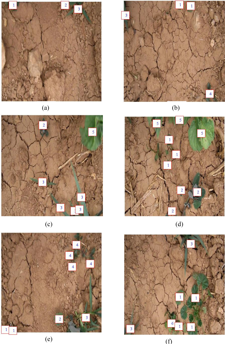
As it was previously mentioned, in order to investigate the performance of classifiers, 959 samples (20% of all data available) are considered as test data. Figure 9 shows the graph of ROC curves for hybrid ANN-CA, LDA, SVM and RF classifiers. As it can be observed on Figure 9, for each class, a curve plot is depicted totaling six different graphs. Horizontal axis of graph is 1-specificity (FP) and its vertical axis represents sensitivity (TP), thus ROC curves are plotted in the plane. As a general rule, the closer graph is to bisector line, the weaker classifier performance in that class is, being bisector line ROC curve the worst case possible of tossing a coin on air to decide whether that object belongs to class or not, with an area under curve (AUC) of 0.5. ROC curves are independent of the number of samples in each class and investigates the performance of classifier only based on the number of samples that are misclassified in that certain class. In Figure 10, class number is shown beneath each color polygon. Class numbers are listed next: 1-Malva neglecta, 2-Xanthium strumarium, 3-Secale cereale L, 4-Chenopodium album L, 5- Solanum tuberosum (Martona potato plant) and 6-Portulaca oleracea. As it can be observed in Figure 10, with hybrid ANN-CA, Xanthium strumarium class has the highest number of error samples while with LDA, Chenopodium album L has the highest number of classification errors, and therefore the AUC for these two classes is lower than that in other classes; Figure 9 proves previous statement where each class ROC is shown with a specific color. Product × sign inside each polygon in Figure 10 shows the number of samples that are wrongly classified. Multiplication sign × color also shows the class color code where sample is wrongly classified in. For example, first polygon of Figure 10(a) has two product × signs in orange and red color; this implies that one sample of Malva neglecta is wrongly classified in Xanthium strumarium and another one misclassified in Portulaca oleracea class. The numbers inside each polygon show the level of prototype classifier error in identifying the samples belonging to each class. For example, in Figure 10(b) in class 4-Chenopodium album L, the number 52.5% is shown implying that value of misclassification rate in LDA classifier for this plant species class. As it can be observed again, statistical LDA does not properly discriminate among similar classes, like Xanthium strumarium and Chenopodium album L. In a similar fashion, misclassifications are also shown apparent for the SVM and RF classifiers, in Figure 11(a) and (b), respectively, where performance of the RF method is quite good as compared to SVM and LDA but still behind that of ANN-CA. Finally, by observing both Figures 9, 10, and 11 the superiority of hybrid ANN-CA method over others is clear, closely followed by RF. In order to understand the efficiency of machine vision prototype, six sample frames of weed plant identification video processing are shown in Figure 12. In this figure, plant class numbers again correspond to: 1-Malva neglecta, 2-Xanthium strumarium, 3-Secale cereale L, 4-Chenopodium album L, 5-Marfona potato plant (Solanum tuberosum) and 6-Portulaca oleracea. As it can be observed, proposed machine vision weed plant detection and classification prototype in potato field is able to properly identify the various kinds of plant inside each video frame.
Figure 9.
ROC curves for the six plant species and both machine learning approaches, over the test set. (a): ANN-CA {ANN-CA.fig}, (b): LDA {LDA.fig}, (c): SVM {ROC_SVM.fig}, and (d): RF {ROC_Randomforest.fig}. Note: Corresponding interactive Matlab .fig file names, are indicated between brackets. Plant class numbers: 1-Malva neglecta, 2-Xanthium strumarium, 3-Secalecereale L, 4-Chenopodium album L, 5-Solanum tuberosum (Marfona potato plant) and 6-Portulaca oleracea.
Figure 10.
Classification system error in each class, (a): hybrid ANN-CA classifier, (b): LDA classifier, Classes are marked with a specific color from one to six. Plant class numbers: 1-Malva neglecta, 2-Xanthium strumarium, 3-Secalecereale L, 4-Chenopodium album L, 5-Solanum tuberosum (Marfona potato plant) and 6-Portulaca oleracea.
Figure 11.
Classification system error in each class, (a): RF classifier, (b): SVM classifier. Classes are marked with a specific color from one to six. Plant class numbers: 1-Malva neglecta, 2-Xanthium strumarium, 3-Secalecereale L, 4-Chenopodium album L, 5-Solanum tuberosum (Marfona potato plant) and 6-Portulaca oleracea.
Figure 12.
Six video frame examples (a) {1.fig}, (b) {2.fig}, (c) {3.fig}, (d) {4.fig}, (e) {5.fig}, and (f) {6.fig}, of the proposed machine weed video detection and classification system. Note: Corresponding interactive Matlab .fig file names, are indicated in brackets. Each video frame incudes class number of plant species: Plant class numbers: 1-Malva neglecta, 2-Xanthium strumarium, 3-Secalecereale L, 4-Chenopodium album L, 5-Solanum tuberosum (Marfona potato plant) and 6-Portulaca oleracea.
Since the method here proposed is new and applied to an unpublished video database, there is no possibility for direct comparison with results previously published. Nevertheless, results presented here were compared with results of two studies in the literature that used different methods for identifying weed. Table 10 compares the success rate of here proposed prototype with two other methods in classifying crop and weeds. The first method is described in Pantazi et al. (2016) that classified 10 types of weeds using hyper-spectral images. They classified weeds using four classifiers and best results of classification were found in Gaussian mixture method. As it can be observed from Table 10, 134 samples were wrongly classified among 540 total samples, resulting in a CCR of 75.19%. Second method to compare with is described in Hlaing and Khaing (2014). They classified four weed types, Rape plant, Lanchon, Falcaria vulgaris and Kyautkut, using an area thresholding algorithm. As it is shown in Table 10, among a total of 35 weed samples, 6 samples were misclassified resulting in a CCR of 82.86%. As it can be observed, the suggested method with more number of samples has higher CCR in identifying weeds than its partners, despite a direct comparison is not possible for obvious reasons. After analyzing the performance of the proposed machine video processing prototype, it is shown that is able to properly identify Marfona potato plant (Solanum tuberosum) among five weed plants (Malva neglecta, Xanthium strumarium, Secale cereale L, Chenopodium album L, and Portulaca oleracea) at a processing speed up to 0.15 m/s with an accuracy of 98%, over the test set.
Table 10.
Correct classification rate comparison of proposed method (ANN-CA) with two examples in the literature on classification of crops and weed. Note: please note the databases used are different in each case, so a valid direct numerical comparison is not possible.
| Method | Total number of samples | Number of invasive plant species | Number of misclassified plant samples | Correct classification rate (%) |
|---|---|---|---|---|
| Proposed prototype | 959 (test set) | 5 | 16 (ANN-CA) | 98.33 |
| Pantazi et al. (2016) | 540 | 10 | 134 (Gaussian) | 75.19 |
| Hlaing and Khaing (2014) | 35 | 4 | 6 | 82.86 |
3.4. Prototype video weed plant detection examples
For illustrative purposes, we include next a total of six segmented and un-segmented (three un-segmented original recording, three segmented and classified) mp4 format videos of around one minute time duration each: three un-segmented videos for reproducible and potential future comparison experiments (SV4, SV5 and SV6) and three video detection and classification segmented examples (SV1, SV2 and SV3), where in the latter case class labels (either numbers or symbols) are apparent, as output from the proposed automatic video weed detection, segmentation and classification prototype in the visible range in Marfona potato field, where one can see how the proposed prototype works under real environment conditions in the on-the-fly discrimination between the following plant species, Marfona potato plant and five weed species:
-
1.
Malva neglecta (mallow)
-
2.
Portulaca oleracea (purslane)
-
3.
Chenopodium album L (lamb's quarters)
-
4.
Secale cereale L (rye)
-
5.
Solanum tuberosum (Marfona potato plant)
-
6.
Xanthium strumarium (cocklebur)
4. Conclusions
The goal was to introduce a visible-range novel, automatic and accurate video processing machine vision system and meta-heuristic classifier prototype in potato plant identification and classification of five weed under real environment potato field conditions, comprising 1-Malva neglecta, 2-Xanthium strumarium, 3-Secale cereale L, 4-Chenopodium album L, 5- Solanum tuberosum (Marfona potato plant) and 6-Portulaca oleracea. Results showed that using the proposed prototype, classification of potato plant and weed with an overall accuracy of 98% over the test set is possible. Main results shown here are summarized next to conclude:
-
1.
Using meta-heuristic methods showed to be accurate for extracting effective discriminant features in our problem at hand. Among three hybrid artificial neural network feature selection methods considered, ANN-ACO, ANN-SA and ANN-GA, last one selected the most effective features.
-
2.
Color features had an important role in classification in our problem at hand. Among six selected features by hybrid ANN-GA, four features are indeed color features: standard deviation of saturation (S) component in HSV color space, mean value of hue (H) component in HSI color space, mean blue-difference chrominance (Cb) component in YCbCr color space, and standard deviation of in-phase (I) component in YIQ color space.
-
3.
LDA statistical methodology has shown weaknesses in proper classification in our video frame object database and problem at hand. For comparison purposes, LDA and hybrid ANN-CA correctly classified samples in Chenopodium album L with only a 47.5% and 95.83% CCR, respectively, over the test set. RF has also shown very nice classification performance in a consistent fashion among the various weed plants.
To conclude, it is known that a proper time gap in order to recognize and identify all five type weeds considered here, would be about five weeks after planting of potato plants took place, since studied weeds grow within this time frame gap approximately. As further work, it remains open to evaluate and analyze the quality and speed of potato plant growth after site-specific spraying in comparison with the non-spraying counterpart, in order to measure plant growth optimization and increase in Marfona potato plant yield.
Declarations
Author contribution statement
Sajad Sabzi, Yousef Abbaspour-Gilandeh, Juan Ignacio Arribas: Conceived and designed the experiments; Performed the experiments; Analyzed and interpreted the data; Contributed materials, analysis tools or data; Wrote the paper.
Funding statement
This work was supported in part by MINECO under grant number RTI2018-098958-B-I00, Spain, and by the European Union (EU) under Erasmus+ project entitled Fostering Internationalization in Agricultural Engineering in Iran and Russia [FARmER] with grant number 585596-EPP-1-2017-DE-EPPKA2-CBHE-JP.
Competing interest statement
The authors declare no conflict of interest.
Additional information
No additional information is available for this paper.
Contributor Information
Yousef Abbaspour-Gilandeh, Email: abbaspour@uma.ac.ir.
Juan Ignacio Arribas, Email: jarribas@tel.uva.es.
Appendix A. Supplementary data
The following is the supplementary data related to this article:
First example of weed detection and classification in Marfona potato plant field video: class labels are defined with cardinal numerical values inside white boxes (Marfona potato plant being number “5”); 62 seconds (mp4 format).
Second example of weed detection and classification in Marfona potato plant field video: class labels are defined with various color basic-shape symbols and acronyms (Marfona potato plant being “cyan star” symbol + Pot acronym); 40 seconds (mp4 format).
Third example of weed detection, classification and segmentation in Marfona potato plant field video: class labels are defined with cardinal numerical values inside white boxes (Marfona potato plant being number “5”) and various plants and weed shapes are also shown segmented (in white); 62 seconds (mp4 format).
First example of weed in Marfona potato plant field original recording un-segmented video; 61 seconds (mp4 format).
Second example of weed in Marfona potato plant field original recording un-segmented video; 58 seconds (mp4 format).
Third example of weed in Marfona potato plant field original recording un-segmented video; 58 seconds (mp4 format).
References
- Abouelatta O.B. Classification of copper alloys microstructure using image processing and neural network. J. Am. Sci. 2013;9(6):213–222. [Google Scholar]
- Ali M.Z., Awad N.H., Suganthan P.N., Duwairi R.M., Reynolds R.G. A novel hybrid Cultural Algorithms framework with trajectory-based search for global numerical optimization. Inf. Sci. 2016;334:219–249. [Google Scholar]
- Banerjee P., Bhunia A.K., Bhattacharyya A., Roy P.P., Murala S. Local Neighborhood intensity pattern - a new texture feature descriptor for image retrieval. Expert Syst. Appl. 2018;113:100–115. [Google Scholar]
- Bhattacharyya A., Saini R., Roy P.P., Dogra D.P., Kar S. recognizing gender from human facial regions using genetic algorithm. Soft Computing. 2018;23:8085–8100. [Google Scholar]
- Dahinden Corinne, Ethz M.A.T.H. vol. 1. 2011. An improved Random Forests approach with application to the performance prediction challenge datasets; pp. 223–230. (Hands-on Pattern Recognition, Challenges in Machine Learning). [Google Scholar]
- Dash A.K., Behera S.K., Dogra D.P., Roy P.P. Designing of marker-based augmented reality learning environment for kids using convolutional neural network architecture. Displays. 2018;25:46–54. [Google Scholar]
- Devijver P.A., Kittler J. Prentice-Hall; London, U.K.: 1982. Pattern Recognition: a Statistical Approach. [Google Scholar]
- Eyre M.D., Critchley C.N.R., Leifert C., Wilcockson S.J. Crop sequence, crop protection and fertility management effects on weed cover in an organic/conventional farm management trial. Eur. J. Agron. 2011;34:153–162. [Google Scholar]
- Fisher R.A. The use of multiple measurements in taxonomic problems. Annal. Eugenics. 1936;7(2):179–188. [Google Scholar]
- Garg H. A hybrid PSO-GA algorithm for constrained optimization problems. Appl. Math. Comput. 2016;274:295–305. [Google Scholar]
- Gianessi L.P., Reigner N.P. The value of herbicides in U.S. crop production. Weed Technol. 2007;21(2):559–566. [Google Scholar]
- Gonzalez R.C., Woods R.E., Eddins S.L. Prentice Hall; 2004. Digital Image Processing Using Matlab. [Google Scholar]
- Guerrero J.M., Pajares G., Montalvo M., Romeo J., Guijarro M. Support Vector Machines for crop/weeds identification in maize fields. Expert Syst. Appl. 2012;39:11149–11155. [Google Scholar]
- Hamuda E., Glavin M., Jones E. A survey of image processing techniques for plant extraction and segmentation in the field. Comput. Electron. Agric. 2016;125:184–199. [Google Scholar]
- Hlaing S.H., Khaing A.S. Weed and crop segmentation and classification using area thresholding. Int. J. Renew. Energy Technol. 2014;3(3):375–382. [Google Scholar]
- Horning Ned. vol. 911. 2010. Random forests: an algorithm for image classification and generation of continuous fields data sets. (Proceedings of the International Conference on Geoinformatics for Spatial Infrastructure Development in Earth and Allied Sciences, Osaka, Japan). [Google Scholar]
- Jayasinghe L., Wijerathne N., Yuen C., Zhang M. Feature Learning and Analysis for Cleanliness Classification in Restrooms. IEEE Access. Jan 2019;7:14871–14882. [Google Scholar]
- Kazmi W., Garcia-Ruiz F.J., Nielsen J., Rasmussen J., Andersen H.J. Detecting creeping thistle in sugar beet fields using vegetation indices. Comput. Electron. Agric. 2015;112:10–19. [Google Scholar]
- Kim J.H., Kim B.G., Roy P.P., Jeong D.M. Efficient facial expression recognition algorithm based on hierarchical deep neural network structure. IEEE Access. 2019;7:41273–41285. [Google Scholar]
- Lin P., Contreras M.A., Dai R., Zhang J. A multilevel ACO approach for solving forest transportation planning problems with environ constraints. Swarm Evol. Comput. 2016;28:78–87. [Google Scholar]
- Marques O. John Wiley & Sons, Inc; Hoboken, New Jersey: 2011. Practical Image and Video Processing Using Matlab. [Google Scholar]
- Mukherjee S., Saini R., Kumar P., Roy P.P., Dogra D.P., Kim B.G. Fight detection in hockey videos using deep network. J. Multimed. Inf. Syst. 2017;4(4):225–232. [Google Scholar]
- Mukherjee S., Kumar P., Saini R., Roy P.P., Dogra D.P., Kim B.G. Plant disease identification using deep neural networks. J. Multimed. Inf. Syst. 2017;4(4):233–238. [Google Scholar]
- Pantazi X.-E., Moshou D., Bravo C. Active learning system for weed species recognition based on hyperspectral sensing. Biosyst. Eng. 2016;146:193–202. [Google Scholar]
- Papamichail D., Eleftherohorinos I., Froud-Williams R., Gravanis F. Critical periods of weed competition in cotton in Greece. Phytoparasitica. 2002;30:105–111. [Google Scholar]
- Shidnal S. A texture feature extraction of crop field images using GLCM approach. Int. J. Sci. Eng. Adv. Tecnol. 2014;2:1006–1011. [Google Scholar]
- Sudeep K.M., Amarnath V., Pamaar A.R., De K., Saini R., Roy P.P. Tracking players in broadcast sports. J. Multimed. Inf. Syst. 2018;5(4):257–264. [Google Scholar]
- Tang J.L., Chen X.Q., Miao R.H., Wang D. Weed detection using image processing under different illumination for site-specific areas spraying. Comput. Electron. Agric. 2016;122:103–111. [Google Scholar]
- Wisaeng K. A comparison of decision tree algorithms for UCI repository classification. Int. J. Eng. Trends Technol. 2013;4:3393–3397. [Google Scholar]
- Yang M.H., Ahuja N. Vol. 1. Hilton Head Island, June; 2000. A geometric approach to train support vector machines; pp. 430–437. (Proceedings of the 2000 IEEE Conference on Computer Vision and Pattern Recognition). [Google Scholar]
- Yang X., Tridandapani S., Beitler J.J., Yu D.S., Yoshida E.J., Curran W.J., Liu T. Ultrasound GLCM texture analysis of radiation-induced parotid-gland injury in head-and-neck cancer radiotherapy: an in vivo study of late toxicity. Med. Phys. 2012;39(9):5732–5739. doi: 10.1118/1.4747526. [DOI] [PMC free article] [PubMed] [Google Scholar]
- Zameer A., Mirza S.M., Mirza N.M. Core loading pattern optimization of a typical two-loop 300 MWe PWR using Simulated Annealing (SA), novel crossover Genetic Algorithms (GA) and hybrid GA(SA) schemes. Ann. Nucl. Energy. 2014;65:122–131. [Google Scholar]
- Zimdahl R.L. Academic Press; San Diego, CA, USA: 1993. Fundamentals of weed Science. [Google Scholar]
Associated Data
This section collects any data citations, data availability statements, or supplementary materials included in this article.
Supplementary Materials
First example of weed detection and classification in Marfona potato plant field video: class labels are defined with cardinal numerical values inside white boxes (Marfona potato plant being number “5”); 62 seconds (mp4 format).
Second example of weed detection and classification in Marfona potato plant field video: class labels are defined with various color basic-shape symbols and acronyms (Marfona potato plant being “cyan star” symbol + Pot acronym); 40 seconds (mp4 format).
Third example of weed detection, classification and segmentation in Marfona potato plant field video: class labels are defined with cardinal numerical values inside white boxes (Marfona potato plant being number “5”) and various plants and weed shapes are also shown segmented (in white); 62 seconds (mp4 format).
First example of weed in Marfona potato plant field original recording un-segmented video; 61 seconds (mp4 format).
Second example of weed in Marfona potato plant field original recording un-segmented video; 58 seconds (mp4 format).
Third example of weed in Marfona potato plant field original recording un-segmented video; 58 seconds (mp4 format).


