Using a 22-Layer U-Net to Perform Segmentation of Squamous Cell Carcinoma on Digitized Head and Neck Histological Images

Abstract

Squamous cell carcinoma (SCC) comprises over 90 percent of tumors in the head and neck. The diagnosis process involves performing surgical resection of tissue and creating histological slides from the removed tissue. Pathologists detect SCC in histology slides, and may fail to correctly identify tumor regions within the slides. In this study, a dataset of patches extracted from 200 digitized histological images from 84 head and neck SCC patients was used to train, validate and test the segmentation performance of a fully-convolutional U-Net architecture. The neural network achieved a pixel-level segmentation AUC of 0.89 on the testing group. The average segmentation time for whole slide images was 72 seconds. The training, validation, and testing process in this experiment produces a model that has the potential to help segment SCC images in histological images with improved speed and accuracy compared to the manual segmentation process performed by pathologists.

INTRODUCTION

Squamous cell carcinoma (SCC) of the head and neck is one of the most common forms of cancer and over 500,000 cases of head neck SCC are reported worldwide each year [1]. Medical studies also indicate that SCC of the head and neck is often preventable and even curable if diagnosed early [1]. The diagnosis process for SCC generally involves constructing histology slides from extracted tissue samples and detecting regions of SCC within these slides. Due to the fact that early diagnosis is critical to curing cases of SCC and pathologists may make interpretive errors when attempting to detect SCC, machine learning techniques for medical image segmentation have the potential to benefit both pathologists and SCC patients by aiding in the diagnosis process.

Previously, several fully convolutional neural network architectures, including U-Net, have been successfully applied to a wide variety of medical image segmentation tasks ranging from cell-nuclei segmentation to prostate cancer segmentation [2, 3, 4]. For example, the study that first introduced the U-Net architecture reported an IOU (intersection over union) of about 0.92 for a particular dataset from the 2015 ISBI Cell Tracking Challenge [2]. In addition, a recent study implemented fully convolutional architectures based on U-Net and ResNet to achieve an average AUC over 0.8 for a prostate cancer segmentation task using MRI images [3].

Our previous work focused on using a patch-based Inception V4 CNN to detect SCC using a dataset of 192 digitized histological images from 84 head and neck SCC patients [5]. The method we proposed in the previous work achieved an AUC of 0.91 on the testing group and an AUC of 0.92 on the testing group.

The goal of this study is to evaluate the ability of fully-convolutional neural networks such as U-Net to perform cancer segmentation of SCC in digitized histological images of the head and neck. While the previous study used this dataset to train a CNN to perform patch-level SCC classification, this study focuses on the arguably more difficult problem of SCC segmentation, which generates class labels at the pixel-level. This study also uses a fully-convolutional network that is fundamentally different from the fully-connected Inception V4 CNN used in the previous paper, and yields a method that not only detects SCC at the patch-level, but also identifies exact SCC regions within histological images with pixel-level resolution. While the U-Net architecture has been applied to a wide variety of tasks including cell-nuclei detection and even CT lung segmentation [6], a recent literature review suggests that this study is perhaps the first to investigate the application of U-Net specifically for the task of head and neck SCC segmentation. The robust experimental design and preliminary results of this study demonstrate that this method has the potential to aid pathologists in performing cancer segmentation of SCC in head and neck histological images with improved accuracy through a model that can segment an average slide in a matter of seconds.

METHODOLOGY AND APPROACH

Data Source: Head and Neck SCC Patient Tissue Samples

As part of a joint effort with the Otolaryngology Department and the Department of Pathology and Laboratory Medicine at Emory University Hospital Midtown, ex-vivo tissue examples were collected from consented patients undergoing surgical cancer resection [7, 8]. For each patient, three different tissue samples were collected. The first tissue sample was extracted from a region of all tumor tissue, the second sample consisted of all normal tissue, and the third sample was extracted at the boundary between the normal and tumor tissue regions. In total, 200 tissue samples from 84 head and neck SCC patients were used and divided into separate sets for training U-Net, validating its performance, and testing its performance at the very end. The training set consisted of 105 slides extracted from 45 different patients, while the validation set consisted of 29 slides extracted from a different set of 13 patients. After optimizing the CNN on the training set and evaluating its generalization ability using the validation set, a separate testing set of 66 slides obtained from 26 new patients was used to provide a final statistical evaluation of the CNN’s performance. This testing set was not employed until the end of the experiment in order to ensure that the final results provided an unbiased measurement of the CNN’s ability to generalize to unseen data.

Histological Processing and Patch-Based Dataset

The dataset used to implement the U-net architecture was a digitized H&N SCC dataset we previously reported [5]. The histology slide images were prepared using a standard procedure, where the tissue samples were fixed, embedded in paraffin, sectioned, and stained with haemotoxylin and eosin, and finally digitized using whole-slide scanning. In order to provide a labeled ground truth for the training, validation, and testing examples, a certified pathologist (James V. Little), outlined the cancer regions on the digital slides using Aperio ImageScope (Leica Biosystems Inc, Buffalo Grove, IL, USA). As outlined in the previous subsection, the data was split into separate training, validation and testing sets. Each slide was accompanied by a binary segmentation mask in matrix form indicating the regions of cancer and normal tissue. The slides were also down-sampled by a factor of four, and 512 × 512 pixel patches were extracted from the down-sampled slides to produce the final training, validation, and testing sets used to train and evaluate the CNN. The final training dataset used to train the CNN consisted of about 30,747 patches. Originally, the dataset consisted of far fewer patches from margin slides and from normal tissue slides, but additional patches from both groups were produced using data augmentation in the form of vertical and horizontal flips. The validation and test datasets consisted of 13,511 and 38,659 patches respectively (Table 1, Figure 2).

Table 1:

Tumor (T), normal (N), and tumor-normal (TN) whole slide images (WSI) and patches in each dataset.

Dataset	Patients	T (WSI)	TN (WSI)	N (WSI)	T (Patches)	TN (Patches)	N (Patches)	Total (WSI)	Total (Patches)
Training	45	34	37	34	10929	11244	8574	105	30747
Validation	13	4	17	8	2621	7720	3170	29	13511
Testing	26	24	20	22	8853	24726	5080	66	38659

Figure 2:

Modified U-Net architecture with 22 convolutional layers.

Fully Convolutional U-Net Architecture

The dataset discussed in the previous section was used to train, validate, and test a 2D fully-convolutional CNN based largely on the original U-Net architecture. The CNN was implemented using Keras, a high-level machine learning library that uses TensorFlow as a backend, and trained on a 1080Ti NVIDIA GPU [9–10]. The CNN was trained using a relatively small batch size of 4 patches and batch normalization after each activation layer. Several techniques were used to add regularization and improve the CNN’s generalization ability. Batch-based data augmentation, in which the hue, saturation, brightness, and contrast of each patch was randomly modified, was implemented to allow the network to learn invariance to these features. After applying these transformations each batch of patches was converted from the RGB space to the HSV space before being processed by the CNN during each gradient step. One of the advantages of using the HSV image representation for training the CNN is that this representation separates color information from intensity information without the CNN having to learn this separation of features from the RGB image representation. In order to provide additional forms of regularization to minimize overfitting, L2-regularization with an L2 constant of 10⁻⁷ was applied to the loss function for each convolutional layer and a dropout ratio of 5% plied after each block of convolutional layers [11–12]. The architecture for the CNN was based on the original U-Net architecture, but contained 22 standard convolutional layers organized into 11 convolutional blocks as opposed to the original architecture, which only contained 18 standard convolutional layers organized into 9 convolutional blocks [1]. Additional convolutional blocks were used in order to produce a model with more learnable parameters that could generalize better to a more complex problem. In comparison, our previous work used a much deeper and more computationally-expensive, patch-based Inception V4 CNN with 141 standard convolutional layers. The Inception V4 CNN also used much smaller 101 × 101 pixel patches for training. Even with far less convolutional layers and a larger patch size, the CNN used in this paper is still able to learn a more complex task that yields a pixel-level segmentation map for each patch rather than a single class label for each patch.

The CNN was optimized using the Adadelta optimizer with an initial learning rate of 1.0 and was trained for only two epochs due to the large size of the extensively augmented training dataset [13]. For the loss function, we used a pixel-by-pixel sum of the cross entropy for each pixel over the final predicted probabilities ${\widehat{p}}_i$ and the ground truth values p_i in the final segmentation map defined in the equation below.

$$L=\sum _i\text{log}\left({\widehat{p}}_i\right)p_i$$

The original U-Net paper used a weighted cross entropy loss to account for background pixels, but we used a standard cross entropy loss due to the absence of background pixels in our training patches. While our loss function was similar to the one that the original U-Net paper reported [2], we used the Adadelta optimizer rather than the stochastic gradient descent optimizer used in the original paper. One advantage of using the Adadelta algorithm for optimization is that it uses adaptive learning rates rather than a fixed learning rate in the case of stochastic gradient descent, allowing for faster convergence. The use of only two epochs to train our network can be justified by the use of heavy data augmentation along with the fast convergence achieved by Adadelta. To achieve comparable results in practice, the constant learning rate for stochastic gradient descent (SGD) must be carefully tuned manually through experimentation, which can be quite time consuming. The Adadelta algorithm, for which we used a decay rate of ρ = 0.9 and a constant of ϵ = 10⁻⁶, is described in Algorithm 1 below [13].

Based on the procedure above, the Adadelta algorithm accumulates a weighted sum of the gradients over a fixed window as well as the weight updates. Each weight update is computed using a changing “learning rate” that is essentially the ratio of the root mean square (RMS) of the accumulated weight updates and the RMS of the accumulated gradient values. The RMS statistic refers the square-root of the arithmetic mean of the squares of a sequence of values (x_i), as defined in the equation below.

$$\text{RMS}(x)=\sqrt{\frac{{\sum }_{i=1}^n{x}_i^2}{n}}$$

This adaptive learning rate eliminates the need to carefully select a starting learning rate and a learning rate schedule, which is often required for comparable performance when working with non-adaptive optimization such as stochastic gradient descent. In addition, because Adadelta takes into account the past weight updates, a separate adaptive learning rate is used for each parameter in the network during each weight update [13]. This property allows for the earlier layers with smaller gradients in the network to be updated with larger learning rates and later layers with larger gradients to be updated with smaller learning rates, which can allow the optimization process to converge earlier.

RESULTS

The U-Net architecture was able to perform SCC segmentation on digitized histological images with a pixel-level AUC of 0.89 for patients in the testing group (Table 2). Based on the AUC and corresponding receiver operator characteristic (ROC) curve for the validation data, the optimal probability threshold for distinguishing an SCC tumor region from a region of normal tissue was determined to be 0.2845. This threshold was applied to both the validation and testing sets to produce the accuracy, sensitivity, and specificity for each set. Three sample validation slides are classified and presented using probability heat maps in Figure 3 to demonstrate the segmentation performance of the CNN. As far as classification speed is concerned, the proposed method in this paper produces an output for a given histological slide faster than the method in our previous paper. The Inception V4 CNN in our previous paper classified whole slide images in an average time of 7 minutes with a standard deviation of 9 minutes, while the U-Net CNN in this paper segmented whole slide images in an average time of only 72 seconds with a standard deviation of 43 seconds.

Table 2:

SCC segmentation results at the pixel-level across the whole dataset for the validation and testing sets.

Dataset	Slides	Patches	AUC	Accuracy	Sensitivity	Specificity
Validation	35	13,511	0.80	74%	69%	78%
Testing	66	38,659	0.89	82%	81%	82%

Figure 3:

The Adadelta algorithm used for optimizing the CNN [13].

In Table 2, the sensitivity or true positive rate, and the specificity, or true negative rate, are computed using the equations below.

$$\mathit{\text{Sensitivity}}=\frac{TP}{TP+FN}$$

$$\mathit{\text{Specificity}}=\frac{TN}{TN+FP}$$

Where TP, FP, TN and FN represent the number of true positives, false positives, true negatives, and false negatives respectively.

The difference in performance on the validation and testing sets can be explained by the difference in the size and composition between the two sets. The validation set contains far fewer patches than the testing set and may not be as well representative of the population for this problem as the test set. While the testing set contains a roughly balanced number of tumor, tumor-normal, and normal whole-slide images, the validation set does not (Table 1). The specificity on the validation set is notably higher than the sensitivity but the two metrics are similar for the testing set, perhaps due to the larger size and more representative nature of the testing set. When interpreting the results, the testing results are, as expected, likely a better measurement of the CNN’s segmentation performance on large samples of unseen slides.

DISCUSSION

In this study, we present an extensive dataset of digitized histological slides of head and neck SCC and implement a version of the U-Net architecture for SCC segmentation. To the best of our knowledge, this is the first work to investigate the application of fully convolutional architectures, such as U-Net, to the task of SCC segmentation in digitized histological images from head and neck SCC cancers. Previously our group worked to use a standard, patch-based CNN using this dataset [5]. While the patch-based CNN achieved a testing AUC of 0.92, our fully convolutional U-Net CNN achieved a testing AUC of 0.89. The difference in the testing AUC between the two CNNs can be explained by the difference in difficulty of the two tasks. We argue that the patch-level SCC detection task performed by the fully-connected patch-level CNN is easier than the pixel-level SCC segmentation task performed by the U-Net CNN in this work. In addition, when using graphical processing units (GPUs), fully-convolutional networks are more computationally efficient than fully-connected CNNs due to the absence of fully-connected layers. Another advantage of the fully-convolutional CNN in this paper is that it produces more precise outputs for an SCC slide by detecting SCC regions at the pixel level, rather than the patch level. The main disadvantage of the fully-convolutional network however is that in order to produce more precise outputs, it requires more precise training data where SCC regions such should be labeled accurately with pixel-level resolution. This level of precision may be more difficult or computationally expensive to obtain. However, if obtaining this data is not an issue, the resulting fully-convolutional CNN will produce more precise and possibly more useful outputs for a histology slide than a fully-connected CNN.

While we chose to apply the commonly used U-Net architecture to the task of SCC segmentation in histological images, we made a few notable modifications to the training procedure described in the paper that introduced the U-Net architecture. For example, we added additional convolutional blocks in order to increase the number of parameters that the network could use to learn this potentially more complex task of SCC segmentation. In order to increase the amount of regularization and prevent overfitting, we also used dropout along with L2 weight regularization in addition to heavy data augmentation. The original U-Net paper mentions the use of data augmentation but not dropout or L2 regularization. A key difference between our training method and the training procedure in the original paper is the use of the Adadelta optimization algorithm as opposed to the SGD algorithm with momentum. Adadelta is an adaptive algorithm that maintains a separate, adaptable learning rate for each parameter in the network and eliminates the need for carefully selecting an initial learning rate and defining a learning rate schedule. This optimization algorithm, along with the use of batch-based random color augmentations, allowed us to achieve convergence in only two epochs.

The application investigated in this paper is also significantly different from the applications described in the first U-Net paper. While this paper investigates the application of U-Net to SCC segmentation in histological images, the original U-Net paper focused on the application of U-Net to various cell-segmentation tasks, some of which are arguably easier than SCC segmentation [2]. Our modifications to the original training procedure, such as the use of additional forms of regularization and a more sophisticated optimization algorithm can be justified by the relative difficulty of the application that we chose to investigate. One of the key challenges that we faced in training the U-Net architecture was constructing the dataset with the right distribution of patches from tumor, normal, and margin slides. Initially, the dataset consisted of thousands of patches from tumor and normal slide samples and only a few hundred patches from margin slides. This issue made it difficult to train the CNN because fully-convolutional architectures for segmentation generally perform well if both classes are present in a significant portion of the training images. There was also a large class imbalance between the tumor and normal patches, with most of the patches in the original dataset corresponding to tumor slides. In order to solve this issue, we increased the number of patches from margin slides artificially using data augmentation and doubled the number of patches from normal slides in order to match the number of tumor patches. This technique, along with the use of random color augmentation and explicit regularization in the form of dropout and L2-regularization terms for each convolutional layer, allowed us to limit overfitting and enable the network to generalize better to unseen validation and testing data.

CONCLUSION

In summary, the proposed method for implementing and training a U-Net architecture yields a CNN that is capable of performing SCC segmentation on digitized histological images of the head and neck with a pixel-level AUC of 0.89 for patients in the validation set. The robust experimental design with separate sets for training, validation, and testing, along with the validation and testing results demonstrate that the CNN is generalizable and is capable of segmenting unseen SCC histological slides with a reasonable level of success.

Figure 1:

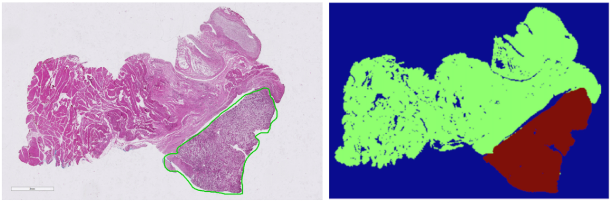
Left: Sample histological slide selected from dataset. Right: Corresponding binary segmentation mask with cancer region outlined in red and normal tissue outlined in green.

Figure 4:

U-Net segmentation results on representative slides from the testing set. Each set of three images contains the original slide image on the left, the correct SCC segmentation in the center, and the CNN’s predictions as a probability heat map on the right. Brighter/warmer areas correspond to higher probabilities of cancer.

REFERENCES

- [1].Marur S, Forastiere AA “Head and Neck Squamous Cell Carcinoma: Update on Epidemiology, Diagnosis, and Treatment”, Proc. Mayo Clinic 91(3), 386–396 (2016). [DOI] [PubMed] [Google Scholar]
- [2].Ronneberger O, Fischer P, Brox T “U-Net: Convolutional Networks for Biomedical Image Segmentation”, Proc. MICCAI, 234–241, (2015). [Google Scholar]
- [3].Chiou E, Giganti F, et al. “Prostate Cancer Classification on VERDICT DW-MRI Using Convolutional Neural Networks”, Proc. Machine Learning in Medical Imaging, 10, 1007, 319–327, (2018). [Google Scholar]
- [4].Kumar Singh V, Rashwan HA, et al. “Breast Mass Segmentation and Shape Classification in Mammograms using Deep Neural Networks”, Proc. CoRR, 1809, 01687 (2018). [Google Scholar]
- [5].Halicek M, Maysam S, et al. , “Head and Neck Cancer Detection in Digitized Whole-Slide Histology Using Convolutional Neural Networks”, Nature Scientific Reports. 9, 14043 (2019). [DOI] [PMC free article] [PubMed] [Google Scholar]
- [6].Skourt BA, Hassani AE, Majda A “Lung CT Segmentation Using Deep Neural Networks”, Proc. ICDS 127, 109–113 (2018). [Google Scholar]
- [7].Fei B, Lu G, Wang X, et al. , “Tumor margin assessment of surgical tissue specimen of cancer patients using label-free hyperspectral imaging,” Proc SPIE Int Soc Opt Eng, 100540E-1, 100540E (2017). [DOI] [PMC free article] [PubMed] [Google Scholar]
- [8].Fei B, Lu G, Wang X, et al. , “Label-free reflectance hyperspectral imaging for tumor margin assessment: a pilot study on surgical specimens of cancer patients,” J Biomed Opt, 22, 7 (2017). [DOI] [PMC free article] [PubMed] [Google Scholar]
- [9].Martín Abadi AA, Barham Paul, Brevdo Eugene, et al. , “TensorFlow: Large-scale machine learning on heterogeneous systems,” https://www.tensorflow.org, (2015).
- [10].Chollet F, Keras, (2015), GitHub repository, https://github.com/keras-team/keras
- [11].Ng. AY, “Feature selection, L 1 vs. L 2 regularization, and rotational invariance.” Proc. ICML, 78, (2004). [Google Scholar]
- [12].Srivastava N, Hinton G, Krizhevsky A, “Dropout: a simple way to prevent neural networks from overfitting.”, Journal of Machine Learning Research, 15(1), 1929–1958 (2014). [Google Scholar]
- [13].Zeiler MD, “ADADELTA: An adaptive learning rate method,” arXiv: Computational Research Repository, 121.5701, (2012).