Selection of Features with Consistent Profiles Improves Relative Protein Quantification in Mass Spectrometry Experiments

Summaries of protein abundance are undermined by mass spectrometric features inconsistent with the overall protein profile. We develop an automated statistical approach that detects such inconsistent features. These features can be separately investigated, curated, or removed. Accounting for such inconsistent features improves the estimation and the detection of differential protein abundance between conditions. The approach is implemented as an option in the open-source R-based software MSstats.

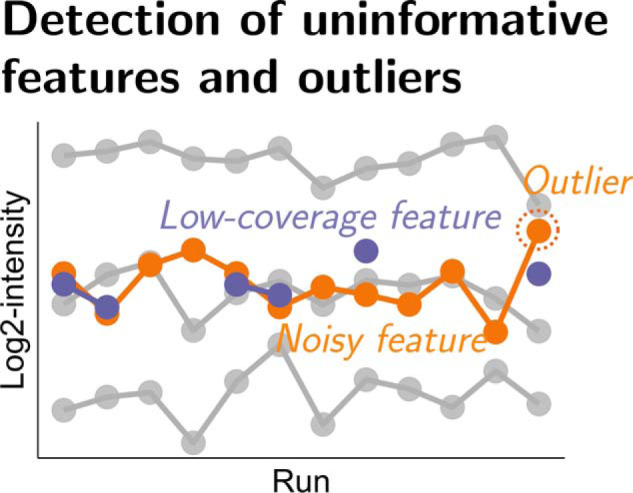
Graphical Abstract

Highlights

• Automated statistical approach for detecting uninformative features and outliers.

• Improved performance on relative protein quantification.

• An option in the open-source R-based software MSstats.

Abstract

In bottom-up mass spectrometry-based proteomics, relative protein quantification is often achieved with data-dependent acquisition (DDA), data-independent acquisition (DIA), or selected reaction monitoring (SRM). These workflows quantify proteins by summarizing the abundances of all the spectral features of the protein (e.g. precursor ions, transitions or fragments) in a single value per protein per run. When abundances of some features are inconsistent with the overall protein profile (for technological reasons such as interferences, or for biological reasons such as post-translational modifications), the protein-level summaries and the downstream conclusions are undermined. We propose a statistical approach that automatically detects spectral features with such inconsistent patterns. The detected features can be separately investigated, and if necessary, removed from the data set. We evaluated the proposed approach on a series of benchmark-controlled mixtures and biological investigations with DDA, DIA and SRM data acquisitions. The results demonstrated that it could facilitate and complement manual curation of the data. Moreover, it can improve the estimation accuracy, sensitivity and specificity of detecting differentially abundant proteins, and reproducibility of conclusions across different data processing tools. The approach is implemented as an option in the open-source R-based software MSstats.

Bottom-up proteomics is a method to analyze peptides from enzymatic digestion of proteins with liquid chromatography coupled with mass spectrometry (LC-MS)¹. It is the most widespread proteomic workflow (2, 3) compatible with data-dependent acquisition (DDA), data-independent acquisition (DIA) (28, 11), and selected reaction monitoring (SRM) (18).

In DDA, the mass spectrometer alternates between acquiring a full MS1 spectrum of the co-eluting precursor ions for analyte quantification and acquiring the fragment MS/MS spectra of the peptide ions for identification. SRM, an important method for targeted analysis, requires an a priori knowledge of the unique peptide sequences of the protein targets. The peptides are selectively profiled based on their precursor ions and representative fragment ions, and quantified by the intensity of each pair of precursor/fragment, also known as transition. Label-based SRM workflows further enhance the accuracy of the quantification by spiking an isotopically labeled reference counterpart of each targeted peptide into the samples. In DIA, the mass spectrometer covers the entire relevant mass range with a set of wide windows. All the precursor ions in a window are co-isolated and subjected to fragmentation, to produce their combined fragment spectrum.

A common use of DDA, SRM and DIA is relative protein quantification. Protein quantification summarizes all the quantitative information pertaining to a protein across the LC-MS runs, and performs statistical analyses that detect differentially abundant proteins between conditions. Because mass spectrometers quantify peptide ions or their fragments instead of proteins, deriving protein-level conclusions can be challenging. First, the quantitative profile of a peptide ion or a fragment can deviate from the representative protein profile for biological reasons (e.g. in presence of post-translational modifications or unknown protein isoforms), or for technological reasons (e.g. because of interferences of co-eluting precursor ions such as ion suppression). Second, some of the precursor ions or fragments can be incorrectly identified or quantified across the LC-MS runs. This is particularly common for low abundant analytes. Third, in DDA workflows, the stochastic nature of the acquisition of fragmentation spectra makes it challenging to consistently identify and measure the same species in multiple LC-MS runs, and produces missing values. Finally, computational processing of the spectra adds uncertainty to protein quantification. A variety of computational tools, e.g. MaxQuant (9, 8), Progenesis (Nonlinear Dynamics, Newcastle upon Tyne, UK), Proteome Discoverer (Thermo Fisher Scientific, Waltham, MA), Skyline (15), DIA Umpire (26), OpenSWATH (20) and Spectronaut (4), identify, quantify and align the peaks across the LC-MS runs. Each tool optimizes different computational tasks, and the resulting list of differentially abundant proteins may be, at least to some extent, tool-dependent. Overall, these issues undermine the accuracy and reproducibility of protein-level summarization and relative quantification.

This manuscript aims to alleviate these challenges. We propose an automated statistical approach, which takes as input a set of identified and quantified spectral features reported by a data processing tool, characterizes the information content in the individual features, and performs relative protein quantification using an informative subset of the features. We consider DDA, SRM and DIA acquisition types, and use the generic term feature to refer to precursor ions in DDA, transitions in SRM, or fragments in DIA, identified and quantified across multiple LC-MS runs. We define informative features as features that contain few missing values, and for which the intensities are consistent with most of the protein intensity profiles across the runs. We define uninformative features as features that do not satisfy these properties. Among those, low-coverage features contain many missing values. Outliers are inconsistent with the overall protein profile. Finally, noisy features exhibit substantial variation between the LC-MS runs, beyond the variation of most of the features of the protein.

Background

Detecting uninformative features in LC-MS data often involves manual curation. A feature of a peptide is evaluated by plotting the proportion of its intensity in the sum of the intensities of all the features of the peptide. For the informative features, this proportion is roughly constant across all the LC-MS runs in the investigation. Deviations from the constant pattern indicate that the feature may be compromised by noise or artifacts and should be further investigated. Such manual curation is limited in throughput. Also, when performed separately for each peptide as in common practice, it does not account for potentially distinct peptide profiles of the same protein.

Automatic approaches for detecting uninformative features have been introduced as alternatives to manual curation. They can be loosely classified into two groups: those detecting interferences or errors in identification and quantification within a single LC-MS run, and those detecting these patterns across multiple LC-MS runs. Many methods consider properties of spectral features in a single LC-MS run. These methods evaluate feature-specific patterns such as relative intensities, chromatographic traces, or patterns of isotopic distributions. The patterns are compared with their expected patterns for the analyte (or, in the case of SRM, to the observed patterns of their isotopically labeled reference counterparts). For example, the scoring model in mProphet (19) combines multiple quality metrics, and filters out peaks with likely incorrect identification, presence of interfering ions, etc. Originally developed for SRM, the mProphet algorithm has since been implemented in Spectronaut, OpenSWATH and Skyline for DIA workflows. Similar steps are implemented in other data processing tools, e.g. SWATHProphet (14) and EncyclopeDIA (21) for DIA.

To select informative features in multiple LC-MS runs, a common heuristic, called “top-n”, selects n features with the highest average intensities across the runs. The heuristic is based on the insight that higher intensity features are less impacted by interference, and therefore have a higher information content. More recent approaches make more sophisticated considerations. For SRM, AuDIT (1) calculates the intensity ratio between each pair of features (i.e. transitions) generated from a same precursor in all runs, compares them to the ratios of the isotopically labeled reference counterparts, and flags significantly deviating ratios using the t test. Although the method is simple and performs well, it requires high-quality information from the standards. For DIA, mapDIA (25) implements a suite of data processing steps, including intensity normalization, fragment filtering, and detection of differentially abundant proteins. The fragment filtering step includes outlier detection and uses pairwise correlation to select features with consistent profiles across the runs. The step is tightly integrated with the rest of the mapDIA workflow and requires tuning multiple parameters that control the cross-fragment correlation and the number of peptides and fragments. Using several quality metrics, Avant-garde (27) automatically curates features with a genetic algorithm and adjusts their peak boundaries for quantification. The method is integrated as an external tool of Skyline. Diffacto (29) performs protein summarization through robust factor analysis of the features, views the features corresponding to the majority factor as representative of the protein, but does not select a subset of informative features.

This manuscript aims to improve upon the existing methods above. We propose a statistical approach that takes as input the identified and quantified features that pass single-run filtering criteria (e.g. by mProphet), and complements the filtering using the information available from multiple LC-MS runs. It selects a subset of informative spectral features for detecting differentially abundant proteins. The uninformative features can be separately investigated, curated, or removed. The approach is compatible with multiple data acquisition workflows and data processing tools.

EXPERIMENTAL PROCEDURES

The input data sets are briefly described below and summarized in Tables I and II. The data sets are available on either MassIVE.quant (5) or Panorama (23). Details about data processing, R script for statistical analysis, and the differential abundance analysis results are available on MassIVE.quant. Data set identifiers and reanalysis container identifiers on MassIVE.quant are listed in Tables I and II. Additionally, the R script for summarizing all the analysis results in this manuscript is available at https://github.com/tsunghengtsai/MSstats-feature-selection.

Table I. Summary of the experimental data sets of benchmark-controlled mixtures.

Benchmark (MassIVE ID)	Evaluation	No. of conditions	No. of runs	Data processing	No. of proteins	Median no. of features per protein	MassIVE reanalysis ID (A = All-features, S = Proposed or top-n)
DDA Choi [7] (MSV000084181)	True FC	5	15	MaxQuant	1549	10	A: RMSV000000261
				Progenesis	1330	9	S: RMSV000000263
				Proteome Discoverer	1271	8
				Skyline	1244	5
DDA iPRG [6] (MSV000079843)	True FC	4	12	MaxQuant	2875	7	A: RMSV000000249
				Progenesis	3015	3	S: RMSV000000259
				Skyline	3027	7
DIA Bruderer [4] (MSV000081828)	True FC	7	21	DIA Umpire	3611	25	A: RMSV000000252
				Skyline	3076	29	S: RMSV000000258
				Spectronaut	3134	33
DIA Navarro [16] (MSV000081024)	True FC	2	6	DIA Umpire	4383	18	A: RMSV000000250
				OpenSWATH	5376	23	S: RMSV000000257
				Skyline	5387	24
				Spectronaut	5486	13

Table II. Summary of the experimental data sets from biological investigations. Data from the investigation by Dunkley et al. are available on Panorama (https://panoramaweb.org/neuroSRM.url).

Investigation (MassIVE ID)	Evaluation	No. of conditions	No. of runs	Data processing	Feature_q-filter	No. of proteins	Median no. of features per protein	MassIVE reanalysis ID (A = All-features, S = Proposed or top-n)
DIA Selevsek [22] (MSV000081677)	Low-CV analysis	6	18	Skyline	Full_Sparse	2189	24	A: RMSV000000251
					Full_50%	1821	24	S: RMSV000000262
					LowCV_Sparse	2212	24
					LowCV_50%	2204	24
SRM Dunkley [10]	Manual curation	10	95	Skyline	Full	246	6

Benchmark Controlled Mixtures

We evaluated the proposed approach on four benchmark-controlled mixtures of known composition. Raw spectra from a same investigation were processed with up to four data processing tools. Data from two controlled mixtures were acquired with DDA: (1) the iPRG benchmark (6), where the data were processed by MaxQuant, Progenesis, and Skyline; and (2) the Choi benchmark (7), where the data were processed by MaxQuant, Progenesis, Proteome Discoverer, and Skyline. Data from two controlled mixtures were acquired with DIA: (1) the Bruderer benchmark (4), where the data were processed by DIA Umpire, Skyline, and Spectronaut; and (2) the Navarro benchmark (16), where the data were processed by DIA Umpire, OpenSWATH, Skyline, and Spectronaut.

This work did not aim to compare the data processing tools. Rather, we used these data sets to evaluate the impact of the proposed approach on accuracy of fold-change estimation, sensitivity and specificity of detecting differentially abundant proteins, and reproducibility of conclusions across the data processing tools. We compared the performance to (1) all-features protein quantification, as currently implemented in MSstats, and (2) protein quantification based on the n features with the highest average intensities across runs (i.e. top-n features) using MSstats.

Biological Investigations

We evaluated the proposed approach using two biological investigations. The first is a label-based SRM experiment by Dunkley et al. (10), investigating in vivo neuro-development. In addition to the biological samples, the experiment included 35 replicate runs from a pooled quality control (QC) sample to assess the technical performance. Also, spike-in experiments with pooled isotope-labeled peptides spiked into the QC sample were performed to characterize the linear portion of the dynamic range for each analyte. The data were processed with Skyline, and the quality of each feature was manually curated. The manual curation consisted of two steps: (1) removing peptides with no signal, and transitions with interference, and (2) removing peptides that failed to meet a set of thresholds based on coefficient of variation (CV) of the QC runs, and the range of intensity values compared with the linear portion of the dynamic range. Whenever either an endogenous or a reference feature did not meet the quality thresholds, the entire pair was removed. Further details regarding the manual curation can be found in (10). We used this data set to evaluate the capability of the proposed approach to automatically detect uninformative features, as compared with the manual curation.

The second biological investigation is a DIA-based experiment by Selevsek et al. (22). The main investigation quantified the proteome of Saccharomyces cerevisiae in response to osmotic stress at six time points. In addition, a separate refinement experiment performed eight technical DIA runs on a same biological sample. Two analyses of the resulting data were performed in the study, both using Skyline. The first analysis, which we call Full, considered all the peptide precursors in the main investigation, and quantified each precursor with the top-6 fragments. The second analysis, which we call LowCV, selected peptides detected in at least 50% of the refinement runs, and with CV < 20% in those runs. The selected peptides were then quantified in the biological samples in the main investigation. After these steps, the features selected in both analyses were further subjected to mProphet to characterize the quality of the peaks in individual LC-MS runs in terms of q-values. Compared with the Full analysis, the LowCV analysis queried against a reduced spectral library. Therefore, a peak in the two analyses could have different q-values. We considered two types of q-filters: i) the Sparse q-filter eliminated peaks with q-value > 0.01, and ii) the 50% q-filter eliminated the entire LC-MS features where the q-values of over 50% of the peaks exceeded 0.01. Combinations of the two data analyses with the two q-filter strategies produced four data sets: Full_Sparse, Full_50%, LowCV_Sparse, and LowCV_50%. We used these data sets to evaluate the impact of the proposed approach on relative protein quantification under different choices of data processing. All the downstream statistical analyses were performed with MSstats v3.16.2.

Simulated Data Sets

In addition to the experimental data, computer simulations evaluated the effect of outliers, and of different number of features and runs, on the performance of the proposed approach. The details are in supplementary Section S1.

Proposed Statistical Approach for Selecting Informative Features

Overview and Notation

The input to the approach is a list of log-transformed intensities (peak areas, heights at apex, etc.), identified, quantified and aligned across LC-MS runs by a data processing tool. We denote y_ijk the log-intensity from protein i (i = 1, …, I), feature j (i = 1, …, J) and run k (i = 1, …, K). Some values y_ijk can be missing because of the stochastic nature of data acquisition (e.g. in DDA), or because of filtering steps (e.g. with respect to q-values). We denote n_ij the number of observed log-intensities in protein i and feature j. We order the features of a protein by descending order of the number such that n_ij ≥ n_i,j+1 for j = 1, …, J − 1. The proposed approach consists of: i) developing a probability model for a representative pattern of missing log-intensities of a protein, and detecting features that deviate from this pattern, and ii) developing a probability model for a representative pattern of observed log-intensities of a protein, and detecting features that deviate from this pattern in terms of outlying log-intensities and between-run variation. We describe these aspects below, and illustrate each step in Fig. 1A, using as an example protein P32915 from the DDA iPRG benchmark, quantified with MaxQuant.

Fig. 1.

Overview of the proposed feature selection approach, illustrated with the case of protein P32915 from the DDA iPRG experiment, analyzed by MaxQuant. A, Four major steps, and their intermediate results: detection of low-coverage features, estimation of representative patterns of the protein, detection of outlying log-intensities, and detection of noisy features. The detection of low-coverage features is detailed in Detection of Low-coverage Features. The remaining steps are detailed in Detection of Outliers and Noisy Features. The example protein has five features quantified across 12 runs, where feature TWIEISGTSPR_2 (highlighted in dark gray in the first panel) has six observed log-intensities, which are significantly fewer than as expected. The feature is labeled as low-coverage, and is excluded. The remaining four features are used to estimate the representative protein profile and variation, as highlighted in yellow in the second panel. The log-intensity from feature GQIGIYPIK_2 and run 12 significantly deviates from the estimated patterns, and is labeled as an outlier (highlighted in dark gray in the third panel). Finally, feature GQIGIYPIK_2 (highlighted in dark gray in the fourth panel) exhibits substantial variation between the runs, and is labeled as a noisy feature. B, Application of the proposed feature selection approach for protein-level summarization and statistical inference. The profile plots of the protein with all the features and with the selected informative features are shown in the first two panels, where the detected outlier and uninformative features (TWIEISGTSPR_2 and GQIGIYPIK_2) are removed in the second panel. The informative features are used as input to perform subsequent statistical analyses. The third panel shows the results of protein-level summarization, using the informative features (shown in light gray, solid lines), or using all the features that also include the uninformative features (shown in dashed lines). The protein-level summary with the proposed approach and that with all the features are shown in yellow and dark gray, respectively.

Detection of Low-coverage Features

Some amount of missing log-intensities is expected in any experiment, in particular when protein abundance is close to the limit of detection, or when a protein is absent in the samples in some conditions. Our first step is to detect low-coverage features, which contain fewer log-intensities than what is representative for the protein.

Statistical Model

We assume that the number n_ij of observed log-intensities in protein i and feature j follows a Binomial distribution:

$$P\left(n_{ij}|K,{\pi }_i\right)=\left(\begin{array}{c}K\\ n_{ij}\end{array}\right){\pi }_i^{n_{ij}}{\left(1-{\pi }_i\right)}^{K-n_{ij}},$$ (1)

where K is the number of runs and π_i is the representative probability of observing log-intensities in protein i. The Binomial model characterizes both the expected number and the variability of the observed log-intensities in every feature of protein i.

Estimation of Representative Probability π_i

The value of parameter π_i in Eq. 1 is unknown and must be estimated from the data. We estimate π_i as the average proportion of observed log-intensities among all the features of protein i

$${\widehat{\pi }}_i=\frac{1}{J}{\displaystyle \sum _{j=1}^J\frac{n_{ij}}{K}.}$$

For example, protein P32915 (Fig. 1A) has five features quantified across 12 runs. One feature (TWIEISGTSPR_2, highlighted in dark gray) has six observed log-intensities, and each of the other four features has 12 observed log-intensities. The representative probability of observing log-intensities is estimated as π̂_i = ((6+12 · 4)/12)/5 = 0.9.

Detection of Low-coverage Features

According to the Binomial distribution, the cumulative probability of observing n_ij or fewer log-intensities in protein i and feature j is ∑_n=0^n_ij P(n|K, π̂_i). We label a feature as low-coverage if this probability is below a pre-defined, typically very low confidence level α_c (e.g. α_c = 0.01):

$${\displaystyle \sum _{n=0}^{n_{ij}}P\left(n|K,{\widehat{\pi }}_i\right)\le {\alpha }_C.}$$ (2)

The low-coverage features are excluded from the subsequent analyses. After this step, the protein has J′ remaining features J′ ≤ J, and for each of the remaining features ∑_n=0^n_ij P(n|K,π̂_i) > α_c. For example, the first panel of Fig. 1A illustrates that the cumulative probability for feature TWIEISGTSPR_2, ∑_{n = 0}⁶ P(n|12, 0.9) is below the confidence level (≤ 0.01). Therefore, the feature is labeled as low-coverage, and is excluded. Note that, in general, the data set may still contain missing values after this filtering.

Detection of Outliers and Noisy Features

Statistical Model

The model describes the patterns of systematic and random variations across LC-MS runs, expected in situations where all the remaining features of protein i are informative. We represent the log-intensities of all the features of a protein with a relatively simple linear model

$$y_{ijk}={\mu }_i+{\alpha }_{ij}+{\beta }_{ik}+{\epsilon }_{ijk},{\displaystyle {\sum }_{j=1}^{J\prime }{\alpha }_{ij}=0,}{\displaystyle {\sum }_{k=1}^K{\beta }_{ik}=0,E\left[{\epsilon }_{ijk}\right]=0\hspace{0.17em}\text{and}\hspace{0.17em}\text{Var}\left[{\epsilon }_{ijk}\right]={\sigma }_i^2}$$ (3)

Here μ_i is the mean log-intensity of the protein i across all the features and all the runs, α_ij is the deviation of the mean log-intensity of the feature j from the overall mean (expressing differences in ionization efficiency, fragmentation patterns, etc.), and β_ik is the deviation of the log-intensity of the run k from the overall mean (expressing differences induced by conditions, biological replicates, technical replicates, etc.). The term ε_ijk expresses the stochastic variation unexplained by the terms above. Note that the stochastic variation needs not to be Normally distributed. We only assume that it is non-systematic (i.e. E[ε_ijk] = 0) and has protein-specific variance σ_i².

Estimation of Representative Protein Profiles

The values of the parameters in Eq. 3 are unknown and must be estimated from the data. Because we anticipate the presence of missing values, outliers and features with noise, it is important to develop an estimation procedure that is robust to such artifacts, especially in experiments with few features and runs.

Multiple robust methods for estimating the parameters in Eq. 3 exist, e.g. Tukey's median polish (TMP) implemented for run-level summarization in MSstats (7). However, when a feature systematically deviates from the representative protein profile, the robustness of TMP is quickly reduced (12). Here we propose to estimate the parameters by robust regression with M-estimation (13), a generalization of the maximum-likelihood estimation. The estimator defines the residuals r_ijk = y_ijk − (μ_i + α_ij + β_ik) and minimizes the objective function

$${\widehat{\mu }}_i,{\widehat{\alpha }}_{ij},{\widehat{\beta }}_{ik}=\underset{{\mu }_i,{\alpha }_{ij},{\beta }_{ik}}{{\displaystyle \arg \min }}{\displaystyle \sum _{j=1}^{J\prime }{\displaystyle \sum _{k=1}^K\rho \left(r_{ijk}\right)=}}{\displaystyle \sum _{j=1}^{J\prime }{\displaystyle \sum _{k=1}^K\rho \left(y_{ijk}-\left({\mu }_i+{\alpha }_{ij}+{\beta }_{ik}\right)\right),}}$$ (4)

where ρ(r) is the Huber function

$$\rho \left(r\right)=\{\begin{array}{cc}\frac{1}{2}{r}^2& \text{if}\left|r\right|\le c\\ c\left|r\right|-\frac{1}{2}{c}^2& \text{if}\left|r\right|>c\end{array}$$ (5)

The constant c is set to 1.345 × σ_i, such that the estimator is 95% as efficient as the least squares estimator when the stochastic variation is Normally distributed (13). The standard deviation σ_i is unknown, and is estimated with either Huber's proposal 2 (13) or with the median absolute deviation (MAD, σ̂_i = median{|r_ijk|}/0.6745), where the constant 0.6745 scales the MAD to approximately match to the standard deviation of a Normal distribution. Note that the Huber function ρ(r) requires an estimate of standard deviation σ̂_i, which depends on the residuals with the estimated parameters in Eq. 4. An iteratively reweighted least squares method is therefore required to estimate σ_i, μ_i, α_ij, and β_ik. For estimating σ̂_i, we chose Huber's proposal 2, based on the simulations in supplementary Section S1.

With the estimated parameters, the protein abundance in run k is given by (μ̂_i + β̂_ik), as highlighted in yellow in the second panel of Fig. 1A, and the residuals are

$${\widehat{r}}_{ijk}=y_{ijk}-\left({\widehat{\mu }}_i+{\widehat{\alpha }}_{ij}+{\widehat{\beta }}_{ik}\right).$$ (6)

Estimation of Representative Variation

Because the estimates σ̂_i² can be unstable in experiments with a small number of features per protein or a few runs, we enhance the estimation with the empirical Bayes (EB) shrinkage estimator, originally implemented in the limma package (24). The EB estimator leverages the information across all the proteins in the data set to stabilize the variance estimates. Briefly, it assumes that the estimate σ̂_i² follows a scaled chi-square distribution with d_i degrees of freedom

$${\widehat{\sigma }}_i^2|{\sigma }_i^2\sim \frac{{\sigma }_i^2}{d_i}{\chi }_{d_i}^2$$ (7)

and the true protein-specific variance σ_i² is in turn sampled from a scaled inverse chi-square distribution with degrees of freedom d₀ and location s₀²:

$${\sigma }_i^2\sim \frac{s_0^2{d}_0}{{\chi }_{d_0}^2}.$$ (8)

Under these assumptions, σ̂_i² follows a scaled F-distribution on d_i and d₀ degrees of freedom

$${\widehat{\sigma }}_i^2\sim s_0^2{F}_{d_i,d_0},$$

and log σ̂_i² follows Fisher's z-distribution (24), which is roughly symmetric and has finite moments of all orders.

The degree of freedom d_i in Eq. 7 is determined by the experimental design, as in two-way fixed effects models. For example, in a balanced data set (where each feature has fully observed log-intensities across runs), d_i = (J′ − 1)(K − 1). The hyperparameters s̃₀² and d̃₀ in Eq. 8 are obtained by matching the first two moments (i.e. mean and variance) of the empirical distribution of log σ̂_i² to that of the z-distribution (24):

$$\text{E}\left(\log {\widehat{\sigma }}_i^2\right)=\log {\tilde{s}}_0^2+\psi \left(\frac{d_i}{2}\right)-\psi \left(\frac{{\tilde{d}}_0}{2}\right)+\log \left(\frac{{\tilde{d}}_0}{d_i}\right)$$

and

$$\mathrm{var}\left(\log {\widehat{\sigma }}_i^2\right)=\psi \prime \left(\frac{d_i}{2}\right)+\psi \prime \left(\frac{{\tilde{d}}_0}{2}\right)$$

where ψ() and ψ′() are the digamma and trigamma functions, respectively. As the moment matching estimation is sensitive to the extreme values of σ̂_i², we employ a robust solution originally proposed in limma (17), and only consider the 5–90% percentiles of the empirical distribution of log σ̂_i² for the match.

After obtaining the hyperparameters s̃₀² and d̃₀, the posterior mean of 1/σ_i² given σ̂_i² is 1/σ̃_i² with

$${\tilde{\sigma }}_i^2=\frac{{\tilde{d}}_0{\tilde{s}}_0^2+d_i{\widehat{\sigma }}_i^2}{{\tilde{d}}_0+d_i}.$$ (9)

The σ̃_i² is the EB shrinkage estimator of the representative protein variation. As shown in the second panel of Fig. 1A, the EB variance estimates “shrink” toward the consensus value s̃₀².

Detection of Outlying Log-intensities

Residuals r̂_ijk of outlying log-intensities exceed the representative protein variation σ̃_i². Therefore, if the residual

$$\left|{\widehat{r}}_{ijk}\right|>3{\tilde{\sigma }}_i,$$ (10)

we label the corresponding log-intensity as an outlier, and replace the log-intensity and the residual with NA. For example, in protein P32915 with σ̃_i = 0.32 (Fig. 1A), the log-intensity from feature GQIGIYPIK_2 and run 12 has a residual greater than the cutoff 3σ̃_i = 0.96, and is labeled as an outlier (highlighted in dark gray in the third panel). With this cutoff, we expect a 0.3% false positive rate of outliers when the residuals are Normally distributed and have a known standard deviation.

Detection of Noisy Features

Residual variation of noisy features exceeds the representative protein variation σ̃_i². We evaluate the variation in feature j of protein i according to the second moment of its residuals, scaled by the variance estimate of the protein, i.e.,

$${\widehat{\tau }}_{ij}=\frac{1}{n_{ij}^{\prime }-1}{\displaystyle \sum _{k=1}^K\frac{{\widehat{r}}_{ijk}^2}{{\tilde{\sigma }}_i^2},}$$ (11)

where larger values indicate noisier features. Note that the summation does not include the outlying log-intensities replaced with NA in the previous step, and n′_ij is the number of non-outlying log-intensities in protein i and feature j. The scaling factor σ̃_i² allows us to compare all the features of all the proteins simultaneously. To determine a significance threshold, we generate a reference summary for each feature

$${\widehat{\tau }}_{ij}^{ref}=\frac{1}{n_{ij}^{\prime }-1}{\displaystyle \sum _{k=1}^K\frac{{\left(y_{ijk}-{\overline{y}}_i\right)}^2}{{\tilde{\sigma }}_i^2},}$$ (12)

where ȳ_i is the average log-intensity over runs and features in protein i, and it can be viewed as a less accurate prediction of y_ijk ignoring the contributions from both the runs and the features in Eq. 3. Therefore, in most cases the squared deviations (y_ijk − ȳ_i)² are larger than the squared residuals r̂_ijk² (Eq. 6), and the values of the reference summary τ̂_ij^ref are generally larger than the targets τ̂_ij. We use the empirical distribution of the reference summary τ̂_ij^ref to determine the largest acceptable value of τ̂_ij, where a threshold corresponding to a 5% false positive rate on the lower tail of the distribution is selected. For example, in the fourth panel of Fig. 1A, the empirical distributions of the feature summary τ̂_ij and the reference τ̂_ij^ref are shown in log scale. With the reference distribution, a threshold for log τ̂_ij is set to −0.23. The dark gray feature GQIGIYPIK_2 exceeds the threshold, and is labeled as a noisy feature.

Detection of Outliers and Noisy Features in SRM Experiments with Labeled Reference Peptides

In these experiments, the proposed approach is performed separately for features from endogenous and reference peptides. For reference peptides, the procedure is modified to (1) skip the outlier detection/removal step (Eq. 10), and (2) consider all the log-intensities when calculating the feature summary and the reference (Eqs. 11 and 12). The rest of the procedure is applied identically to the endogenous and reference peptides.

Implementation in the Open-source R-based Software Package MSstats

Supplemental Fig. S3 presents the pseudocode of the proposed approach for label-free DDA, DIA and SRM workflows. The approach is implemented as an option within the open-source R-based software MSstats v3.16.2 (or later), which can be downloaded through Bioconductor (https://bioconductor.org/packages/release/bioc/html/MSstats.html). It is applied after the data processing steps such as normalization, and before the protein-level summarization and statistical inference such as class comparison, sample summarization, or sample size calculation, as illustrated in Fig. 1B.

The approach is integrated in the dataProcess function as the option featureSubset = 'highQuality'. The option highlights the uninformative features, which can be separately investigated, curated, or removed. The option remove_uninformative_feature_outlier = TRUE removes the detected uninformative features and outliers. The implementation of the robust regression is based on the rlm function in the R package MASS, and the implementation of the empirical Bayes shrinkage estimator is based on the squeezeVar function in limma. Further details about the usage of the feature selection approach can be found in the vignette and user manual of MSstats, available at http://msstats.org/.

RESULTS

We evaluated the proposed approach on a series of benchmark-controlled mixtures and biological investigations, analyzed by multiple data processing tools. All the downstream statistical analyses were performed with MSstats. Using the benchmark data sets, we evaluated the impact of the proposed selection of informative features on accuracy of fold change estimation, sensitivity and specificity of detecting differentially abundant proteins, and reproducibility of conclusions across the data processing tools. We compared the performance to that with all the features and with the top-n features. Moreover, we used the biological investigations to compare the proposed approach with the manual curation, and to evaluate the impact of the proposed approach on relative protein quantification under different choices of data processing.

In this section, we assume that all the inconsistencies in the features are because of noise, and should be removed. However, in many investigations the inconsistencies may be because of genuine biological reasons such as presence of post-translational modifications. Such features should be considered separately, as discussed in the Discussion. When removing the uninformative features, some proteins may be eliminated from the data set. As a result, the number of comparisons between conditions can change before and after the feature selection procedure.

Evaluation with the DIA Benchmarks

For DIA experiments, we used the Bruderer benchmark and the Navarro benchmark to evaluate the proposed feature selection approach. The two benchmarks differ in the number of differentially abundant proteins and their fold changes. In the Bruderer benchmark, three mixes of 12 non-human proteins were spiked into a constant background proteome (HEK-293), covering a range of fold changes from 1.1 to 50. On the other hand, the Navarro benchmark had tryptic digests of human, yeast and Escherichia coli proteins mixed in defined proportions (1:1 for human, 2:1 for yeast, and 1:4 for Escherichia coli proteins), resulting in a large number of true differentially abundant proteins (around 3,000) with fold changes in the range of 2 to 4. Data from both benchmarks were analyzed with a least three data processing tools.

Improved Estimation Accuracy and Detection of Differential Abundance

Fig. 2A illustrates the number of features per protein across the DIA benchmarks, before and after the proposed selection of informative features. As shown in the figure, the number of features varied substantially, and depended on both the experimental design and the data processing tool. With the proposed approach, the number of selected informative features became more consistent, with a median around 10–20.

Fig. 2.

Performance of the proposed feature selection approach in the DIA benchmarks. A, Number of features per protein, before and after the proposed selection of informative features. B–C, Example protein C8ZIG9 from the Navarro benchmark, quantified with (B) Skyline and (C) Spectronaut, highlights representative patterns of uninformative features, and their impact on the relative protein quantification. The plots show the features before and after the selection of informative features. They contrast the protein-level summaries by the proposed approach to those with all the features and with the top-3 features. The table below each plot summarizes the relative protein quantification in terms of the estimate of log-fold change (FC), its standard error, and FDR-adjusted p value, as determined by MSstats. Some low-intensity outliers are because of missing values, which are not considered by the proposed approach.

Fig. 2B and Fig. 2C detail the proposed approach in the case of protein C8ZIG9 from the Navarro benchmark. Skyline and Spectronaut quantified the protein with different numbers of features, and with somewhat different patterns of between-run variation and outliers. In both cases, protein-level summarization with top-3 features was compromised by outliers in the high-intensity features, and the estimated log-fold changes were in the opposite direction of the truth. In the case of Skyline, the change in the opposite direction was large enough to warrant statistical significance (adjusted p value 0.002). The all-features summarization was in turn compromised by the noise in low-intensity features. Although the estimates of the log-fold changes were in the right direction, the variation inflated the standard errors, and undermined the adjusted p values. In contrast, the proposed approach effectively eliminated the uninformative features, and produced the most accurate estimation of log-fold changes, as well as adjusted p values consistent with differential abundance. Additional examples illustrating the impact of missing values are shown in supplemental Fig. S4.

Beyond considering individual proteins, Fig. 3A and Fig. 3B summarize the absolute errors of the fold change estimates and associated standard errors, considering multiple benchmarks and data processing tools, and focusing on background proteins with no differential abundance. The figures compare protein quantification with the selected features to that with top-n for a range of n. The top-10 quantification approximately matches the median number of features per protein selected by the proposed approach. With a small n, the top-n quantification was vulnerable to uninformative features and outliers, and increasing n increased its robustness to data artifacts. Selecting informative features performed consistently better than the top-n in terms of estimates of log-fold changes and their standard errors.

Fig. 3.

Performance evaluation for the background proteins (i.e. true log₂-fold change between conditions is zero) in the DIA benchmarks. A, The absolute errors, i.e. deviation of the estimated log-fold change from the truth, for all background proteins in the Bruderer benchmark (left panel) and the Navarro benchmark (right panel), quantified with DIA Umpire, OpenSWATH, Skyline or Spectronaut. The proposed selection of informative features was compared with the all-features and top-n quantifications. Smaller values indicate better performance. B, The standard errors associated with the log-fold change estimates. Smaller values indicate better performance.

Table III summarizes the results of detecting differentially abundant proteins across conditions at the false discovery rate (FDR) of 0.05, across the benchmarks and the data processing tools, using all the features and using the informative features. Selecting informative features consistently improved the sensitivity, while maintaining the specificity of detecting the changes. Supplemental Figs. S5 and S6 show the receiver operating characteristic (ROC) curves for all the considered methods for the Bruderer and Navarro benchmarks. The performance of the top-n quantifications varied across the data sets. For example, the top-3 quantification had the highest sensitivity in the Bruderer benchmark analyzed by Skyline (supplemental Fig. S5), but performed the worst in the Navarro benchmark data sets (supplemental Fig. S6). In contrast, selecting informative features consistently optimized the detection of differential abundance in these comparisons.

Table III. Results of protein significance analysis at the FDR cutoff of 0.05. Performances of the all-features and proposed methods in terms of sensitivity and specificity were evaluated on the DIA benchmark-controlled mixtures. Sensitivity is calculated as TP/(TP + FN), where TP is the number of true positives and FN is the number of false negatives. Specificity is calculated as TN/(FP + TN), where FP is the number of false positives and TN is the number of true negatives.

Benchmark and data processing	Quantification method	No. of comparisons	No. of changes	TP	FP	Sensitivity	Specificity
DIA Bruderer
DIA Umpire	All-features	72,261	241	170	53	0.705	0.999
	Proposed	72,176	241	177	79	0.734	0.999
Skyline	All-features	63,946	252	171	42	0.679	0.999
	Proposed	63,935	252	177	23	0.702	1.000
Spectronaut	All-features	65,803	252	191	122	0.758	0.998
	Proposed	65,803	252	207	79	0.821	0.999
DIA Navarro
DIA Umpire	All-features	4157	1,523	1,181	97	0.775	0.963
	Proposed	4149	1,515	1,170	80	0.772	0.970
OpenSWATH	All-features	5193	2,901	2,485	240	0.857	0.895
	Proposed	5193	2,901	2,516	290	0.867	0.873
Skyline	All-features	5243	2,941	2,416	196	0.821	0.915
	Proposed	5243	2,941	2,473	199	0.841	0.914
Spectronaut	All-features	5343	3,028	2,594	200	0.857	0.914
	Proposed	5343	3,028	2,629	219	0.868	0.905

Reproducibility of Detecting True Differentially Abundant Proteins Across Tools

Because data processing may introduce discrepancy in protein quantification, we evaluated the ability of the proposed selection of informative features to improve the between-tool reproducibility of relative protein quantification. Fig. 4 shows the agreement of detected true changes in protein abundance between the data processing tools for the two DIA benchmarks. DIA Umpire identified substantially fewer proteins in the Navarro benchmark than the other tools (the fact also noted in the original publication (16), and shown in Table I). We therefore excluded it from this evaluation. Selecting informative features maximized the agreement in detected true changes in protein abundance across the tools. Similarly to the discussion in Improved Estimation Accuracy and Detection of Differential Abundance, performance of the top-3 and top-5 methods in detecting differentially abundant proteins was inconsistent across the data sets.

Fig. 4.

Euler diagrams for detected true changes across data processing tools in (A) the Bruderer benchmark and (B) the Navarro benchmark, using the proposed selection of informative features, and the all-features and top-n quantifications.

Evaluation with the DDA Benchmarks

For DDA experiments, we used the Choi benchmark and the iPRG benchmark to evaluate the proposed selection of informative features. In the Choi benchmark, three mixes of 30 proteins were spiked into a constant background of Escherichia coli proteome in different amounts, with fold changes of 1, 2 and 4. The iPRG benchmark considered six individual proteins spiked into a constant Saccharomyces cerevisiae proteome, covering a wide range of true fold changes (from 1.1 to 833). Data from both benchmarks were analyzed with a least three data processing tools.

Effective Detection of Uninformative Features and Outliers

DDA experiments typically quantify fewer features than DIA, and have more missing values and noise. Fig. 5A illustrates the number of quantified features per protein across the DDA benchmarks, before and after the selection of informative features. The number of features was smaller than in DIA (Fig. 2A). Similarly to the DIA, the original number of features per protein depended on the experimental design and on the data processing. For example, although the iPRG benchmark analyzed by Progenesis produced fewer features per protein (the median of 3 features) than Skyline, the Choi benchmark analyzed by Progenesis produced more features than Skyline. Selecting informative features mitigated this discrepancy and resulted in a more comparable number of features per protein (median of 5) in most data sets.

Fig. 5.

Performance of the proposed feature selection approach in the DDA benchmarks. A, Number of features per protein, before and after the proposed selection of informative features. B–C, Example protein P32898 from the iPRG benchmark, quantified with (B) Progenesis and (C) Skyline, highlights representative patterns of uninformative features, and their impact on the relative protein quantification. Progenesis quantified the protein with only four features, including two with inconsistent, high-intensity profile in runs 4–6. On the other hand, the Skyline analysis included more features, and majority of them formed a consistent pattern.

Fig. 5B and Fig. 5C illustrate the proposed approach in the case of protein P32898 from the iPRG benchmark. Quantified with Progenesis, the protein had only four features, including two with inconsistent, high-intensity profile in runs 4–6. The noisy features undermined the protein-level summaries and resulted in a false positive detection of differential abundance (adjusted p value close to 0 with both all-features and top-3 quantifications). Selection of informative features excluded one noisy feature and successfully corrected this artifact. Skyline reported more features for this protein. Although some of the low-intensity features contained outliers, most feature profiles formed a consistent pattern, and all the methods led to the correct conclusion of no change in abundance.

Performance in Terms of Relative Protein Quantification

Using the same evaluation measures as in Evaluation with the DIA Benchmarks, we evaluated the impact of the proposed approach on relative protein quantification with the DDA benchmarks. Similarly to Fig. 3, supplemental Fig. S7 illustrates the effect of selecting informative features on the estimates of log-fold changes and their standard errors for the DDA benchmarks processed with different tools. The proposed approach more accurately estimated log-fold changes and had smaller standard errors than the top-3 and top-5 quantifications but performed similarly to the all-features quantification.

Table IV summarizes the results for detecting differentially abundant proteins between conditions at FDR = 0.05. Overall, selecting informative features improved the sensitivity over the all-features method while maintaining a similar specificity. The improvement, however, was not as pronounced as in the DIA data sets. The ROC curves for the DDA benchmark data sets are shown in supplemental Figs. S8 and S9. In the Choi benchmark analyzed with Proteome Discoverer, the proposed approach had a reduced sensitivity compared with the all-features quantification (Table IV and supplemental Fig. S8), with two fewer detected true changes at the FDR cutoff of 0.05. The proteins with missed true changes by the proposed approach typically had few or no features with a consistent profile across all the conditions. Removing uninformative features alone did not fully eliminate the inconsistency and the relative protein quantification was compromised, as illustrated in supplemental Fig. S10. These cases would require further process to curate or re-quantify the features.

Table IV. Results of protein significance analysis at the FDR cutoff of 0.05. Performances of the all-features and proposed methods in terms of sensitivity and specificity were evaluated on the DDA benchmark-controlled mixtures.

Benchmark and data processing	Quantification method	No. of comparisons	No. of changes	TP	FP	Sensitivity	Specificity
DDA Choi
MaxQuant	All-features	15,486	224	188	76	0.839	0.995
	Proposed	15,486	224	192	94	0.857	0.994
Progenesis	All-features	13,300	216	190	53	0.880	0.996
	Proposed	13,300	216	201	52	0.931	0.996
Proteome	All-features	12,542	216	187	104	0.866	0.992
Discoverer	Proposed	12,538	216	185	120	0.856	0.990
Skyline	All-features	12,440	192	169	96	0.880	0.992
	Proposed	12,440	192	172	98	0.896	0.992
DDA iPRG
MaxQuant	All-features	17,235	30	26	7	0.867	1.000
	Proposed	17,230	30	26	14	0.867	0.999
Progenesis	All-features	18,090	36	26	106	0.722	0.994
	Proposed	18,024	36	29	83	0.806	0.995
Skyline	All-features	18,162	36	28	1	0.778	1.000
	Proposed	18,156	36	28	3	0.778	1.000

In terms of reproducibility of detecting true positives across data processing tools, there was no clear change between the proposed approach and the all-features quantification. The top-n methods, on the other hand, resulted in worse reproducibility across tools (supplemental Fig. S11). Overall, compared with the all-features quantification, the proposed approach effectively removed uninformative features in the DDA benchmarks, but did not affect the relative protein quantification.

The Selected Features Overlapped with Manually Curated Features in the SRM Investigation

As a targeted method, SRM quantifies a protein with fewer features than DIA and DDA, and most of the quantified features are of high quality. Thus, the evaluation of the proposed approach for SRM focused on individual uninformative features. As described in Experimental Procedures, the SRM investigation by Dunkley et al. manually curated the quality of each feature. We used this data set to compare the proposed approach with the manual curation.

For the 246 proteins in the data set, four proteins labeled as iRT standard and three quantified with only one feature were excluded from the evaluation. Among the remaining 239 proteins, 89 with inconsistent features were detected by the proposed approach as well as the manual curation. Supplemental Fig. S12 illustrates an example of protein P63104, where the features of peptide TAFDEAIAELDTLSEESYK had significant run-to-run variation, compared with those of peptides DIC[+57]NDVSLLEK and FLIPNASQAESK. Qualities of these features were also reflected on their chromatographic profiles and intensity proportions. In the case of peptide FLIPNASQAESK, the features were quantified in the expected range of retention time and had high consistency across runs (supplemental Fig. S13). In contrast, the uninformative features of peptide TAFDEAIAELDTLSEESYK were inconsistent in terms of their chromatographic profiles, retention times and intensity proportions (supplemental Fig. S14).

The proposed approach detected uninformative features that were not detected by manual curation in 64 more proteins. In the case of protein P51532 (supplemental Fig. S15A), the uninformative features of peptide AIEEGTLEEIEEEVR were only detected by the proposed approach. Although these features were consistent among themselves, their profiles deviated from most other features of the protein. It is therefore difficult to detect such an unwanted deviation with the per-peptide manual curation.

Moreover, 33 proteins were characterized as having uninformative features by the manual curation alone. This was particularly common in situations where a protein was targeted with two peptides with distinct quantitative profiles. When a consensus profile of the features was unclear or even nonexistent, the proposed approach had difficulties establishing a consensus protein profile. Among the 33 proteins with bad-quality features flagged by the manual curation alone, 32 were targeted with one or two peptides. In the case of protein Q9ULK0 with two peptides (supplemental Fig. S15B), all features were manually labeled as bad-quality, because the endogenous peptides had inconsistent chromatographic profiles (e.g. GFSIDVLDALAK in supplemental Fig. S16). Based on the log-intensities, however, the proposed approach was undermined by the lack of consensus protein profile and did not detect any of these features as uninformative. For proteins with few quantified features, manual curation may still be necessary.

Appropriate Data Processing Facilitated the Selection of Informative Features

We evaluated the impact of data processing on the proposed selection of informative features and protein-level conclusions, using the DIA experiment in Selevsek et al. Two Skyline analyses were performed: the Full analysis considered all the peptide precursors and the LowCV analysis selected peptides that were consistently detectable and with a low CV. We also considered two types of q-filter strategies, based on individual peaks (the Sparse q-filter) and entire LC-MS features (the 50% q-filter). Combinations of the two analyses and two q-filter strategies produced four data sets: Full_Sparse, Full_50%, LowCV_Sparse, and LowCV_50%. Full_Sparse was processed with less stringent criteria and had more proteins than the other three data sets. Fig. 6A illustrates the fact that the choice of data processing affected the detection of differentially abundant proteins.

Fig. 6.

Impact of data processing options on the proposed selection of informative features, and the relative protein quantification in the four Selevsek data sets. A, Number of total proteins and number of detected changes over time with the all-features quantification. B, Profile plot for protein YPL117C in Full_Sparse, where uninformative features are shown in dashed lines and outliers are depicted with open circles. Protein-level summaries with the proposed approach (yellow) and the all-features quantification (dark gray) are shown on top of quantified features. The table summarizes the relative protein quantification of T2-T0, with both approaches. C–D, Same as in (B), but for the data sets Full_50% and LowCV_Sparse. E Euler diagrams for detected changes in the T2-T0 comparison across the four data sets, using all the features. F, Same as in (E), but using the selected informative features.

In the case of protein YPL117C, Full_Sparse quantification had several noisy features and many missing values (Fig. 6B). Features of better consistency were reported with either the 50% q-filter (Full_50%, Fig. 6C) or low-CV analysis (LowCV_Sparse, Fig. 6D). This difference affected the reproducibility of detecting differential abundance. In the T2-T0 comparison, the all-features quantification gave inconsistent conclusions across these analyses, in terms of estimated log-fold change and adjusted p value. Selecting informative features reduced this discrepancy. Moreover, for all the detected changes in T2-T0, the proposed approach enhanced the reproducibility across data processing options (Fig. 6E and Fig. 6F), especially for Full_50%, LowCV_Sparse and LowCV_50%. The remaining discrepancy with Full_Sparse was likely because of more missing values and noise in the data set, which undermined the selection of informative features.

Relationship Between the Initial Number of Features and the Performance of the Proposed Approach

Accurate estimation of representative patterns for each protein is key to the proposed selection of informative features, with different levels of challenges across proteins and across data sets. In the previous sections we saw that selecting informative features improved the detection of differentially abundant proteins (as compared with the all-features quantification) in the DIA benchmarks (Evaluation with the DIA benchmarks), but had a limited benefit in the DDA benchmarks (Evaluation with the DDA benchmarks). Using the benchmark data sets, we investigated whether the initial number of features impacted the performance of the proposed approach. Supplemental Fig. S17 illustrates that the errors of the estimated log-fold changes decreased with an increase in the number of features. Compared with the all-features quantification, the proposed selection of informative features had a reduced or similar estimation error across proteins with different number of features in the DIA benchmarks (supplemental Fig. S17A). The reduction in the estimation error was the most pronounced for proteins with 7–20 features. There was only a moderate improvement for proteins with 1–6 features, likely because of less reliable estimates of the protein patterns with fewer features. On the other hand, with enough features (e.g. > 20), the TMP summarization in MSstats was less affected by outliers and uninformative features, and the proposed selection of informative features only resulted in marginal improvement.

For the DDA benchmarks, the impact of the proposed approach was moderate and appeared to be tool-dependent (supplemental Fig. S17B). It did not result in substantial reduction in estimation error across proteins with different number of features and across the evaluated data sets, except for proteins with 7–20 features in the iPRG benchmark quantified with Progenesis. DDA experiments typically have larger technical variation than DIA, which makes it more challenging to obtain reliable estimates of protein patterns. Some proteins even lacked a consensus profile among the quantified features across all the conditions (supplemental Fig. S10), and selecting informative features did not improve the performance. For proteins with > 20 features, the discrepancy across data processing and quantification options was minimized. Overall, the efficacy of the proposed approach depended on both the number of features and the data processing, as well as other factors such as technical variation.

DISCUSSION

The proposed approach automatically detects uninformative features and outliers to be separately investigated, curated, or removed. For estimation and detection of differential abundance, the uninformative features can be confidently removed in a data set with a large number of good-quality features (e.g. DIA), where a detailed and efficient curation may not be possible. In such cases the proposed approach was robust to the uninformative features and outliers (Fig. 2), increased the estimation accuracy (Fig. 3) and the sensitivity of detecting true changes (supplemental Fig. S5 and Fig. S6), and enhanced the reproducibility of the results across data processing tools (Fig. 4).

The proposed selection of informative features relies on accurate estimation of representative patterns for each protein. DDA workflows typically quantify much fewer features, and do this in a less consistent manner, than DIA. This makes it challenging to obtain a reliable estimate of protein abundance. Although the proposed approach is useful in detecting uninformative features and outliers (Fig. 5), and helps direct the search for poor-quality data, further evaluation of the detected features is recommended. The evaluation may be based on manual curation, which is more manageable compared with examining the entire data set. It may also be useful to obtain additional evidence using other quality metrics. For SRM data sets, special attention is needed as a consensus profile may not be existent from the data if the targeted peptides have distinct quantitative profiles.

It should be noted that the proposed approach cannot eliminate the impact of poor experimental design (e.g. lack of randomization) or flawed data processing (e.g. inappropriate normalization).

The proposed selection of informative features assumes that features of the same protein share a representative pattern. This assumption may be violated because of biological reasons such as polymorphisms, alternative splice variants, or PTMs. For quantitative analysis of PTMs, it is more suitable to proceed with site-level quantification and inference. Although the proposed approach is applicable for the site-level analysis, it would require enough features for each PTM site, in order to accurately estimate the representative patterns.

The proposed approach evaluates information content for individual features. For design of targeted assay, instead of focusing on individual features, the approach can be extended to detect peptides whose quantitative profiles deviate from the patterns of the targeted protein. In label-based experiments, the proposed approach analyzes endogenous and reference peptides separately. When both endogenous and reference features are required, it is possible to integrate both counterparts, prior to applying the proposed approach as in label-free analysis.

Combining information from multiple sources is a common strategy in many statistical and machine learning practices, which may as well improve the selection of informative features. The goal to distinguish between informative features and uninformative features without a ground-truth is an ill-posed classification problem, and supervised methods for classification are not directly applicable. However, methods for unsupervised learning may be well suited for facilitating the estimation of protein profile, which can be framed as a clustering problem. When manual curation is performed on a subset of the data, semi-supervised methods may further improve the detection of uninformative features, by using the curated features to train predictors with learned representations.

DATA AVAILABILITY

The data sets are available on MassIVE.quant (http://massive.ucsd.edu/ProteoSAFe/static/massive-quant.jsp) with reanalysis identifiers RMSV000000261, RMSV000000263, RMSV000000249, RMSV000000259, RMSV000000252, RMSV000000258, RMSV000000250, RMSV000000257, RMSV000000251, RMSV000000262, or on Panorama (https://panoramaweb.org/neuroSRM.url).

REFERENCES

- 1. Abbatiello S. E., Mani D. R., Keshishian H., and Carr S. A. (2010) Automated detection of inaccurate and imprecise transitions in peptide quantification by multiple reaction monitoring mass spectrometry. Clin. Chem. 56, 291–305 [DOI] [PMC free article] [PubMed] [Google Scholar]
- 2. Aebersold R., and Mann M. (2003) Mass spectrometry-based proteomics. Nature 422, 198–207 [DOI] [PubMed] [Google Scholar]
- 3. Aebersold R., and Mann M. (2016) Mass-spectrometric exploration of proteome structure and function. Nature 537, 347–355 [DOI] [PubMed] [Google Scholar]
- 4. Bruderer R., Bernhardt O. M., Gandhi T., Miladinović S. M., Cheng L.-Y., Messner S., Ehrenberger T., Zanotelli V., Butscheid Y., Escher C., Vitek O., Rinner O., and Reiter L. (2015) Extending the limits of quantitative proteome profiling with data-independent acquisition and application to acetaminophen-treated three-dimensional liver microtissues. Mol. Cell. Proteomics 14, 1400–1410 [DOI] [PMC free article] [PubMed] [Google Scholar]
- 5. Deleted in proof.
- 6. Choi M., Eren-Dogu Z. F., Colangelo C., Cottrell J., Hoopmann M. R., Kapp E. A., Kim S., Lam H., Neubert T. A., Palmblad M., Phinney B. S., Weintraub S. T., MacLean B., and Vitek O. (2017) ABRF Proteome Informatics Research Group (iPRG) 2015 study: detection of differentially abundant proteins in label-free quantitative LC-MS/MS experiments. J. Proteome Res. 16, 945–957 [DOI] [PubMed] [Google Scholar]
- 7. Deleted in proof.
- 8. Cox J., Hein M. Y., Luber C. A., Paron I., Nagaraj N., and Mann M. (2014) Accurate proteome-wide label-free quantification by delayed normalization and maximal peptide ratio extraction, termed MaxLFQ. Mol. Cell. Proteomics 13, 2513–2526 [DOI] [PMC free article] [PubMed] [Google Scholar]
- 9. Cox J., and Mann M. (2008) MaxQuant enables high peptide identification rates, individualized p.p.b.-range mass accuracies and proteome-wide protein quantification. Nat. Biotechnol. 26, 1367–1372 [DOI] [PubMed] [Google Scholar]
- 10. Dunkley T., Costa V., Friedlein A., Lugert S., Aigner S., Ebeling M., Miller M. T., Patsch C., Piraino P., Cutler P., and Jagasia R. (2015) Characterization of a human pluripotent stem cell-derived model of neuronal development using multiplexed targeted proteomics. Proteomics Clin. Appl. 9, 684–694 [DOI] [PubMed] [Google Scholar]
- 11. Gillet L. C., Navarro P., Tate S., Röst H., Selevsek N., Reiter L., Bonner R., and Aebersold R. (2012) Targeted data extraction of the MS/MS spectra generated by data-independent acquisition: a new concept for consistent and accurate proteome analysis. Mol. Cell. Proteomics 11, O111.016717 [DOI] [PMC free article] [PubMed] [Google Scholar]
- 12. Hoaglin D. C., Mosteller F., and Tukey J. W.. Understanding Robust and Exploratory Data Analysis. Wiley, 1983 [Google Scholar]
- 13. Huber P. J. (1964) Robust estimation of a location parameter. Ann. Mathematical Statistics 35, 73–101 [Google Scholar]
- 14. Keller A., Bader S. L., Shteynberg D., Hood L., and Moritz R. L. (2015) Automated validation of results and removal of fragment ion interferences in targeted analysis of data-independent acquisition mass spectrometry (MS) using SWATHProphet. Mol. Cell. Proteomics 14, 1411–1418 [DOI] [PMC free article] [PubMed] [Google Scholar]
- 15. MacLean B., Tomazela D. M., Shulman N., Chambers M., Finney G. L., Frewen B., Kern R., Tabb D. L., Liebler D. C., and MacCoss M. J. (2010) Skyline: an open source document editor for creating and analyzing targeted proteomics experiments. Bioinformatics 26, 966–968 [DOI] [PMC free article] [PubMed] [Google Scholar]
- 16. Navarro P., Kuharev J., Gillet L. C., Bernhardt O. M., MacLean B., Röst H. L., Tate S. A., Tsou C.-C., Reiter L., Distler U., Rosenberger G., Perez-Riverol Y., Nesvizhskii A. I., Aebersold R., and Tenzer S. (2016) A multicenter study benchmarks software tools for label-free proteome quantification. Nat. Biotechnol. 34, 1130–1136 [DOI] [PMC free article] [PubMed] [Google Scholar]
- 17. Phipson B., Lee S., Majewski I. J., Alexander W. S., and Smyth G. K. (2016) Robust hyperparameter estimation protects against hypervariable genes and improves power to detect differential expression. Ann. Appl. Statistics 10, 946–963 [DOI] [PMC free article] [PubMed] [Google Scholar]
- 18. Picotti P., and Aebersold R. (2012) Selected reaction monitoring-based proteomics: workflows, potential, pitfalls and future directions. Nat. Methods 9, 555–566 [DOI] [PubMed] [Google Scholar]
- 19. Reiter L., Rinner O., Picotti P., Hüttenhain R., Beck M., Brusniak M.-Y., Hengartner M. O., and Aebersold R. (2011) mProphet: automated data processing and statistical validation for large-scale SRM experiments. Nat. Methods 8, 430–435 [DOI] [PubMed] [Google Scholar]
- 20. Röst H. L., Rosenberger G., Navarro P., Gillet L., Miladinović S. M., Schubert O. T., Wolski W., Collins B. C., Malmström J., Malmström L., and Aebersold R. (2014) OpenSWATH enables automated, targeted analysis of data-independent acquisition MS data. Nat. Biotechnol. 32, 219–223 [DOI] [PubMed] [Google Scholar]
- 21. Searle B. C., Pino L. K., Egertson J. D., Ting Y. S., Lawrence R. T., MacLean B. X., Villén J., and MacCoss M. J. (2018) Chromatogram libraries improve peptide detection and quantification by data independent acquisition mass spectrometry. Nat. Commun. 9, 5128. [DOI] [PMC free article] [PubMed] [Google Scholar]
- 22. Selevsek N., Chang C.-Y., Gillet L. C., Navarro P., Bernhardt O. M., Reiter L., Cheng L.-Y., Vitek O., and Aebersold R. (2015) Reproducible and consistent quantification of the Saccharomyces cerevisiae proteome by SWATH-mass spectrometry. Mol. Cell. Proteomics 14, 739–749 [DOI] [PMC free article] [PubMed] [Google Scholar]
- 23. Sharma V., Eckels J., Schilling B., Ludwig C., Jaffe J. D., MacCoss M. J., and MacLean B. (2018) Panorama Public: A public repository for quantitative data sets processed in Skyline. Mol. Cell. Proteomics 17, 1239–1244 [DOI] [PMC free article] [PubMed] [Google Scholar]
- 24. Smyth G. K. (2004) Linear models and empirical Bayes methods for assessing differential expression in microarray experiments. Statistical Appl. Genetics Mol. Biol. 3, Article3 [DOI] [PubMed] [Google Scholar]
- 25. Teo G., Kim S., Tsou C.-C., Collins B., Gingras A.-C., Nesvizhskii A. I., and Choi H. (2015) mapDIA: Preprocessing and statistical analysis of quantitative proteomics data from data independent acquisition mass spectrometry. J. Proteomics 129, 108–120 [DOI] [PMC free article] [PubMed] [Google Scholar]
- 26. Tsou C.-C., Avtonomov D., Larsen B., Tucholska M., Choi H., Gingras A.-C., and Nesvizhskii A. I. (2015) DIA-Umpire: comprehensive computational framework for data-independent acquisition proteomics. Nat. Methods 12, 258–264 [DOI] [PMC free article] [PubMed] [Google Scholar]
- 27. Jacome A. S. V., Peckner R., Shulman N., Krug K., DeRuff K. C., Officer A., MacLean B., MacCoss M. J., Carr S. A., and Jaffe J. D. (2019) Avant-garde: An automated data-driven DIA data curation tool. bioRxiv 565523. [DOI] [PMC free article] [PubMed] [Google Scholar]
- 28. Venable J. D., Dong M.-Q., Wohlschlegel J., Dillin A., and Yates J. R. (2004) Automated approach for quantitative analysis of complex peptide mixtures from tandem mass spectra. Nat. Methods 1, 39–45 [DOI] [PubMed] [Google Scholar]
- 29. Zhang B., Pirmoradian M., Zubarev R., and Käll L. (2017) Covariation of peptide abundances accurately reflects protein concentration differences. Mol. Cell. Proteomics 16, 936–948 [DOI] [PMC free article] [PubMed] [Google Scholar]
Associated Data
This section collects any data citations, data availability statements, or supplementary materials included in this article.
Supplementary Materials
Data Availability Statement