Known-component metal artifact reduction (KC-MAR) for cone-beam CT

Abstract

Intraoperative cone-beam CT (CBCT) is increasingly used for surgical navigation and validation of device placement. In spinal deformity correction, CBCT provides visualization of pedicle screws and fixation rods in relation to adjacent anatomy. This work reports and evaluates a method that uses prior information regarding such surgical instrumentation for improved metal artifact reduction (MAR).

The known-component MAR (KC-MAR) approach achieves precise localization of instrumentation in projection images using rigid or deformable 3D–2D registration of component models, thereby overcoming residual errors associated with segmentation-based methods. Projection data containing metal components are processed via 2D inpainting of the detector signal, followed by 3D filtered back-projection (FBP). Phantom studies were performed to identify nominal algorithm parameters and quantitatively investigate performance over a range of component material composition and size. A cadaver study emulating screw and rod placement in spinal deformity correction was conducted to evaluate performance under realistic clinical imaging conditions.

KC-MAR demonstrated reduction in artifacts (standard deviation in voxel values) across a range of component types and dose levels, reducing the artifact to 5–10 HU. Accurate component delineation was demonstrated for rigid (screw) and deformable (rod) models with sub-mm registration errors, and a single-pixel dilation of the projected components was found to compensate for partial-volume effects. Artifacts associated with spine screws and rods were reduced by 40%–80% in cadaver studies, and the resulting images demonstrated markedly improved visualization of instrumentation (e.g. screw threads) within cortical margins.

The KC-MAR algorithm combines knowledge of surgical instrumentation with 3D image reconstruction in a manner that overcomes potential pitfalls of segmentation. The approach is compatible with FBP—thereby maintaining simplicity in a manner that is consistent with surgical workflow—or more sophisticated model-based reconstruction methods that could further improve image quality and/or help reduce radiation dose.

1. Introduction

Metal instrumentation within the field-of-view (FOV) of CT systems can cause severe streak artifacts that degrade image quality and confound visualization of surgical instruments in relation to adjacent anatomical structures. This is especially problematic in intraoperative imaging and image-guided interventions—e.g. cone-beam CT (CBCT) systems used to guide and confirm the placement of surgical instruments and implants. In spine surgery, for example, metal artifacts can arise from pedicle screws and spinal fixation rods. Clear visualization in regions about such instrumentation is important to confirmation of the surgical product—e.g. to verify screw placement within the bone corridor of the pedicle without impingement on the spinal cord or adjacent nerves or vessels.

Metal artifacts originate from data inconsistencies caused by strong, energy-dependent attenuation (Zatz and Alvarez 1977). The resulting effects are attributable to several physical processes, including beam hardening (Brooks and Di Chiro 1976), x-ray scatter, and photon starvation (Kataoka et al 2010). Algorithms for metal artifact reduction (MAR) can be considered in three broad categories: (i) modifying or replacing measured projection data within affected regions of strong attenuation—e.g. interpolation (‘inpainting’) of surrounding detector pixel values; (ii) modeling the physics of beam hardening, noise, etc, to recover lost data, often implemented within an iterative correction or reconstruction framework; and (iii) post-processing to reduce noise and artifacts following reconstruction. The first category—e.g. stemming from early work by Kalender et al (1987)—corrects the projection data for rays passing through dense metal objects by sinogram interpolation (Wei et al 2004, Bal and Spies 2006), pattern recognition (Morin and Raeside 1981), and more recently machine learning (Claus et al 2017). These approaches can employ additional steps to normalize the sinogram by an approximate segmentation of the anatomy prior to inpainting or using a frequency-splitting method to mitigate high-frequency noise introduced by interpolation, as in Meyer et al (2010b, 2012). The second category aims to model and recover the affected projection values. Iterative correction methods can be used to restore the sinogram data (La Rivière et al 2006) or account for beam hardening (Hsieh et al 2000), with some methods directly applicable in the image domain (Anderla et al 2013). Model-based iterative reconstruction (MBIR), on the other hand, offers a framework that allows statistical weighting to account for low-fidelity data (Idris and Fessler 2003, Jin et al 2015a, Kuya et al 2017) and incorporate a priori image models to help fill-in the missing data (De Man et al 2001, Lemmens et al 2009). The third category includes image restoration approaches, offering a means to improve the quality of existing reconstructions—e.g. when working with CT or CBCT systems without access to raw data. Popular denoising techniques (e.g. anisotropic diffusion, total variation denoising, bilateral, or radial filters) as demonstrated by Bal et al (2005) and Mouton et al (2013) are well studied in the context of MAR, while newer approaches using machine learning techniques show promise at better distinguishing tissue structures from artifacts (Gjesteby et al 2017b, Zhang and Yu 2018).

Common major challenges underlying many of the aforementioned MAR techniques are: (i) accurate delineation/localization of the metal object; and (ii) resolving local projection data inconsistencies between views. 3D image reconstruction can exhibit a strong sensitivity to segmentation error, where even small errors on the order of 1 pixel can result in strong residual streak artifacts (Hosntalab et al 2008, Pauwels et al 2014). Manual segmentation of metal as in Kalender et al (1987) and Klotz et al (1990) are impractical for intraoperative workflow. Segmentation within an initial uncorrected 3D image is a commonly adopted approach (Moseley et al 2005, Yazdia et al 2005, Rinkel et al 2008) but is hindered by the very artifacts the methods aim to reduce. A promising variation was proposed by Karimi et al (2012), where the authors invoke predictable assumptions on the nature of the streaks and beam hardening to segment them directly, thus separating the artifacts from the metal from which they originate. Segmentation directly in the 2D projection/sinogram domain is an alternative to 3D segmentation (Zhang et al 2007) but is challenged by overlapping structures and the need for geometric consistency across the scan orbit.

Interventional devices used in surgery present a scenario in which prior information regarding the shape and material properties of instrumentation is often available—e.g. precisely manufactured implants are delivered according to a surgical plan. The level of accessible information may vary from a simple, parametric description (e.g. a deformable cylinder of specified length and diameter) to an exact description based on the manufacturer’s specifications (e.g. CAD drawings for a particular surgical implant). Recent work by Ruth et al (2017) demonstrated use of knee implant CAD models to perform sinogram correction, achieved by registering rigid, voxelized CAD models to simple threshold-based segmentations obtained from the uncorrected reconstructions. While the results show the promise of incorporating device models, the registration step is susceptible to streak artifacts in the initial reconstruction and is sensitive to threshold selection. Alternatively, a method reported by Stayman et al (2012) integrated the registration of known components (KC) within an MBIR algorithm referred to as known-component reconstruction (KC-Recon). The method computes a joint registration (of known components) and reconstruction (of surrounding anatomy) from the projection data directly, demonstrating major improvement in image quality compared to MBIR alone (Zhang et al 2019). However, the KC-Recon approach carries a fairly heavy computational burden that can challenge time constraints of intraoperative workflow.

In this work, a known-component metal artifact reduction (KC-MAR) algorithm is presented that specifically overcomes the challenges associated with accurate delineation/localization of metal objects to achieve substantial reduction in artifacts even with a fairly simple correction method (specifically, a simple inpainting method without a polyenergetic forward model) that could otherwise be confounded by small segmentation errors. The method is compatible with 3D filtered back-projection (FBP, offering speed and computational simplicity) or MBIR (offering superior noise-resolution performance compared to FBP). Prior information of component shapes based on parametric descriptors or manufacturer specifications—including deformable models—are used to perform a 3D–2D registration that localizes the component with a high degree of precision and accuracy directly in the measurement domain, thus avoiding errors in image-based segmentation. The work builds on preliminary findings in Uneri et al (2018a), extends the algorithm to deformable components, and evaluates the method in cadaver experiments emulating spinal deformity correction.

2. Methods

2.1. Known-component metal artifact reduction (KC-MAR)

Figure 1 illustrates the three basic steps of the KC-MAR algorithm, with projection data and component models (section 2.2) taken as input. The first is a 3D–2D registration stage (section 2.3) to solve the 3D pose of components with respect to the projective geometry of the imaging system. The second is a projection correction step (section 2.4) in which detector pixel values in regions associated with the registered components are processed. A variety of correction methods are possible—e.g. inpainting based on neighboring pixel values. The third is a 3D image reconstruction step (section 2.5) that operates on the corrected projection data. A variety of reconstruction methods are possible—e.g. 3D FBP or MBIR. In the work presented below, we also used a preoperative surgical plan to initialize the process with respect to the number, type, and approximate pose of components in the image. In clinical practice, such initialization may be performed using the surgical plan and/or interactively (e.g. aided by a navigation system), and methods for automatic initialization (e.g. automatic detection of screws in the projection data, as in Esfandiari et al (2018) is the subject of ongoing work.

Figure 1.

Flowchart of KC-MAR. Inputs include (a) projection data acquired in the CBCT scan and (b) component models expected to be in the FOV. (c) 3D–2D registration of components within the projective geometry of the imaging system provides accurate localization of metal implants. (d) The projection data are processed by correcting detector pixel values in the regions of registered components—e.g. by inpainting or other approaches. (e) 3D image reconstruction (by FBP or MBIR) operates on the corrected projection data. (f) The resulting images can be visualized in combination with various methods for rendering of the registered 3D models.

2.2. Known-component models

Known-component models are based on prior information of devices (components) that are known to be in the FOV—such as the shape, material composition, and behavior (e.g. rigidity or deformability). The model for a known component (κ) is governed by a set of parameters (λ), where the number of parameters (cardinality, ∣λ∣) correspond to the number of degrees-of-freedom (DOF). As the level of information regarding a particular component may vary according to the imaging scenario and instrumentation used, different component models (e.g. exact technical specifications or simplified parametric models as in Uneri et al (2015) when exact models are not available) and transformations (e.g. rigid or deformable) may be applied. Three types of component models used in the current study are presented below.

2.2.1. KC model #1: rigid spheres

The studies detailed in section 2.6.1 used metal spheres of various diameters and material types incorporated in a phantom simulating bone and soft tissue. Simple sphere models were used as the known components. Each target was represented via a triangular mesh governed by an unknown diameter (1 DOF) and centroid position (3 DOF) as shown in figure 2(a). All N spheres were solved simultaneously, totaling ∣λ∣ = N (3 + 1), and a simple collision constraint was enforced by testing for overlap of axially aligned bounding boxes (AABB) as described in Uneri et al (2017).

Figure 2.

Known-component models. (a) Metal spheres (used in phantom studies) described simply by diameter and 3D location, with collision constraints using AABB to enforce separating planes between spheres. (b) Spinal pedicle screws modeled according to manufacturer specifications for the screw shaft and the polyaxial head. Bilateral screws are separated with a plane by enforcing collision constraints using OBB. (c) Spinal rods modeled as deformable cylinders described by B-spline curves with a variable number of control points (α_i).

2.2.2. KC model #2: rigid polyaxial pedicle screws

Specifications of the shape of various spinal pedicle screws were obtained from the manufacturer (Solera spine instrumentation, Medtronic, Minneapolis MN). Each model was represented on a fine voxel grid (50 × 50 × 50 μm³). As illustrated in figure 2(b), each screw consisted of two articulating rigid bodies: a screw shaft that can be translated (3 DOF) and rotated (3 DOF); and a polyaxial ‘tulip’ head that was allowed to travel ±3 mm along the screw axis (1 DOF) and rotate in two axes (2 DOF). Registration of pedicle screws in bilateral pairs helped to overcome local optima due to overlap in radiographs (particularly in lateral views), amounting to ∣λ∣ = 2 (3 + 3 + 1 + 2) = 18. Collision constraint was implemented by testing for overlap of oriented bounding boxes (OBB) that allow tighter containment of non-isotropic shapes (see AABB for spheres).

2.2.3. KC model #3: deformable spinal fixation rods

Spinal fixation rods were modeled as triangular meshes governed by clamped B-splines. The degree of curvature was controlled by the number of control points (α_i), illustrated as green spheres in figure 2(c). The work reported below extended preliminary studies in Uneri et al (2016), which assumed a fixed number of control points, to include a multi-level pyramid of gradually increasing curvature (number of control points) that was found to improve the robustness of convergence while allowing strong deformation. Control points were added in the course of optimization following (Boehm 1980) such that curvature was preserved between the end of the preceding level and start of the next one. The final model was thereby governed by ∣λ∣ = (3M + 1) for M control points.

2.3. 3D–2D KC registration

Known components in the FOV were registered to 2D projection data using the known-component registration (KC-Reg) algorithm (Uneri et al 2015, 2017), which solves for the component parameters that maximize the similarity between simulated component projections and the measurements. Such simulated projections—also referred to as digitally reconstructed radiographs (DRRs)—can be generated from a set of structured (voxel grid) or unstructured (triangular mesh) representations K = {κ_i}, the corresponding set of transforms Λ = {λ_i}, and the same system geometry employed for 3D image reconstruction:

$$\widehat{p}(\mathbf{K},\Lambda )=\sum _i{\int }_{\overrightarrow{r}}{\kappa }_i({\lambda }_i)d\overrightarrow{r}$$ (1)

where each pixel of the simulated projection $\widehat{p}$ is computed according to the line integral along ray $\overrightarrow{r}$ incident on the transformed component κ_i. The simulations are then compared to the measured projections (p) in terms of the gradient correlation (GC) similarity metric (Penney et al 1998), defined by the sum of normalized cross-correlation (NCC) of orthogonal image gradients:

$$\text{GC}(p,\widehat{p})=\frac{1}{2}\{\text{NCC}({\nabla }_{x}p,{\nabla }_x\widehat{p})+\text{NCC}({\nabla }_{y}p,{\nabla }_y\widehat{p})\}$$ (2)

where ∇_x, ∇_y are the gradients in x, y directions, respectively. The NCC is:

$$\text{NCC}(a,b)=\frac{{\sum }_i(a_i-\overline{a})\left(b_i-\overline{b}\right)}{\sqrt{{\sum }_i(a_i-\overline{a}{)}^2}\sqrt{{\sum }_i{\left(b_i-\overline{b}\right)}^2}}$$ (3)

where a_i and b_i are the corresponding pixels of the two images. The choice of GC is motivated by its predisposition to high-intensity gradients, such as those presented at the metal/tissue interface, thus providing robustness against weaker gradients associated with anatomical structures (e.g. bones). Combining equations (1) and (2), the registration objective function for multiple components can be expressed as:

$$\widehat{\Lambda }=\underset{\Lambda }{\text{arg max}}\sum _{\theta \in \Theta }\text{GC}(p_{\theta },{\widehat{p}}_{\theta }(\mathbf{K},\Lambda ))$$ (4)

where p_θ is the projection acquired at gantry position θ. The maximization can be iteratively solved to obtain the set of component parameters $\widehat{\Lambda }$ that yield the greatest similarity to the data. While as few as two projections are required to solve the 3D–2D registration (and although the full projection dataset is available in principle), a subset (Θ) of the projections was used (viz., equiangular sampling of 8 projections over a 360° orbit) to limit memory consumption while still providing a sufficient number of views for accurate registration. In the work reported below, the maximization was solved using a stochastic, derivative-free optimization method referred to as the covariance matrix adaptation evolution strategy (CMA-ES) by Hansen and Ostermeier (2001), which offers robustness against local optima and amenability to parallelization.

2.4. Projection data processing

In the second stage of KC-MAR, the projection data are corrected using the results of the registration stage. The component models at solution are forward projected to obtain precise 2D localization of the metal, such that $\widehat{p}\left(\mathbf{K},\widehat{\Lambda }\right)>0$ demarks the metal shadow on the acquired projections. A variety of projection data correction methods can be envisioned, including, for example, replacing affected pixels via higher-fidelity forward projectors that use known component compositions to simulate polyenergetic effects of x-ray and metal interaction (Xu et al 2017). In the current work, for the sake of simplicity, a simple 2D interpolation-based sinogram inpainting method was chosen to emphasize the benefits of the registration-based approach in isolation of other potential enhancements. Specifically, as the localized region does not constitute a regular grid, Delaunay triangulation was used to partition the 2D space (Barber et al 1996), followed by barycentric interpolation over each triangle. To further mitigate the effects of image noise, the surrounding metal-free region was first median filtered with a 3 × 3 pixel kernel prior to interpolation (noting that the filtered image was only used to obtain a noise-reduced interpolation, and the original measurements in the metal-free region were used during reconstruction).

2.5. 3D image reconstruction

The projection data following registration (section 2.3) and correction (section 2.4) are, in principle, suitable to a variety of 3D image reconstruction methods, depending on the imaging task and clinical workflow—e.g. FBP or various classes of MBIR. In the work reported below, images were reconstructed using 3D FBP (Feldkamp et al 1984) to simplify and isolate image quality factors associated with KC-MAR and to yield a form better suited to routine clinical workflow. Geometric calibration of the imaging system used a method derived from Cho et al (2005). The apodization filter was a 2D Hann function with cutoff at 50% of Nyquist frequency, and lateral truncation effects were managed using the elliptical object approximation in Uneri et al (2018b). Reconstructions were performed on a 512 × 512 × 385 voxel grid with 0.415 × 0.415 × 0.415 mm³ voxel size.

Three forms of rendering the KC-MAR image were implemented and used in the results below. First is a conventional voxel replacement approach in which the reconstructed voxels that correspond to the metal were replaced by the expected attenuation coefficients. Second, a sum-intensity projection (SIP) of the component model was overlaid to depict additional 3D information on 2D image slices, such as screw threads and the orientation of the polyaxial head. Note that the intensity values for the SIP rendering do not adhere to the Houns-field unit (HU) scale and can be arbitrarily set/scaled by the operator to best highlight the features of a given component; however, they give a fairly clear depiction of screw morphology not evident in basic voxel values. Third, the component models and slices were rendered in 3D using colors to differentiate the constituent parts. For all three strategies, the registered poses of the components could be used to reslice the 3D volume to better visualize the implant within a single slice—e.g. in quasi-axial slices containing the long axis of the screw.

2.6. Experiments

Experiments were performed on the O-arm (O1000 research system, Medtronic, Littleton MA) shown in figure 3(a). CBCT scans were acquired using the ‘high-definition’ (HD) protocol as specified by the manufacturer, yielding ~720 projections over a 360° orbit and with nominal scan technique of 110 kV and fixed 64 mAs, without tube current modulation. Projection data were acquired in dual-gain detector readout mode with 2 × 4 pixel binning, giving 0.388 × 0.776 mm² pixel spacing. At the time of writing, the commercially available O-arm system does not include a MAR algorithm to serve as a basis of comparison. As detailed below, three experiments were conducted for development and evaluation of the KC-MAR algorithm: a phantom study by which the sensitivity of KC-MAR performance to various algorithm parameters was investigated; and two cadaver studies testing KC-MAR performance with realistic anatomy and investigating rigid (pedicle screw) and deformable (spinal rod) component models.

Figure 3.

Experimental setup for phantom studies. (a) O-arm imaging system with a phantom containing (b) a module with tissue-equivalent inserts (bone, adipose, and liver) and (c) three metal spheres of varying diameter attached to the side of a cylindrical acrylic rod. Separate scans were acquired for spheres composed of steel, titanium, and tungsten. (d) Uncorrected CBCT axial image demonstrating artifacts between the metal and adjacent anatomy (vertebra). (e) and (f) Zoomed-in views of axial and sagittal slices in the region containing tissue-equivalent inserts and metal spheres.

2.6.1. Phantom with spherical metal components

Phantom studies involved chest and abdominal models (QRM, Möhrendorf, Germany) as shown in figure 3, each incorporating a module containing tissue-equivalent inserts (adipose, liver, and bone) and three metallic spheres arranged longitudinally (attached to the side of an acrylic cylindrical rod). The three spheres varied in diameter (3.2, 6.4, and 12.7 mm), and experiments were conducted for three types of metal (titanium, steel, and tungsten) and at four dose levels corresponding to 40, 48, 64, and 100 mAs. The purpose of the phantom studies was to investigate the dependence of KC-MAR on the density and diameter of the component and identify nominal algorithm parameters (which were, in turn, translated to cadaver studies, below). The simple shape and arrangement of spherical components was not intended as a realistic evaluation of the method; rather, the purpose was to identify nominal parameter values, stable operating range, and the sensitivity of the algorithm to parameter selection. More complex, realistic structures—including multiple, overlapping structures residing in the same axial plane—were investigated in cadaver studies, including screws and rods that frequently overlap in the projection domain.

The phantom studies also investigated the sensitivity of KC-MAR performance to algorithm parameter settings and factors of implant size, composition, and radiation dose. For the precisely specified component models used in this work, KC-Reg has been shown to localize implants with sub-pixel accuracy (Uneri et al 2015). An experiment was conducted in which the level of accuracy was purposely varied by dilation or erosion of the region defined by forward projection of the registered component. The region was dilated/eroded both systematically over a range of ±5 pixels and randomly via perturbing the location of the region boundary by 0–5 pixels along detector rows. In this way, the experiment probed the question of segmentation accuracy, which presents a common confounding factor in conventional MAR (Yu et al 2007, Jin et al 2015b). For example, systematic dilation or erosion of the boundary corresponds to segmentation error that over- or under-estimates the true component, respectively. Similarly, random perturbation of the boundary edge corresponds to ‘noisy’ segmentation. This sensitivity analysis provided a generic comparison of KC-MAR with conventional segmentation-based MAR methods in fairly general terms—i.e. as a function of segmentation error taken as a free experimental variable, rather than the details of a particular segmentation algorithm.

The improvement in image quality was evaluated in terms of artifact reduction described by the artifact magnitude defined by $\sqrt{\mid {\sigma }_a^2-{\sigma }_b^2\mid }$, where σ_a is the standard deviation in voxel values within a region in proximity to the metal, and σ_b is that within a region uncorrupted by artifacts. While σ_a alone captures the fluctuations associated with both metal artifact and quantum noise, subtraction of ${\sigma }_b^2$ (quantum variance) better isolates fluctuations attributable specifically to streak artifacts and was found to capture over-smoothing effects that can arise when the component boundary is over-estimated.

2.6.2. Cadaver study with pedicle screws

A cadaver experiment was conducted to test the robustness of algorithm parameters identified in the phantom studies and to evaluate the performance of KC-MAR under realistic conditions. A cadaver torso of a 77 year-old male with medium body habitus was used as the specimen. Ten pedicle screws (Solera models 6.5 × 50 mm [×4], 5.5 × 55 mm [×3], and 4.5 × 50 mm [×3]) were implanted in the thoraco-lumbar spine. Screws were implanted unilaterally (i.e. on one side of the vertebra) at levels T8 and L4, and bilateral screws were implanted at levels T10, L1, L2, and L3. Bilateral screws were hypothesized to present a somewhat more challenging scenario due to overlap in lateral projections. Four CBCT scans were acquired to cover the length of the implanted spine. The accuracy of registration was evaluated separately for translational (target registration error, TRE_x) and rotational (TRE_ϕ) DOF of each screw using the screw tip and screw principal axis, respectively as in Uneri et al (2017). For quantitation of artifact magnitude, care was taken to select homogeneous regions in proximity to metal (calculation of σ_a) and in regions unaffected by artifact (σ_b).

2.6.3. Cadaver study with spinal rods

A second cadaver study was conducted to evaluate KC-MAR performance with deformable components—viz., stainless steel rods of diameter 5.5 mm and 6.0 mm implanted along the thoraco-lumbar spine. Rods were manually bent to approximate clinically realistic curvatures. CBCT scans were acquired with the rods in association with implanted pedicle screws and with rods in isolation (no screws). The latter scenario provided specific examination of the deformable aspect of the KC-MAR algorithm. CBCT scans were also acquired with one rod in place and with two rods, hypothesizing the latter to present a somewhat more challenging scenario due to overlap in lateral projections. The accuracy of registration was evaluated in terms of Hausdorff distances computed against manual segmentations of the rods as in Uneri et al (2016), and the accuracy of registration was investigated as a function of the number of control points.

3. Results

3.1. Phantom study with sphere targets

The performance of KC-MAR in the phantom studies is summarized in figure 4. The sensitivity analysis presented in figures 4(a) and (b) can be directly interpreted with respect to simple MAR techniques—namely, segmentation-based MAR methods that exhibit a particular level of segmentation error. The perturbation (erosion and dilation) is a generalization of the segmentation error, and the resulting reconstruction is what a simple MAR would achieve in terms of artifact reduction. Simulations at various levels of systematic or random segmentation error exhibited the following trends that were consistent for all sizes and material types examined: (i) underestimation of the component boundary (systematic erosion of the KC-Reg estimate) exhibited steep increase in artifact severity; (ii) overestimation (systematic dilation of the estimate) exhibited less sensitivity in terms of streak artifacts but resulted in smearing/over-smoothing in the region about the component; it is also worth noting that overestimation could misrepresent the position of the component boundary, which could be misleading in evaluation of the implant edge (e.g. screw shaft) relative to pertinent anatomy (e.g. bone cortex); (iii) random errors (noise) in the boundary estimate degraded performance steeply and monotonically; and (iv) interestingly, artifact magnitude was observed to be minimized with 1 pixel systematic dilation of the registered shape, believed to compensate for sub-voxel partial-volume effects and sub-pixel errors in system geometric calibration/reprojection. A simple MAR using threshold-based segmentation was also assessed and presented in figure 4(c). While basic thresholding could reach similar levels of artifact reduction, it is difficult to identify a single threshold that holds for structures of different density and diameter. The magnitude of metal artifacts for the 12.7 mm steel sphere is depicted visually in figures 4(f)-(h), showing nearly complete elimination of artifact via KC-MAR with the dilation parameter set to 1 pixel.

Figure 4.

Phantom studies. The performance of KC-MAR was evaluated as a function of (a) systematic and (b) random segmentation errors for various sizes of titanium, steel, and tungsten spheres. (c) MAR using conventional threshold-based segmentation. Results in (a–c) show data for the steel spheres, where horizontal lines designate the magnitude of artifact in uncorrected images, and error bars were obtained from repeat measurements across 7 axial slices. (d) Artifact magnitude associated with all sizes of steel spheres evaluated as a function of dose (scan mAs) without (open) and with (solid) KC-MAR. (e) Artifact magnitude without and with KC-MAR for Ti, Fe (steel), and W spheres of all diameters over all dose levels investigated. Example images (f–h) show KC-MAR results with systematic and random dilation and erosion of the component edge (as quantified in (a) and (b)): (f) KC-MAR with no adjustment of the KC-Reg localization; (g) KC-MAR with 1 pixel (0.388 mm) systematic dilation and random perturbation of the localization estimate; (h) KC-MAR with 1 pixel systematic dilation of the component localization, which shows the residual shading (beam-hardening and/or scatter) between the metal sphere and the adjacent vertebra (figure 3(d)) and near complete elimination of streak artifacts.

The influence of material composition on artifact correction is shown in figure 4(e) for spheres made of titanium, steel, or tungsten (error bar distributions encompass spheres of diameter ranging 3.2–12.7 mm). The titanium component exhibited the lowest artifact magnitude, and KC-MAR reduced artifact magnitude from 71 HU to 6.7 HU (which is comparable to the level of quantum noise). Steel and tungsten exhibited higher artifact magnitude (104–114 HU), and KC-MAR reduced artifacts by an order of magnitude (to 7.4–11.2 HU).

The phantom studies also gave insight on the sensitivity of KC-MAR to quantum noise, which was controlled by variation of x-ray technique (mAs) as shown in (figure 4(d)). Prior to correction, mean artifact magnitude for spheres of all sizes and material compositions measured at 112 ± 87 HU and was largely unchanged with dose. KC-MAR was able to reduce the artifacts to the level of the quantum noise fluctuations (7.4 ± 5.9 HU, ~90% reduction) and demonstrated an inverse-square-root behavior for KC-MAR in figure 4(d).

3.2. Cadaver study with pedicle screws

The first cadaver study investigated KC-MAR performance in real anatomy using component models derived from manufacturer specification of polyaxial pedicle screws. Results are summarized in figure 5. The geometric accuracy of screw registration was observed to be ~0.5 mm and <1° TRE, as shown in figure 5(a). The reduction in artifact magnitude achieved with KC-MAR for all implanted pedicle screws is shown in figure 5(b). The mean artifact magnitude was reduced from 84 ± 22 HU to 38 ± 5 HU (40%–80% overall reduction), recognizing that the measured values (σ_a, σ_b) were challenged by the lack of truly homogeneous background (see phantoms). Figure 5(c) shows uncorrected (top) and KC-MAR (bottom) images for unilateral and bilateral screws delivered to 10 vertebral levels.

Figure 5.

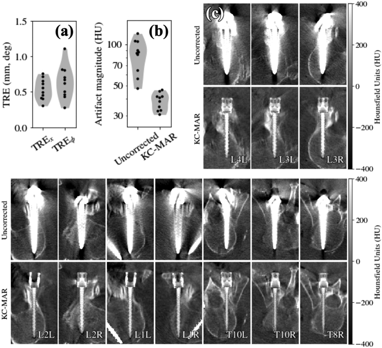
Cadaver study of KC-MAR imaging of pedicle screws. (a) Registration accuracy demonstrating ~0.5 mm and <1° TRE. (b) Artifact magnitude for uncorrected and KC-MAR images measured about the pedicle screws, showing 40%–80% reduction. (c) Uncorrected and KC-MAR images of 10 pedicle screws delivered to 6 vertebral levels; a tight grayscale window was chosen for visualization of nearby soft-tissue structures and to better illustrate pedicle breaches. Each image is a quasi-axial slice oriented to align with the long axis of a particular screw. Each image depicts two rendering techniques: the screw of interest in the quasi-axial slice is overlaid with a SIP rendering of the 3D component model; and other components that intersect the slice are rendered via simple voxel value replacement (>1000 HU). KC-MAR images show strong reduction in metal artifact and allow clearer visualization of the instrument and adjacent anatomy—e.g. placement of each screw within narrow pedicles.

In each case, quasi-axial slices are shown containing the long axis of the screw to clearly visualize placement of the screw within the pedicle corridor. Two rendering methods were used for the KC-MAR images in figure 5: (1) the in-plane screw is shown using a SIP rendering of the 3D screw model, giving a richer depiction of 3D screw morphology; and (2) the contralateral screw (which may partially intersect the slice) is shown simply using voxel replacement with a value >1000 HU for steel. In each case, the KC-MAR result gives markedly improved visualization of the screw (including threads) and polyaxial head relative to surrounding anatomy. In particular, note the improved visibility with respect to instances of mild lateral breach (L1R), mild anterior breach (T10R), and mild medial pedicle breach (T8R).

3.3. Cadaver study with spinal rods

The second cadaver study investigated KC-MAR performance in real anatomy using deformable component models representing curved stainless steel spinal rods. Results are summarized in figure 6. The convergence and accuracy of deformable registration are shown in figure 6(a), which plots the Hausdorff distance for the registered rod as a function of the number of B-spline control points in the deformable model. For the fairly realistic degree of curvature applied in these studies, a high degree of accuracy was achieved using 5 or 6 control points for a rod spanning 16 cm, yielding mean Hausdorff distance of 1.5 mm. Figure 6(b) shows axial slices for uncorrected (top) and KC-MAR (bottom) images for unilateral and bilateral rods. For the unilateral rods, KC-MAR exhibits nearly complete elimination of metal artifact. For the bilateral cases, the magnitude of artifact is much more severe, attributed to local projection data inconsistencies between views that are not resolved by the simple in-painting method used in the current work. While significantly reduced by KC-MAR (as quantified in figure 6(c)), residual artifacts are visible as faded bright streaks between the rods, corresponding to the view direction in which the rods are overlapping in projections. In the unilateral rod cases, artifact magnitude was reduced from 290 ± 98 HU to 69 ± 20 HU (76% reduction). Bilateral cases exhibited smaller gains in performance, reducing the artifacts to 90 ± 37 HU (66% reduction). Further reduction of these artifacts may be achieved with improved inpainting methods or a polyenergetic forward projection model that accounts for the material content of the known component and energy-dependent attenuation, which is the subject of future work as Discussed in section 4 below. Illustration of the reduction in artifacts for the steel rods is shown in figure 6(d) as maximum intensity projections (MIP), which highlight the reduction in blooming artifacts in close proximity to the rods.

Figure 6.

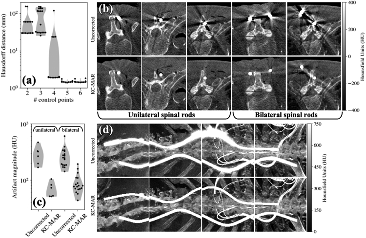
Cadaver study of KC-MAR imaging of deformable spinal rods. (a) Accuracy of deformable component registration plotted as a function of the number of spline control points. (b) Example axial slices for cases exhibiting unilateral and bilateral rods—Uncorrected (top) and KC-MAR (bottom). (c) Artifact magnitude without and with KC-MAR for unilateral and bilateral rods. (d) MIP renderings of CBCT reconstruction without correction (top) and with KC-MAR (bottom).

Finally, figure 7 shows images from the cadaver study involving both a polyaxial pedicle screw and a spinal rod, illustrating KC-MAR involving a combination of rigid and deformable components. The CBCT image without corrections in figure 7(a) demonstrates a severe level of artifact that could confound the ability to judge pedicle breach—in this case, for example, a possible medial breach. The KC-MAR result is rendered by voxel replacement in figure 7(b), showing improved visualization of the boundary of the screw shaft within the corridor (i.e. lack of medial breach). The 3D volume rendering of the known components in figure 7(c) further illustrates finer detail of the implant (e.g. threads) and visualization of the 3D spinal rod in relation to the attached screw and pertinent anatomy.

Figure 7.

KC-MAR using combined rigid (screw) and deformable (rod) registration at L4 vertebra, showing: (a) axial slice from a standard FBP reconstruction; (b) KC-MAR reconstruction with a conventional voxel replacement of the metal region; (c) 3D volume rendering of the known components with respect to the corrected image. (d) and (e) Overlay of the registered component model (screw cap and rod edges) on the uncorrected FBP image, demonstrating the accuracy of component registration in matching features down to the individual threads of the screw.

4. Discussion

An algorithm for MAR was presented that uses prior information of metal objects (referred to as ‘known components’) and 3D–2D registration to correct for metal artifacts in reconstructed images. The KC-MAR approach maintains the simplicity of conventional MAR, and the precise localization of metal components obtained by 3D–2D registration overcomes common pitfalls associated with 2D or 3D segmentation. The approach is compatible with more advanced sinogram completion strategies as well as methods based on component modeling discussed below. Compatibility with 3D FBP image reconstruction further supports suitability to intraoperative workflow, and the method is similarly suitable to MBIR methods that may further improve image quality and reduce dose.

KC-MAR was shown to reduce artifacts by 40%–80% and yield clear visualization of the anatomy close to the edge of the implant. Phantom studies served to establish algorithm parameters that were successfully translated to cadaver studies and allowed analysis of sensitivity to segmentation inaccuracies in a manner that was agnostic of any particular segmentation method. Dilation of the registered component by 1 pixel was observed to compensate for the residual artifacts, believed to be due to partial-volume effects, and offered additional robustness against potential errors in component modeling/manufacturing and geometric errors in reprojection.

Overestimation by larger than 1 pixel, however, resulted in interpolation artifacts and led to over-smoothing at the component boundary. Studies in a cadaver specimen using more complex components validated the algorithm under realistic clinical conditions. Rigid (screw) and deformable (rod) models in KC-MAR applied to CBCT images following implantation provided clear visualization of the surgical construct, including multiple components.

Residual artifacts following application of KC-MAR include streak artifacts attributed in part to slight misregistration or modeling/manufacturing errors of the component. Registration accuracy is affected by the spatial resolution in the projection data and could be improved, for example, by reading the detector at full-resolution, 1 × 1 pixel binning (see 2 × 4 binning required for the research system used in this work). An additional source of residual artifacts, such as the remaining faded streaks observed between bilateral rods, is likely associated with the particular technique for projection data processing—in this case, 2D interpolation within the component boundary. More advanced inpainting techniques will likely help to mitigate these residual artifacts, including methods that apply texture as well as intensity during interpolation (Bertalmio et al 2003) and more recent methods using deep learning for image- (Gjesteby et al 2017a) or sinogram-domain (Claus et al 2017) correction of regions containing metal. As an alternative to interpolation, the known material composition of components could also be used to correct for various spectral absorption and scatter effects. The approach by Meyer et al (2010a) involves estimation of scatter, where model mismatches were observed to result in residual artifacts similar to those observed above for bilateral rods (Star-Lack et al 2009). Beam-hardening correction as reported by Kyriakou et al (2010) offers a potential solution that relies only on the segmentation of the object without explicit modeling of physics. Alternatively (Xu et al 2017) modeled polyenergetic spectral effects of attenuation in metal, thereby better incorporating the available fluence (e.g. through the short axis of the screw) in the reconstruction process and better ensure local projection data consistency. For example, this could reduce the residual artifacts observed in the bilateral rod case, where the increased path length of the metal (due to overlapping rods in the projection domain) is ignored by simple inpainting.

The proposed algorithm by design requires prior knowledge on the metal components. In the case of a revision surgery with prior unidentified instrumentation, a generic parameterized screw model could be used to classify its diameter and length as in Uneri et al (2015). In cases where the component model is not known, the deformable formulation presented for the spinal rods could be extended to represent other types of instruments, for example by adopting more generalized spline models that apply to arbitrary surface (not just instruments with a cylindrical profile). For other cases in which modeling is not feasible, KC-MAR could also be used in conjunction with other algorithms that use projection-correction (Meyer et al 2010b), benefiting from improved accuracy when additional information is available. The runtime for the current implementation on single GPU (GeForce GTX TITAN, Nvidia, Santa Clara CA) was < 1 min for registration (and <2 min for FBP reconstruction). While the method shows promise, additional improvements would be necessary prior to integration within routine clinical workflow. One simple way to improve runtime would be to overlap data transfer (detector readout) with computation (registration, inpainting, and filtering). This would be possible since the registration step only requires a subset of the images—i.e. the initial 90° rotation of the orbit would provide the necessary data to run 3D–2D registration. Registration runtime would also improve with the accuracy of initialization in 3D–2D registration. A variety of recent advances, including machine learning techniques as in Esfandiari et al (2018), provide possible means of accurate initialization directly from the projection data, whereas the current work initialized the registration process according to the surgical plan. For example, a neural network trained according to KC models could be used to detect implants within the projection data and compute an accurate pose initialization.

References

- Anderla A, Culibrk D, Delso G and Mirkovic M 2013. MR image based approach for metal artifact reduction in x-ray CT Sci. World J. 2013 524243. [DOI] [PMC free article] [PubMed] [Google Scholar]
- Bal M and Spies L 2006. Metal artifact reduction in CT using tissue-class modeling and adaptive prefiltering Med. Phys. 33 2852–9 [DOI] [PubMed] [Google Scholar]
- Bal M, Celik H, Subramanyan K, Eck K and Spies L 2005. A radial adaptive filter for metal artifact reduction Proc. SPIE 5747 [Google Scholar]
- Barber CB, Dobkin DP and Huhdanpaa H 1996. The quickhull algorithm for convex hulls ACM Trans. Math. Softw 22 469–83 [Google Scholar]
- Bertalmio M, Vese L, Sapiro G and Osher S 2003. Simultaneous structure and texture image inpainting IEEE Trans. Image Process 12 882–9 [DOI] [PubMed] [Google Scholar]
- Boehm W 1980. Inserting new knots into B-spline curves Comput. Des 12 199–201 [Google Scholar]
- Brooks RA and Di Chiro G 1976. Beam hardening in x-ray reconstructive tomography Phys. Med. Biol 21 390–8 [DOI] [PubMed] [Google Scholar]
- Cho Y, Moseley DJ, Siewerdsen JH and Jaffray DA 2005. Accurate technique for complete geometric calibration of cone-beam computed tomography systems Med. Phys. 32 968. [DOI] [PubMed] [Google Scholar]
- Claus BEH, Jin Y, Gjesteby LA, Wang G and De Man B 2017. Metal-artifact reduction using deep-learning based sinogram completion: initial results 14th Int. Meeting on Fully Three-Dimensional Image Reconstruction in Radiology and Nuclear Medicine pp 631–5 [Google Scholar]
- De Man B, Nuyts J, Dupont P, Marchal G and Suetens P 2001. An iterative maximum-likelihood polychromatic algorithm for CT IEEE Trans. Med. Imaging 20 999–1008 [DOI] [PubMed] [Google Scholar]
- Esfandiari H, Newell R, Anglin C, Street J and Hodgson AJ 2018. A deep learning framework for segmentation and pose estimation of pedicle screw implants based on C-arm fluoroscopy Int. J. Comput. Assist. Radiol. Surg 13 1269–82 [DOI] [PubMed] [Google Scholar]
- Feldkamp LA, Davis LC and Kress JW 1984. Practical cone-beam algorithm J. Opt. Soc. Am A 1 612–9 [Google Scholar]
- Gjesteby L, Yang Q, Xi Y, Claus B, Jin Y, De Man B and Wang G 2017b. Reducing metal streak artifacts in CT images via deep learning: pilot results 14th Int. Meeting on Fully Three-Dimensional Image Reconstruction in Radiology and Nuclear Medicine pp 611–4 [Google Scholar]
- Gjesteby L, Yang Q, Xi Y, Claus B, Jin Y, De Man BEH, Wang G and Shan H 2017a. Deep learning methods for CT image-domain metal artifact reduction Proc. SPIE 10391 103910W [Google Scholar]
- Hansen N and Ostermeier A 2001. Completely derandomized self-adaptation in evolution strategies Evol. Comput. 9 159–95 [DOI] [PubMed] [Google Scholar]
- Hosntalab M, Aghaeizadeh Zoroofi R, Abbaspour Tehrani-Fard A and Shirani G 2008. Segmentation of teeth in CT volumetric dataset by panoramic projection and variational level set Int. J. Comput. Assist. Radiol. Surg 3 257–65 [Google Scholar]
- Hsieh J, Molthen RC, Dawson CA and Johnson RH 2000. An iterative approach to the beam hardening correction in cone beam CT Med. Phys. 27 23–9 [DOI] [PubMed] [Google Scholar]
- Idris AE and Fessler JA 2003. Segmentation-free statistical image reconstruction for polyenergetic x-ray computed tomography with experimental validation Phys. Med. Biol 48 2453–77 [DOI] [PubMed] [Google Scholar]
- Jin P, Bouman CA and Sauer KD 2015a. A model-based image reconstruction algorithm with simultaneous beam hardening correction for x-ray CT IEEE Trans. Comput. Imaging 1 200–16 [Google Scholar]
- Jin P, Ye DH and Bouman CA 2015b. Joint metal artifact reduction and segmentation of CT images using dictionary-based image prior and continuous-relaxed potts model IEEE Int. Conf. on Image Processing (ICIP) (Quebec City, QC, 27–30 September 2015) pp 798–802 [Google Scholar]
- Kalender WA, Hebel R and Ebersberger J 1987. Reduction of CT artifacts caused by metallic implants Radiology 164 576–7 [DOI] [PubMed] [Google Scholar]
- Karimi S, Cosman P, Wald C and Martz H 2012. Segmentation of artifacts and anatomy in CT metal artifact reduction Med. Phys. 39 5857–68 [DOI] [PubMed] [Google Scholar]
- Kataoka ML, Hochman MG, Rodriguez EK, Lin P-JP, Kubo S and Raptopolous VD 2010. A review of factors that affect artifact from metallic hardware on multi-row detector computed tomography Curr. Problems. Diagn. Radiol 39 125–36 [DOI] [PubMed] [Google Scholar]
- Klotz E, Kalender WA, Sokiransky R and Felsenberg D 1990. Algorithms for the reduction of CT artifacts caused by metallic implants Proc. SPIE 1234 [Google Scholar]
- Kuya K, Shinohara Y, Kato A, Sakamoto M, Kurosaki M and Ogawa T 2017. Reduction of metal artifacts due to dental hardware in computed tomography angiography: assessment of the utility of model-based iterative reconstruction Neuroradiology 59 231–5 [DOI] [PubMed] [Google Scholar]
- Kyriakou Y, Meyer E, Prell D and Kachelrieß M 2010. Empirical beam hardening correction (EBHC) for CT Med. Phys. 37 5179–87 [DOI] [PubMed] [Google Scholar]
- La Rivière PJ, Bian J and Vargas PA 2006. Penalized-likelihood sinogram restoration for computed tomography IEEE Trans. Med. Imaging 25 1022–36 [DOI] [PubMed] [Google Scholar]
- Lemmens C, Faul D and Nuyts J 2009. Suppression of metal artifacts in CT using a reconstruction procedure that combines MAP and projection completion IEEE Trans. Med. Imaging 28 250–60 [DOI] [PubMed] [Google Scholar]
- Meyer E, Maas C, Baer M, Raupach R, Schmidt B and Kachelries M 2010a. Empirical scatter correction (esc): a new CT scatter correction method and its application to metal artifact reduction IEEE Nuclear Science Symp. & Medical Imaging Conf. (Knoxville, TN, 30 October–6 November 2010) pp 2036–41 [Google Scholar]
- Meyer E, Raupach R, Lell M, Schmidt B and Kachelrieß RM 2012. Frequency split metal artifact reduction (FSMAR) in computed tomography Med. Phys. 39 1904–16 [DOI] [PubMed] [Google Scholar]
- Meyer E, Raupach R, Lell M, Schmidt B, Kachelriess M and Kachelrieß M 2010b. Normalized metal artifact reduction (NMAR) in computed tomography Med. Phys. 37 5482–93 [DOI] [PubMed] [Google Scholar]
- Morin RL and Raeside DE 1981. A pattern recognition method for the removal of streaking artifact in computed tomography Radiology 141 229–33 [DOI] [PubMed] [Google Scholar]
- Moseley DJ, Siewerdsen JH and Jaffray DA 2005. High-contrast object localization and removal in cone-beam CT Proc. SPIE 5745 [Google Scholar]
- Mouton A, Flitton GT, Bizot S, Megherbi N and Breckon TP 2013. An evaluation of image denoising techniques applied to CT baggage screening imagery 2013 IEEE Int. Conf. on Industrial Technology (ICIT) (Cape Town, South Africa, 25–28 February 2013) pp 1063–8 [Google Scholar]
- Pauwels R, Jacobs R, Bosmans H, Pittayapat P, Kosalagood P, Silkosessak O and Panmekiate S 2014. Automated implant segmentation in cone-beam CT using edge detection and particle counting Int. J. Comput. Assist. Radiol. Surg 9 733–43 [DOI] [PubMed] [Google Scholar]
- Penney GP, Weese J, Little JA, Desmedt P, Hill DL and Hawkes DJ 1998. A comparison of similarity measures for use in 2D-3D medical image registration IEEE Trans. Med. Imaging 17 586–95 [DOI] [PubMed] [Google Scholar]
- Rinkel J, Dillon WP, Funk T, Gould R and Prevrhal S 2008. Computed tomographic metal artifact reduction for the detection and quantitation of small features near large metallic implants J. Comput. Assist. Tomogr 32 621–9 [DOI] [PubMed] [Google Scholar]
- Ruth V, Kolditz D, Steiding C and Kalender WA 2017. Metal artifact reduction in x-ray computed tomography using computer-aided design data of implants as prior information Invest. Radiol. 52 349–59 [DOI] [PubMed] [Google Scholar]
- Star-Lack J, Sun M, Kaestner A, Hassanein R, Virshup G, Berkus T and Oelhafen M 2009. Efficient scatter correction using asymmetric kernels Proc. SPIE 7258 72581Z [Google Scholar]
- Stayman JW, Otake Y, Prince JL, Khanna AJ and Siewerdsen JH 2012. Model-based tomographic reconstruction of objects containing known components IEEE Trans. Med. Imaging 31 1837–48 [DOI] [PMC free article] [PubMed] [Google Scholar]
- Uneri A et al. 2016. Deformable 3D-2D registration of known components for image guidance in spine surgery Med. Image Comput. Comput. Assist. Interv 9902 124–32 [DOI] [PMC free article] [PubMed] [Google Scholar]
- Uneri A et al. 2017. Intraoperative evaluation of device placement in spine surgery using known-component 3D-2D image registration Phys. Med. Biol 62 3330–51 [DOI] [PMC free article] [PubMed] [Google Scholar]
- Uneri A, De Silva T, Stayman JW, Kleinszig G, Vogt S, Khanna AJ, Gokaslan ZL, Wolinsky J-P and Siewerdsen JH 2015. Known-component 3D-2D registration for quality assurance of spine surgery pedicle screw placement Phys. Med. Biol 60 8007–24 [DOI] [PMC free article] [PubMed] [Google Scholar]
- Uneri A, Yi T, Zhang X, Stayman J, Helm P, Osgood G, Theodore N and Siewerdsen J 2018a. 3D-2D known-component registration for metal artifact reduction in cone-beam CT Int. Conf. Image Formation in X-Ray Computed Tomography pp 151–5 [Google Scholar]
- Uneri A, Zhang X, Yi T, Stayman JW, Helm PA, Theodore N and Siewerdsen JH 2018b. Image quality and dose characteristics for an O-arm intraoperative imaging system with model-based image reconstruction Med. Phys. 45 4857–68 [DOI] [PMC free article] [PubMed] [Google Scholar]
- Wei J, Chen L, Sandison GA, Liang Y and Xu LX 2004. X-ray CT high-density artefact suppression in the presence of bones Phys. Med. Biol 49 5407–18 [DOI] [PubMed] [Google Scholar]
- Xu S, Uneri A, Khanna AJ, Siewerdsen JH and Stayman JW 2017. Polyenergetic known-component CT reconstruction with unknown material compositions and unknown x-ray spectra Phys. Med. Biol 62 3352–74 [DOI] [PMC free article] [PubMed] [Google Scholar]
- Yazdia M, Gingras L and Beaulieu L 2005. An adaptive approach to metal artifact reduction in helical computed tomography for radiation therapy treatment planning: experimental and clinical studies Int. J. Radiat. Oncol 62 1224–31 [DOI] [PubMed] [Google Scholar]
- Yu H, Zeng K, Bharkhada DK, Wang G, Madsen MT, Saba O, Policeni B, Howard MA and Smoker WRK 2007. A segmentation-based method for metal artifact reduction Acad. Radiol. 14 495–504 [DOI] [PMC free article] [PubMed] [Google Scholar]
- Zatz LM and Alvarez RE 1977. An inaccuracy in computed tomography: the energy dependence of CT values Radiology 124 91–7 [DOI] [PubMed] [Google Scholar]
- Zhang X, Uneri A, Stayman JW, Zygourakis CC, Lo S f L, Theodore N and Siewerdsen JH 2019. Known-component 3D image reconstruction for improved intraoperative imaging in spine surgery: a clinical pilot study Med. Phys. ( 10.1002/mp.13652) [DOI] [PMC free article] [PubMed] [Google Scholar]
- Zhang Y and Yu H 2018. Convolutional neural network based metal artifact reduction in x-ray computed tomography IEEE Trans. Med. Imaging 37 1370–81 [DOI] [PMC free article] [PubMed] [Google Scholar]
- Zhang Y, Zhang L, Zhu XR, Lee AK, Chambers M and Dong L 2007. Reducing metal artifacts in cone-beam CT images by preprocessing projection data Int. J. Radiat. Oncol 67 924–32 [DOI] [PubMed] [Google Scholar]