Preprocessing Breast Cancer Data to Improve the Data Quality, Diagnosis Procedure, and Medical Care Services

Abstract

In recent years, due to an increase in the incidence of different cancers, various data sources are available in this field. Consequently, many researchers have become interested in the discovery of useful knowledge from available data to assist faster decision-making by doctors and reduce the negative consequences of such diseases. Data mining includes a set of useful techniques in the discovery of knowledge from the data: detecting hidden patterns and finding unknown relations. However, these techniques face several challenges with real-world data. Particularly, dealing with inconsistencies, errors, noise, and missing values requires appropriate preprocessing and data preparation procedures. In this article, we investigate the impact of preprocessing to provide high-quality data for classification techniques. A wide range of preprocessing and data preparation methods are studied, and a set of preprocessing steps was leveraged to obtain appropriate classification results. The preprocessing is done on a real-world breast cancer dataset of the Reza Radiation Oncology Center in Mashhad with various features and a great percentage of null values, and the results are reported in this article. To evaluate the impact of the preprocessing steps on the results of classification algorithms, this case study was divided into the following 3 experiments:

Breast cancer recurrence prediction without data preprocessing

Breast cancer recurrence prediction by error removal

Breast cancer recurrence prediction by error removal and filling null values

Then, in each experiment, dimensionality reduction techniques are used to select a suitable subset of features for the problem at hand. Breast cancer recurrence prediction models are constructed using the 3 widely used classification algorithms, namely, naïve Bayes, k-nearest neighbor, and sequential minimal optimization. The evaluation of the experiments is done in terms of accuracy, sensitivity, F-measure, precision, and G-mean measures. Our results show that recurrence prediction is significantly improved after data preprocessing, especially in terms of sensitivity, F-measure, precision, and G-mean measures.

Introduction

Cancer is 1 of the causes of mortality in different human societies. The incident rate of various types of cancer differs among different regions and ethnicities. Breast cancer is among common cancers in women from different countries, on which a great deal of research has been conducted. On the other hand, breast cancer can recur after each treatment. Usually, recurrence occurs within 3 to 5 years after the treatment, locally, regionally, or distant metastasis.¹ Prediction of recurrence is important because it decreases the chance of recovery.

The epidemiological pattern of breast cancer in Iran is similar to that of other Eastern Mediterranean and developing countries. The mean age of patients with breast cancer in Iran is between 40 and 50 years and is 10 and 15 years lower than that in the developed countries and the global mean age.² According to Breast Cancer Statistics,³ 268 670 new breast cancer cases and 41 400 breast cancer deaths have occurred in the United States in 2018. Moreover, according to the information obtained from the World Health Organization (in the years 2012 and 2013), breast cancer is 1 of the most severe diseases in women in developed and developing countries. Approximately, 1.3 million women suffer from breast cancer annually; some of whom die due to the unavailability of timely treatment. In the United States, breast cancer is the most prevalent cancer among women and the second cause of cancer mortality. In Taiwan, according to the Statistics Report of Bureau of Health Promotion, Department of Health (2012), there were more than 9000 women affected by breast cancer and 1800 women had died from it. Also, breast cancer has been the most common cancer in women and has been the fourth cause of cancer mortality in Taiwan. Cancer statistics show that breast cancer is considered 1 of the most serious threats to women’s health.^4,5 According to a World Health Organization report, 80 of 1000 women are affected by this type of cancer every year, most of whom live in Third-World countries.⁶

Given the importance of this issue, over the years, many studies have been conducted on issues such as calculating survival time, accuracy in diagnosis, and recurrence rate of breast cancer,^1,7-12 most of which have used public datasets (such as The surveillance, epidemiology and end results [SEER], Wisconsin), whose values have been simulated or have been belonged to a particular country’s population. Such data have problems such as the following:

1. Proposed models on benchmark datasets are not suitable for practical uses of other existing datasets and do not have the necessary efficiency.

2. In studying cancer, there is a wide variety of features, some of which may exist between different datasets. For example, among the datasets of the Reza Radiation Oncology Center (RROC), there are features that have not been considered in any of the benchmark datasets.

3. The preprocessed benchmark datasets are usually abstract, and the obtained results of research done on them cannot be used in practice.

4. Some available datasets contain no (or a small percentage of) missing data. This assumption is not true in real medical data. Therefore, the method of handling this issue is different among different datasets.

5. The results obtained from benchmark datasets cannot be generalized to countries with different populations, as each country has a unique climate, food, and culture.

Considering what mentioned above, the availability of a real-world dataset containing information related to the country’s characteristics can help in the discovery and identification of its realities.

However, it should also be noted that most real-world data face important challenges such as low data quality (existence of errors, inconsistency, noise, missing values, etc). Therefore, if data mining is performed on poor-quality data, even using the most powerful and optimal algorithms, the obtained results can be inaccurate and unreliable. Thus, the application of preprocessing on the data (to improve data quality) before the data mining process is indispensable.

On the other hand, data preprocessing is a step in the process of knowledge discovery that takes about 60% to 90% of the time needed for knowledge discovery and accounts for 75% to 90% of the success of data mining projects. Therefore, in the case of no or poor data preprocessing, the data mining process will fail.¹³

In this regard, several studies have been performed on data preprocessing of medical datasets.^14-19 In Peng et al²⁰ for classification of high dimensionality medical data, a new feature selection method has been presented. The paper aimed at improving the performance of classifiers based on the selected features. The results showed that the proposed feature selection method had been better than the sequential forward floating search method and had led to the better performance of the classifiers.

In Majid et al,²¹ a method has been proposed for predicting breast and colon cancers in an unbalanced dataset. First, to balance the dataset, the samples of the minority class have been increased by oversampling, and then, prediction models have been used.

In the research conducted by Pedro et al, a 5-year survival prediction of patients with breast cancer has been done on the real data of Portuguese Cancer Institute. That dataset contains a high percentage of missing data. The authors aimed to study the effect of missing value assignment on survival model prediction. The results showed that the k-nearest neighbor (k-NN) algorithm yielded the best results among other prediction models.²²

Considering the literature review, most of the papers have been focused on a single preprocessing technique, such as dimensionality reduction, alleviating the imbalanced data problem, filling in the missing values, etc. In this study, we investigate a wide range of techniques, and then, a set of appropriate preprocessing methods has been selected considering the nature of data with the aim of improving the classification performance. Consequently, this article has the potential to be considered as a guide to applying the appropriate preprocessing methods on real-world data.

In this article, some preprocessing methods, such as error correction, resolving data inconsistency, noise removal, filling null values, and feature selection have been applied to the RROC breast cancer dataset. Considering that at first, only 40% of feature values of the RROC dataset had been filled, this study aimed to examine the effect of preprocessing on improving the data quality, as well as the results of the classification algorithms.

The rest of the article is organized as follows. In section “Materials and the Dataset,” the RROC dataset is introduced and the preprocessing methods have been described. Section “Decision Methods” explains the decision methods and evaluation measures. In section “Results and Discussion,” the results of the experiments have been reported, discussed, and compared with previous studies. Finally, the conclusion has been provided in section “Conclusion and Future Studies.”

It is needed to mention that the terms feature and attribute are used in this text interchangeably. Also, the terms record and sample are used instead.

Materials and the Dataset

In this section, the dataset, the process of improving the data for the prediction models, and the steps in the case study have been defined.

The RROC breast cancer dataset

The RROC dataset has been collected cross-sectionally from 2009 to 2014 using the records of patients with malignant breast cancer of the RROC in Iran, Mashhad, and has been entered manually into SPSS software. This dataset contained 1923 records with 101 features, some of which have been described in Table 1. To predict the recurrence of cancer, the recurrence feature was considered a class attribute containing the values of recurrences and no recurrences. Therefore, the problem at hand is a 2-class problem in which positive label means cancer recurrence and negative class is nonrecurrence.

Table 1.

Reza Radiation Oncology Center breast cancer data description of attributes.

Explanation	Attribute name
Patient’s age	Age
Age at marriage	marriage
Number of gravidity	g
Number of pregnancy	p
Number of dead births	d
Number of alive births	al
Number of abortions	ab
TNM classification of the tumor{t1, t2, t3, t4}	t-tnm
TNM classification of the lymph node{n0, n1, n2, n3}	n-tnm
TNM classification of the metastasis{m0, m1}	m-tnm
Number of lymph nodes involved	node involve
Type of surgery operation{MRM, BSC}	surgery
Has the patient had a history of cancer in the family? {yes, no}	familyh
Family relationship with someone who has cancer {mother, father, etc}	relation
Sort of cancer in relatives of patients{breast, lung, etc}	sort
Was radiotherapy applied to the patient?{yes, no}	Rt
Radiation dose rate	dose
Was adjuvant chemotherapy applied to the patient?{yes, no}	Chemotherapy
Was neoadjuvant chemotherapy applied to the patient?{yes, no}	Neo
Was hormone therapy applied to the patient or is not{yes, no}	Hormone1
Estrogen receptor state{negative, positive}	er
Progesterone receptor state{negative, positive}	pr
The latest condition of the patient	lastcon
Has the patient’s cancer recurred?{yes, no}	recc

Abbreviations: MRM, modified radical mastectomy; TNM, tumour, node, metastasis; BSC, breast-conserving surgery.

In the recurrence attribute, 1820 of 1923 records were labeled, from which only 78 records contained recurrences and 1742 records contained no recurrence values.

Presenting a general plan to improve data quality for prediction models

1. Introduction to the concept of each field in the dataset (meaning, domain type, value range, and the acceptable values for each field)

2. Identifying the inter-relations between fields (conceptual relations and dependencies)

3. Taking a statistical summary of the dataset (mean, maximum, minimum, drawing histogram for each field, etc)

4. Identifying the possible errors in the dataset, identifying the missing and null values

5. Choosing the appropriate preprocessing based on the nature of the dataset

   • Error correction (noise, inconsistency, outliers, out-of-range values)

   • Filling missing and null values

   • Dealing with the unbalanced datasets.

   • Data reduction (feature subset selection, compression, etc)

6. Constructing prediction models before data preprocessing and after applying each preprocessing method

7. Analyzing prediction results before and after data preprocessing and examining the extent of data quality improvement after applying the appropriate preprocessing models

A case study of data preprocessing in the RROC dataset

In the first step, the CRISP data mining methodology (cross-industry standard process for data mining)²³ was taken as a guide to the case study. Then, a brief acquaintance with the concepts of cancer, including breast cancer and the related issues, was made. Considering that unlike benchmark datasets, the real-world datasets often have no documentation of feature concepts; to get a correct understanding of the data, the concepts and domain of each feature were identified with the help of the authentic sources and the experts’ opinions in the field of cancer, and the interpretation booklet of the dataset was documented.

In the next step, because the dataset problems were unknown, a statistical summary of the features should be prepared using SPSS software before starting the process of analyzing the data, so that the nature of the dataset was known. In the statistical summary, mean, mode, median, standard deviation, minimum, and maximum were used for numeric attributes, and frequency tables and histogram drawing were used for nominal attributes. Moreover, the number of existing and missing values for each attribute was determined. The results suggested that some of the attributes had outliers, noise, out-of-range values, and missing values. In this step, even some of the patterns were identified (for example, a pattern like the existence of masses in the left breast of most Iranian women).

After a brief acquaintance with the dataset, the data analysis was performed in the 3 steps of the case study. In what follows, the case study is described according to Figure 1, consisting of

Figure 1.

The steps of case study in RROC.

RBF indicates radial basis function; RROC, Reza Radiation Oncology Center; SMO, sequential minimal optimization.

1. predicting breast cancer recurrence without data preprocessing

2. predicting breast cancer recurrence after preprocessing

3. predicting breast cancer recurrence by filling null values.

Recurrence prediction without preprocessing

In this step, the data quality was examined. Data quality was determined based on the purpose of using the data, consisting of the factors such as accuracy, completeness, consistency, believability, and interpretability.²⁴ The accuracy, completeness, and consistency have a greater importance in medical datasets as errors are integral to most of them, and in the case of extracting knowledge with poor-quality data, the results obtained face a low confidence level and are sometimes inaccurate. Therefore, to investigate the quality of the dataset, first, a number of basic classification algorithms, ensemble methods, and feature subsets were chosen. Some of the feature subsets were chosen using Weka software, and some others were chosen based on the domain knowledge and papers related to the breast cancer. Then, recurrence prediction models were constructed on different feature subsets. After analyzing the algorithm results, the prediction of the AdaBoost algorithm on 1 of the feature subsets was unexpectedly excellent (69 of 78 recurrence records and all 1742 no recurrence records were predicted accurately). The obtained result looked unusual regarding the existence of errors, noise, inconsistencies, and null values, etc, in the dataset. Thus, after some analyses (described in section “Results and Discussion”), it became obvious that the excellent prediction of this algorithm was due to the existence of a result attribute in that feature subset.

Result attribute is an attribute for which if the prediction models are constructed on it, they will predict well that attribute, regardless of the other attributes. Therefore, the prediction models were reconstructed after the recurrence date attribute was removed from all feature subsets; but then none of the algorithms predicted well any longer. The main reason was the low quality of the dataset. Therefore, applying data preprocessing before analyzing the data is essential to have a successful data mining process. Hence, in the later steps, appropriate data preprocessing methods were chosen and applied based on the nature of the dataset. Moreover, given that some classification algorithms are the modifications or improvements of other methods and regarding the aim of this article, from among different classification algorithms, 3 basic algorithms of naïve Bayes, k-NN, and sequential minimal optimization (SMO) were chosen. One of the reasons for selecting these algorithms was their simplicity, as the use of complex algorithms would increase the probability of errors and would make analyzing their results more difficult. Also, the way these algorithms work are neither too different nor too similar to each other to make their results comparable. Therefore, finally, the 3 above-mentioned algorithms were chosen.

Recurrence prediction after preprocessing

In this step, data quality was examined for accuracy and consistency. There was a possibility of error in data registration because of human involvement. Data registrars extracted the needed data through the study of the medical records of the patients, pathological reports, radiotherapy and chemotherapy files, etc, and entered them electronically. Moreover, the patients might not be in appropriate conditions and might not remember some information such as the date related to the first pregnancy, weight, etc, or might not be willing to fill in some information such as addiction, divorce status, etc. Thus, the patients might fill some information by mistake or leave them unfilled. Therefore, errors are integral to medical data. In case of existence of errors in the data, the prediction might be done wrongly and the lives of the patient might be endangered. Thus, to improve the data quality, errors in the RROC dataset were identified in the first step of preprocessing by scrutinizing the registered fields and identifying the available inconsistencies in them. The errors were placed in the following categories:

1. Out_of_value_range errors

2. Calculation errors

3. Logical errors

4. Inconsistency errors

5. Medical standard errors

6. Conceptual errors.

As an example, in the RROC dataset, 1 stood for female and 2 for male in the field of sex, so the appearance of any value other than 1 and 2 signified an out_of_value_range error. Or in the field of age of first pregnancy whose value ranged from 13 to 40 years, a value of 5 indicated an out_of_value_range error. Some errors were identifiable through algebraic relations. For example, the number of abortions was determined by subtraction of the fields’ number of gravidity and pregnancy. Thus, if in a record the subtraction of the fields’ number of gravidity and pregnancy differed from the number of abortions, a calculation error had been occurred. Or as another example, the sum of live births and stillbirths determined the number of pregnancies, and the inconsistent values signified a calculation error. On the other hand, some errors seemed logically wrong, for example, when the patient weight had been entered 12 or the abortion age had been entered 5. If in a record the age of first pregnancy had a value but the number of pregnancies had been entered 0, inconsistency had been occurred. Also, in the field of cancer, the amount of radiotherapy doses received by a patient followed a specific standard, and in case it was out of the range of the standard defined in the medicine, a medical standard error had been occurred. The last type of errors was conceptual errors, which were identified with respect to the concepts of each field. For example, in the case of breast cancer, the period of receiving radiotherapy was between 5 and 6 months, and if the difference between the start and end date of radiotherapy was more than 5 to 6 months, a conceptual error has been occurred. Therefore, if the researcher did not have a good understanding of the concept of breast cancer radiotherapy period, she or he would not notice the existence of error in data by the appearance of the start and end date of radiotherapy.

On the other hand, to identify errors in the dataset, it should also be noted that some errors were complex, meaning that they could not be identified by merely looking at 1 field, and the values in several fields of a record needed to be looked at. As an example, if the field of sex in a record contained male and the number of pregnancies contained the value of 2, an error had been occurred, whereas if the value of each of these fields was considered alone, no error would be identified because the value of each of the aforementioned fields was in the range of their acceptable values. As a result, in this research, the errors in each field and each record were identified separately through discovering the rules and relations based on features of the dataset. In the next section, the identification methods of errors have been stated separately.

The method of identifying possible errors in each field

To identify the possible errors in each field, first, the data type, the domain, the acceptable values, the value range, and the value format of each attribute were identified separately. For example, for the weight attribute, its type was numerical, its domain was real numbers, the acceptable values were from 37 to 120, the value range was between 45 and 100, and its format was decimal. Then, with respect to what mentioned above, if the values of any field were out of their properties, errors had been occurred. For instance, if the value of 11.5 had been entered for the weight attribute, an error had been occurred because the acceptable value for the weight attribute was between 37 and 120 and, therefore, 11.5 was noise. Also, if the value of 37 was entered for weight, the data were outlier because the value range was between 45 and 100. Moreover, entering the value of “H” for the weight attribute was error because the attribute type was numerical and “H” was categorical. Thus, the errors were identified and resolved by using the information obtained from the characteristics of each field.

The method of identifying possible errors in each record

To detect the possible errors in each record, discovering the rules based on other features was needed. Thus, the conceptual relationships and interdependencies between attributes had to be identified. To do this, an accurate understanding of the concepts of each attribute was first achieved. Then, the attributes that were conceptually similar to each other and the attributes whose values were dependent on each other’s values were identified and their inter-relations were discovered using the expert opinion or the domain knowledge. For example, in the RROC dataset, the attributes of n and the lymph nodes involved were examples of attributes that were conceptually close to each other. After the identification of these 2 fields, their inter-relations were determined using the expert opinion. Physicians determined the value of n from the number of lymph nodes involved. In error detection of the RROC dataset, this conceptual relation was 1 of the relations used in the error detection. For example, if the number of lymph nodes involved was between 1 and 3 and the value of n was not equal to 1, a conceptual error had been occurred because the values of n were in the range of 0 to 3, considering the number of lymph nodes involved. Furthermore, in the RROC dataset, the attributes of marital status, age at marriage, and the number of children were the example of the attributes dependent on each other. For example, if in a record the patient was single but the fields of age at marriage and number of children had values, errors had been occurred. Therefore, by the identification of the dependent attributes and by checking their values in each record, errors could be identified.

Regarding what mentioned above, the errors in the RROC dataset with 194 223 fields (ie, 101 × 1923 fields × records) were identified and documented based on the characteristics of each field as well as the discovered inter-relations and interdependencies between features. Then, the error documents were reported to the data registration center, and this center corrected or removed some error values, or added new values to the missing fields. Overall, 999 fields were improved in this part. Also, these changes were applied for 72 attributes and 670 records.

Next, some of the errors were resolved with through the standards obtained from the domain knowledge, like the relation between the 2 fields of lymph nodes involved and n, or were replaced and modified using the most likely value in a given attribute. For example, if the number of lymph nodes involved was between 4 and 9, the correct value of n would be 2. If n was not 2, its value would be replaced by 2 to resolve the error. In 2.26% of the records of the RROC dataset, the value assignment of n based on the number of the lymph nodes involved was contrary to the medical standard. Thus, in 97.74% of the cases, the values of n had been categorized correctly, given the number of lymph nodes involved in the cancer. Therefore, at the time of error, the probability of n being entered incorrectly was much higher than the number of the lymph nodes involved. Also, if the patient was single but the fields of age at marriage, number of live births, stillbirth, abortion age, and number of abortions had values, the value of single changed to married because there was less likelihood that all the fields of age at marriage, number of live births, etc, were entered incorrectly and the value of single was entered correctly. As the attribute values of marital status for most patients was married, there was a higher probability that the value of single was incorrectly entered instead of married. After correcting such errors, 494 more fields were also improved. Thus, 1493 fields were changed after error corrections. Therefore, before constructing the prediction models, irrelevant and redundant attributes should be identified and removed.

The relevancy of the attributes depends on the classification aim, which is the recurrence prediction in the problem at hand. For example, in the RROC dataset, attributes such as pathology laboratory name, pathology laboratory code, and academic degree are irrelevant. Also, before constructing the prediction models, redundant attributes should be identified and removed based on the correlation of the features. Examples of the removed redundant features from the RROC dataset are live births and tumour, node, metastasis (TNM). As the live birth attribute could be determined based on the number of gravidity and pregnancy, number of abortions, and number of stillbirths, its presence in the dataset is superfluous. Also, the values t, n, and m were retrievable from the attribute TNM, making this attribute removable.

After removing irrelevant and redundant attributes, feature selection was performed on the remaining attributes. Finally, prediction models were constructed on the modified dataset using different feature subsets.

Recurrence prediction by filling null values

In this step, in addition to the corrections applied for the dataset in the previous step, null values and missing values were filled according to the discovered patterns based on features.

Before explaining the process done in this step, the difference between null and missing values is described. In some cases, the lack of data does not mean missing data or error in data.²⁴ For example, in the RROC dataset, an individual might not have family history of cancer, so the field of cancer in family members would remain empty, which did not mean missing data, but it was due to having no content in this field. As a result, such values were called null values and the attributes whose contents were unknown were called missing values. Of course, it is necessary to note that if a questionnaire is designed correctly from the beginning of study, fewer null and missing values will be created. Nevertheless, facing such problems with real data is natural.

In this step, using the conceptual relations and dependencies discovered in the previous step, some patterns were defined. Then, with the help of these patterns, null values and missing values replaced with appropriate values. For examples of missing values, in the RROC dataset, 2 fields of tumor size and t are conceptually related. Oncologists calculate t value using the tumor size (with the help of medical standards). Considering this relationship, missing values of t can be filled according to the tumor size. As an example of null values, consider the dependency between the attributes of metastasis,ⁱ date of metastasis, and metastasis site. In the case that the patient did not have metastasis, the date field of metastasis and metastasis site were identified as null values and were filled by appropriate values in terms of type and domain of each field.

In the RROC dataset, after identifying the conceptual relations and dependencies between features, 31 patterns were discovered based on other features and each of the null and missing values was filled by appropriate values. For example, when the value of the addiction feature was no, it meant that the patient was not addicted. Thus, the lack of data in the fields of addiction type and addiction duration was indicative of null values. After identifying these 2 fields, their values were filled with no and 0, respectively, meaning that the patient consumed no narcotics and that his consuming duration was 0, too. Also for a missing value, when the receptors of progesterone and estrogen had a negative value, it meant that these receptors were not observed in the patient blood. Therefore, in case these attributes were negative, their percentages were assigned the value of 0.

Finally, after filling null and missing values in the RROC dataset, 32 506 fields received values, and practically 64 features and 1919 records were improved. Then, prediction models were constructed on the modified dataset using different feature subsets.

As previously stated, before the preprocessing, only 40% of the attributes of the original dataset contained values, but after the preprocessing methods were performed in the second and third steps, 78% of the final dataset contained values.

Decision Methods

In this section, the classification algorithms, feature selection methods, and the confusion matrix (CM) are described. The overall procedure is depicted in Figure 2.

Figure 2.

The overall procedure of the decision methods.

SMO indicates sequential minimal optimization.

Classification algorithms

Three classification algorithms are used in this research, namely, naïve Bayes, k-NN, and SMO classifier. We have employed the Weka as a widely used implementation of these algorithms. As mentioned in Kerdegari et al,²⁵ Weka is java-based data mining software. Weka contain a set of machine learning algorithms for data mining tasks such as preprocessing, classification, and feature selection. The graphical interface of Weka is called Explorer, and all the provided facilities can be accessed by means of this user interface.

Naïve Bayes classifier

This algorithm is derived from Bayes classifier which is robust in separating noise points and irrelevant attributes.^2,3 In addition, prediction models are constructed by this algorithm quickly.^4,5,26 Consider database D with n attributes (a₁, a₂, . . ., a_n) and m class labels (c₁, c₂, . . ., c_m). The sample x with the form x = (a₁, a₂, . . ., a_n) belongs to the class c_i if it has the highest conditional probability (Formula 1)

$$P\left(C_i|X\right)>P\left(C_k|X\right)k=1\mathrm{to}m\mathrm{and}k!=i$$ (1)

The probabilities, P(Ci|X), are calculated using the Bayes’ theorem according to Formula 2

$$P\left(C_i|X\right)=P\left(X/C_i\right)P\left(C_i\right)/P\left(X\right)$$ (2)

As the denominator of Formula 2 is equal for all the terms, it only remains for us to maximize the numerator. P(C_i) is calculated as follows

$$P\left(C_i\right)=\frac{S_i}{S}$$ (3)

where S_i is the number of samples related to the class i and S is the number of all samples/records.

To reduce the computational complexity, P(X|C) is calculated as follows

$$P\left(X|C_i\right)={\mathrm{\Pi }}_{k=1\dots n}P\left(X_k|C_i\right)$$ (4)

where X_k is the value of attribute a_k for record X.

If a_k is deterministic, P(X_k|C_i) is calculated as

$$P\left(X_k|C_i\right)=\frac{S_{ik}}{S}$$ (5)

where S_ik is the number of records labeled by class i whose values equal to X_k and S_i is the number of records labeled by class i. If a_k is continuous, the probability is computed using the Gaussian distribution.

IBK classifier

This classifier is the Weka implementation of the k-NN algorithm. k-nearest neighbor is a lazy and instance-based learner. The Instance-Based-K-neighbors (IBK) classifier is applicable for data with high variance distribution.⁵ As mentioned in Sirageldin et al,²⁷ to predict the label of a test sample by means of nearest neighbor rule, first of all, the distance between the test sample and all the training samples should be calculated using a distance measure such as the Euclidean distance. Then, k nearest training samples should be selected and the most common label of these samples should be considered as the label of the test sample.

Sequential minimal optimization classifier

This is an implementation of support vector machines (SVMs) in Weka.^25,28 Support vector machine classifier is a supervised learner. To classify the data, SVM uses a hyperplane as the model. The idea is to separate the data into 2 distinct categories with a large margin decision boundary. The training samples belong to 1 of the 2 categories. The SVM predicts the class of an instance based on the side of the hyperplane that the instance is placed. The SMO algorithm is used for training the SVM classifier using the polynomial or Gaussian kernel. In SMO, all the attributes are normalized by default and class attributes are converted to binary ones.

Feature selection

We have used 2 search methods to find the most suitable subset of the features: Genetic algorithm²⁹ and Ranker search.³⁰ The search methods need a measure to evaluate the appropriateness of a subset. Two evaluation measures were used in this study: Correlation-based and Gain Ratio Feature Evaluation measures. Therefore, we have 4 feature selection mechanisms combining the search methods and the evaluation measures.

Correlation-based feature evaluation measure is named cfsSubsetEval in the Weka. The idea of this method is to select those features that have high correlation with the class labels. On the other hand, the selected features should have least amount of correlation with each other.³¹

Gain Ratio Feature Evaluation measures is named GainRatioAttributeEval in Weka.³² The gain ratio calculates the information gain of a feature based on the entropy formula.

Performance evaluation

As mentioned in Section “Materials and the Dataset,” in this research, we have 2 classes, positive (ie, cancer recurrence) and negative (nonrecurrence). The performance of a classification algorithm can be represented by a 2 × 2 matrix denoted as CM. Each element CM_i,j of this matrix represents the number of test samples of class i predicted as class j. Evaluation measures are calculated regarding the CM of Table 2.

Table 2.

Confusion matrix for a 2-class problem.

		Predicted class
		Class = recurred	Class = non-recurred
Actual class	Class = recurred	True positive(TP)	False negative(FN)
	Class = nonrecurred	False positive(FP)	True negative(TN)

TP: The number of samples labeled as recurrence by the physician and correctly predicted by the classification algorithm as recurrence.

FN: The number of samples labeled as recurrence by the physician but wrongly predicted by the classification algorithm as no recurrence.

FP: The number of samples labeled as no recurrence by the physician but wrongly predicted by the classification algorithm as recurrence.

TN: The number of samples labeled as no recurrence by the physician and correctly predicted by the classification algorithm as no recurrence.

To compare the results of the classification algorithms, evaluation metrics are used. In this article, we use 5 measures, namely, accuracy, sensitivity, precision, F-measure, and G-means, to evaluate the performance of the classification algorithms.

The overall accuracy

It is determined by this measure that what percentage of all samples or what number of all samples are classified correctly. This is 1 of the most widely used classification evaluation measures which can be seen in Formula 6^10,33

$$Overallaccuracy=\frac{\left(TN+TP\right)}{\left(TP+FP+TN+FN\right)}$$ (6)

The accuracy measure assumes that the different values of a class have the same weight, although the data can be unbalanced. Therefore, for unbalanced data, it is best to use measures of sensitivity, precision, F-measure, and G-mean, in addition to the accuracy measure. For example, in the RROC dataset, the number of patients with recurrence was 78 and the number of patients without recurrence was 1742, represented. Then, if only 5 recurred and 1740 nonrecurred samples had been predicted correctly after the prediction, the accuracy measure was 96%, while the samples of the minority class would not be predicted well.

True positive rate

Formula 7 shows the extent to which a classifier can predict the samples of the positive class, ie, the recurred samples, correctly. True positive rate is a measure of completeness or quantity. This measure is also known as sensitivity or recall.^33-35

$$Truepositiverate/sensitivity/recall=\frac{TP}{\left(TP+FN\right)}$$ (7)

Specificity

This measure indicates that how many negative samples have been predicted correctly by the classifier. In other words, as can be seen in Formula 8, it is calculated through dividing the number of negative samples predicted correctly by the sum of the samples correctly predicted as the negative class and those incorrectly predicted as the positive class.²¹

$$Truenegativerate/specificity=\frac{TN}{\left(TN+FP\right)}$$ (8)

Precision

According to Formula 9, precision is the number of samples correctly predicted as the positive class (the recurrence class) divided by all samples labeled as the positive class. Precision can be taken as the measure of exactness or quality. High precision means that a classifier has significantly predicted more relevant results than irrelevant results.^21,35

$$Precision=\frac{TP}{\left(TP+FP\right)}$$ (9)

G-mean

As can be seen in Formula 10, this measure is a combination of sensitivity and specificity. High value of G-mean indicates high values for both sensitivity and specificity.²¹

$$G-mean=SQRT\left(Sensitivity\times Specificity\right)$$ (10)

F-measure

In some cases, high precision might be desirable, while in others, high sensitivity might be of interest. Nevertheless, in most cases, both of these values are tried to be improved. F-measure is a measure that takes into account the combination of precision and sensitivity and is a harmonic mean of these 2 measures. According to Formula 11, high value of F-measure indicates high values for both precision and sensitivity.^10,21,35

$$\begin{array}{l}F-measure=\left(2\times Precision\times Sensitivity\right)\\ /\left(Precision+Sensitivity\right)\end{array}$$ (11)

Results and Discussion

One of the main objectives of performing tests in this research was presenting an appropriate method for improving data quality, evaluating the impact of preprocessing on data quality, and improving the prediction models constructed on the RROC dataset. As mentioned before, this case study was divided into 3 parts. The prediction models were constructed in the first part using the nonpreprocessed dataset, and in the second and third parts, the prediction models were constructed using the preprocessed dataset.

To construct prediction models, Weka version 3.6.9 was used. In all the executions, each classifier was run 10 times with different seeds and then the mean of the results was calculated to prevent bias in a particular part of the data. In the data mining process, the dataset is divided into 2 parts of training-set and test-set. The training-set is used for learning algorithms and the test-set is used for testing classification algorithms. The test-set assumes that the class values do not exist (while they do exist) so that at the time of evaluating the data mining algorithms, it can be examined to what extent each algorithm can predict the class values correctly. Considering the low data volume (less than a few million records) and to avoid overfitting, 10-fold cross-validation was employed to run each algorithm, where the dataset was divided into 10 equal parts, 9 parts as the training dataset, and 1 part as the test dataset. This process was then repeated 10 times until each of the 10 parts was separately considered as the test-set. In each run, the recurrence attribute was selected as the class attribute.

In the first step of the case study, the parameters of the classification algorithms were set as follows:

As can be seen in Table 3, in the IBK algorithm, the meanSquared parameter was set to true and the nearestNeighborSearch algorithm was set as KDTree. In naïve Bayes algorithm, the useKernelEstimator and the useSupervisedDiscritization parameters were set in 3 different modes. In the first mode, both parameters were assigned the value false, and in the second and third modes, 1 of the parameters was set as false and the other 1 was set as true. In the SMO algorithm, no parameter was changed.

Table 3.

Setting the parameters for the prediction models in Weka software.

Algorithm	Parameters	Value
IBK	meanSquared	True
	nearestNeigborSearchAlgorithm	KDTree
Naïve Bayes	useKernelEstimator	False	True
	useSupervisedDiscritization	False	False
SMO	No change

Abbreviations: SMO, sequential minimal optimization.

After constructing the prediction models, the results showed that the naïve Bayes algorithm predicts best when the useKernelEstimator and the useSupervisedDiscritization parameters were set the values false and true, respectively. Therefore, in the next step of the case study, the naïve Bayes algorithm was run only with the above parameters.

After making above adjustments to reduce the dimensionality of the RROC dataset, 2 feature subsets were selected based on Weka feature selection algorithms, and 4 other feature subsets were selected manually on the basis of the paper and domain knowledge.

As stated in the section “Recurrence prediction without preprocessing,” in the first step of the case study, although the dataset lacked quality, the AdaBoost algorithm had excellent results on a 26-feature subset (this feature subset had been selected using some attributes in the paper¹ and the knowledge obtained from the domain of cancer). The following steps were taken to find the reason for that.

1. Features whose missing rate was <50% were selected (43 features).

2. The AdaBoost algorithm was run on the 43 features but no good results was obtained.

3. The 26- and 43-feature subsets were compared and their uncommon attributes were identified (6 uncommon features).

4. The AdaBoost algorithm was rerun on the 6 uncommon features and very good results were obtained, like those for the 26-feature subset.

5. To discover the attributes responsible for the improvement of the result, 1 attribute of the 6-feature subset was removed each time and the AdaBoost algorithm was rerun.

6. When the recurrence date attribute was removed from the 6-feature subset, the algorithm no longer produced a good result.

Performing the above steps showed that the recurrence date attribute was a result attribute which should not be used to predict recurrence models. Thus, the recurrence date attribute was removed from all feature subsets in all steps of the case study.

After removing the recurrence date attribute in the first step of the case study, the 4 feature subsets of 25, 59, 79, and 93 were selected manually and the two 22- and 93-feature subsets were, respectively, selected by the evaluation function of cfsSubsetEval using the genetic search method, as well as the evaluation function of GainRatioAttributeEval using the Ranker search method through Weka software.

Then, in the second and third steps of the case study, the 4 feature subsets if 23, 57, 75, and 85 were selected manually and two 24- and 84-feature subsets for the step 2 and two 29- and 84-feature subsets for the step 3 were selected by Weka software as before. Finally, after constructing breast cancer prediction models, evaluation measures were employed to compare the results of the models in all the 3 steps.

The results of the simulation of steps 1 to 3 of the case study have been shown in Tables 4 to 6, respectively. In each table, the results have been summarized by the different evaluation measures of accuracy, sensitivity, precision, F-measure, and G-mean. Moreover, in all Tables 4 to 6, the best results of each algorithm, with respect to the different feature subsets, have been shown in bold.

Table 4.

Evaluating classification algorithms before data preprocessing.

Classifier	Dimension	Accuracy	Sensitivity	Precision	F-measure	G-mean
IBK (k-nearest neighbor)	(manual)25	92.66	9.74	10.75	10.22	30.64
	(manual)59	92.26	8.97	9.11	9.04	29.35
	(manual)79	91.56	27.82	18.24	22.03	51.25
	(manual)93	89.87	39.49	18.34	25.05	60.32
	(weka)22	94.85	3.85	13.76	6.01	19.51
	(weka)93	89.87	39.49	18.34	25.05	60.32
Naïve Bayes	(manual)25	94.82	8.33	22.26	12.13	28.68
	(manual)59	93.98	16.15	22.18	18.69	39.68
	(manual)79	93.51	16.67	19.64	18.03	40.20
	(manual)93	86.37	32.69	11.53	17.05	53.87
	(weka)22	85.74	43.46	13.60	20.71	61.72
	(weka)93	86.37	32.69	11.53	17.05	53.87
SMO	(manual)25	95.97	11.54	67.16	19.69	33.93
	(manual)59	95.77	11.03	53.42	18.28	33.13
	(manual)79	95.37	18.85	41.18	25.86	43.15
	(manual)93	96.22	26.28	64.47	37.34	51.10
	(weka)22	95.88	14.74	57.79	23.49	38.30
	(weka)93	96.22	26.28	64.47	37.34	51.10

Abbreviations: SMO, sequential minimal optimization.

Table 6.

Evaluating classification algorithms after filling null values.

Classifier	Dimension	Accuracy	Sensitivity	Precision	F-measure	G-mean
IBK (k-nearest neighbor)	(manual)25	98.06	70.64	81.75	75.79	83.75
	(manual)59	96.37	34.10	64.41	44.59	58.15
	(manual)79	95.92	42.95	52.92	47.42	64.97
	(manual)93	95.60	49.36	48.67	49.01	69.43
	(weka)22	97.51	58.08	78.24	66.67	75.93
	(weka)93	95.63	48.97	49.04	49.01	69.18
Naïve Bayes	(manual)25	96.88	74.49	61.22	67.21	85.39
	(manual)59	98.84	77.69	94.25	85.17	88.05
	manual(79)	98.59	73.08	92.38	81.60	85.37
	(manual)93	97.39	70.90	69.13	70.00	83.60
	(weka)22	97.78	74.10	74.10	74.10	85.58
	(weka)93	97.44	72.05	69.47	70.74	84.28
SMO	(manual)25	99.33	84.62	99.85	91.60	91.98
	(manual)59	99.33	84.62	99.85	91.60	91.98
	(manual)79	99.33	84.49	100	91.59	91.92
	(manual)93	99.30	83.85	99.85	91.15	91.56
	(weka)22	99.29	84.62	98.65	91.10	91.96
	(weka)93	99.29	83.72	99.69	91.01	91.49

Abbreviations: SMO, sequential minimal optimization.

Table 5.

Evaluating classification algorithms after error removal.

Classifier	Dimension	Accuracy	Sensitivity	Precision	F-measure	G-mean
IBK (k-nearest neighbor)	(manual)25	93.07	7.69	10.00	8.70	27.30
	(manual)59	92.46	8.21	8.90	8.54	28.10
	(manual)79	91.91	26.79	18.85	22.13	50.41
	(manual)93	90.63	32.56	17.73	22.96	55.10
	(weka)22	94.92	3.72	14.36	5.91	19.19
	(weka)93	90.63	32.44	17.68	22.89	54.99
Naïve Bayes	(manual)25	95.21	6.54	26.29	10.47	25.47
	(manual)59	94.30	13.08	22.17	16.45	35.79
	(manual)79	94.06	15.26	22.12	18.06	38.59
	(manual)93	88.18	36.28	14.62	20.84	57.30
	(weka)22	92.00	16.54	13.81	15.05	39.72
	(weka)93	87.85	38.59	14.81	21.40	58.95
SMO	(manual)25	96.01	11.54	71.43	19.87	33.93
	(manual)59	95.99	11.54	69.23	19.78	33.93
	(manual)79	95.57	16.15	45.32	23.82	40.02
	(manual)93	96.15	24.74	62.87	35.51	49.58
	(weka)22	95.24	5.38	24.71	8.84	23.12
	(weka)93	96.16	25.26	63.14	36.08	50.09

Abbreviations: SMO, sequential minimal optimization.

Figures 3 to 7 were drawn to compare the results of the algorithms by the different evaluation criteria. Figure 3 compares separately each of the classification algorithms with respect to the 3 steps of the case study. To compare the steps of the case study in each algorithm, the results of the accuracy measure in 2 different feature subsets were examined, so that for each step of the case study, 1 feature subset of the manually selected feature subsets and 1 feature subset of the feature subsets selected by Weka software were chosen. Each of the Figures 4 to 7 was also drawn by the same approach, in which the evaluation measures are sensitivity for Figure 4, precision for Figure5, F-measure for Figure 6, and G-mean for Figure 7.

Figure 3.

Comparing the accuracy of the recurrence prediction models before and after preprocessing.

SMO indicates sequential minimal optimization.

Figure 7.

Comparing the G-mean charts of the recurrence prediction models before and after preprocessing.

SMO indicates sequential minimal optimization.

Figure 4.

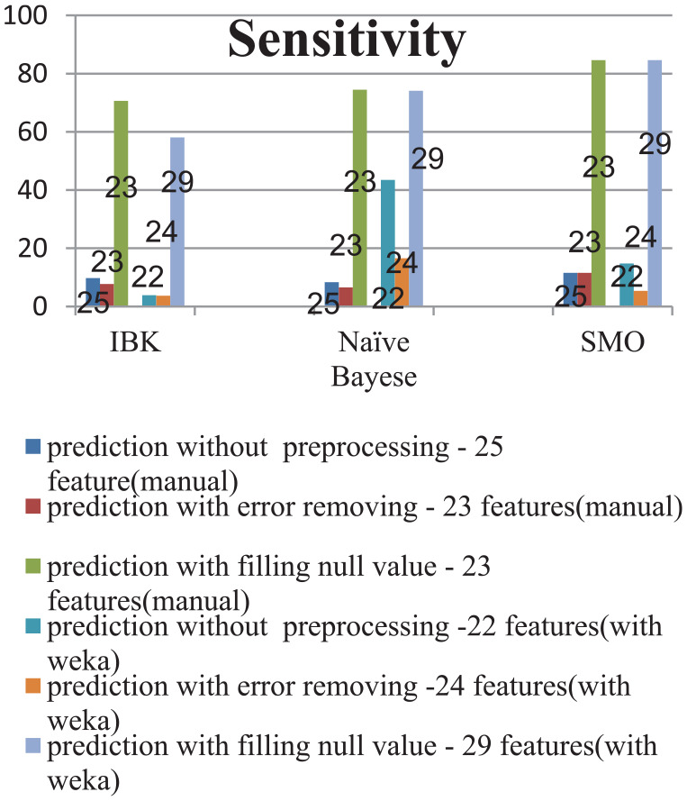
Comparing the sensitivity of the recurrence prediction models before and after preprocessing.

SMO indicates sequential minimal optimization.

Figure 5.

Comparing the precision of the recurrence prediction models before and after preprocessing.

SMO indicates sequential minimal optimization.

Figure 6.

Comparing F-measures of the recurrence prediction models before and after preprocessing.

SMO indicates sequential minimal optimization.

As can be seen in Figure 3, the accuracy measure has been improved in all algorithms after the step 3 of preprocessing. In terms of feature selection, in most algorithms of each step, the accuracy measure has the highest value in features selected manually. Moreover, among the 3 chosen classification algorithms, the SMO algorithm has shown the best performance in all steps of the case study.

Considering Figure 4, the sensitivity measure has been improved greatly after step 3 of preprocessing. In addition, after the third step of the case study, the algorithms SMO, naïve Bayes, and IBK showed the best performance, respectively.

According to Figure 5, the precision measure has been improved in most cases after data preprocessing, particularly after the step 3 of preprocessing which the precision measure has been improved greatly on all feature subsets. Furthermore, in most of the steps of the case study, the highest precision is especially for the manually selected feature subsets. Among the classification algorithms, the SMO algorithm has presented the best performance in all the steps.

As can be seen in Figure 6, F-measure has been greatly improved after the step 3 of preprocessing. In addition, the SMO algorithm has had the best performance in most cases.

Finally, considering Figure 7, G-mean has also been improved, like other measures, after the step 3 of preprocessing.

To investigate the significance of the difference in the steps of the case study, the analysis of variance (ANOVA; Welch) test was employed. In addition, in case of the significant result of the ANOVA (Welch) test, the Tukey (Tamhane) post hoc test was employed. According to the results presented in Tables 7 and 8, there were significant differences between the different steps of the case study in terms of accuracy, precision, sensitivity, F-measure, and G-mean measures (P < .001).

Table 7.

Comparing the results of 3 steps of the case study in terms of the sensitivity, precision, and G-mean measures.

P value	F	Standard deviation	Mean		Measure
<.001	82.88	12.27	21.56	Before preprocessing	Sensitivity
		11.29	18.46	Basic preprocessing
		16.03	69.57	Final preprocessing
<.001	34.19	21.51	29.88	Before preprocessing	Precision
		21.80	29.89	Basic preprocessing
		19.11	79.64	Final preprocessing
<.001	69.85	12.60	43.34	Before preprocessing	G-mean
		12.69	40.09	Basic preprocessing
		10.50	82.48	Final preprocessing

Table 8.

Comparing the 3 steps of the case study in terms of the F-measure and accuracy measures.

P value	W	Standard deviation	Mean		Measure
<.001	31.362	3.59	92.63	Before preprocessing	Accuracy
		2.68	93.35	Basic preprocessing
		1.37	97.88	Final preprocessing
<.001	80.126	8.41	20.17	Before preprocessing	F-measure
		8.48	18.74	Basic preprocessing
		17.04	73.85	Final preprocessing

Considering that the variances of the G-mean, sensitivity, and precision variables were the same in the 3 steps of the case study, the ANOVA test (Table 7) was used, and because of the inequality of the accuracy and F-measure variances throughout the 3 steps of the case study, the Welch test (Table 8) was used.

In terms of the results of the Tukey test, there was not any significant difference among the results of the prediction steps without preprocessing and with error removal; however, the prediction step with filling null values had a significant higher sensitivity, precision, and G-mean than the previous 2 steps.

Moreover, in terms of the results of the Tamhane test, the prediction steps without preprocessing and with error removal did not have any significant difference; however, the prediction step with filling null values had a significant higher accuracy and F-measure.

Considering the given results and interpretations, it is also necessary to note that there are many wide concepts in data preprocessing which entail the following challenges:

1. The different steps in the data preprocessing are interdependent and overlapping. For example, smoothing exists in the data cleaning and transformation. Also, aggregation and attribute construction exists in the data reduction and data transformation.²⁴

2. Data preprocessing deals with vast amounts of concepts and solutions, whose rearrangement affects the outputs. Therefore, it is not easy to claim that the best case, combination, and order have been considered in the preprocessing steps. For example, if the preprocessing is done with a different order, the results can be significantly different. After the data preprocessing is done, it may seem that the order of the steps is optimal, but there is an issue that other people may present a better solution.

With these explanations, many studies has been conducted in the field of breast cancer to predict the recurrence frequency, survival duration, diagnosis, etc, whose aim is to increase the accuracy of the prediction models, but besides increasing the accuracy of the prediction models, before applying any methodology, it should also be noted whether our data are of good quality, whether the data belong to our country’s population so that their results to be actually and practically applicable in medical decision-making, and whether the data are obsolete because if the data are too old and their treatment protocol is different from that used in the current time, the results cannot be used. However, by examining the numerous papers studied in this research, most of the studies have been done on simulated data. These kinds of data face less data preprocessing challenges because they are already preprocessed or their missing values and errors are very little. On the other hand, the preprocessing done in most papers have been only in 1 of the cases of missing values assignment, unbalanced data, dimension reduction, etc, while in this article a general process has been presented to select the appropriate preprocessing, and a combination of preprocessing steps has been done, in addition to using the related data of Iran.

Conclusions and Future Studies

In this article, a case study was conducted on the RROC breast cancer dataset. The case study was conducted in 3 steps of breast cancer recurrence prediction without preprocessing, breast cancer recurrence prediction with error removal, and breast cancer recurrence prediction with filling null values. The aim of this study was to examine the effect of preprocessing on data quality and the efficiency and performance of prediction models. As the results suggest, prediction by each of the 3 algorithms was improved after data preprocessing in terms of accuracy, sensitivity, precision, F-measure, and G-mean. The performance improvements were increased, respectively, 3.96%, 73.59%, 58.82%, 73.32%, and 58.85% for the SMO classifier; 12.04%, 66.54%, 72.74%, 66.48%, and 56.71% for the naïve Bayes classifier; and 5.76%, 60.9%, 71%, 65.57%, and 56.42% for the nearest neighbor classifier. Therefore, applying the appropriate preprocessing can improve the classification results and data quality. It should be noted that specialists of the RROC confirmed the validity of our procedure. So considering the careful investigations done in the case study, this study has the potential to be regarded as a guide to applying the appropriate preprocessing on the real-world data.

Considering the lessons learnt from the RROC dataset, the following are suggested:

1. Information about healthy participants in cancer screening should be gathered. Then, if some of these people refer to the center in the coming years because of cancer, a cancer prediction model will be developed using the data related to their healthy period and disease period. Then, using this model, the risk of cancer for healthy people is predicted and the required preventive measures undertaken.

2. Information about those patients with cancer no longer expected to be survived but miraculously (beyond the medical knowledge) fully recovered should be gathered from different hospitals of the country, with the hope that by gathering this information, a pattern is discovered and identified for the treatment of such patients with cancer.

3. In addition, by collecting information about family history of cancer in the patients, a model can be created based on which to predict the probability of getting cancer by the healthy individuals with a similar family history, and then the preventive measures are provided for them and the necessary advice is given to them.

References

- 1. Fan Q, Zhu CJ, Yin L. Predicting breast cancer recurrence using data mining techniques. In: 2010 International Conference on Bioinformatics and Biomedical Technology. New York, NY: IEEE; 2010:310-311. [Google Scholar]
- 2. Marzbani B, Nazari J, Najafi F, et al. Dietary patterns, nutrition, and risk of breast cancer: a case-control study in the west of Iran. Epidemiol Health. 2019; 41: e2019003. [DOI] [PMC free article] [PubMed] [Google Scholar]
- 3. Siegel Rebecca L, Miller Kimberly D, Jemal A. Cancer statistics, 2018. CA. 2018;68:7-30. [DOI] [PubMed] [Google Scholar]
- 4. Rathore N, Agarwal S. Predicting the survivability of breast cancer patients using ensemble approach. In: 2014 International Conference on Issues and Challenges in Intelligent Computing Techniques (ICICT). New York, NY: IEEE; 2014:459-464. [Google Scholar]
- 5. Hsu JL, Hung PC, Lin HY, Hsieh CH. Applying under-sampling techniques and cost-sensitive learning methods on risk assessment of breast cancer. J Med Syst. 2015;39:40. [DOI] [PubMed] [Google Scholar]
- 6. Ahmed AI, Hasan MM. A hybrid approach for decision making to detect breast cancer using data mining and autonomous agent based on human agent teamwork. In: 2014 17th International Conference on Computer and Information Technology (ICCIT). New York, NY: IEEE; 2014:320-325. [Google Scholar]
- 7. Zolbanin HM, Delen D, Zadeh AH. Predicting overall survivability in comorbidity of cancers: a data mining approach. Dec Supp Syst. 2015;74:150-161. [Google Scholar]
- 8. Liou DM, Chang WP. Applying data mining for the analysis of breast cancer data. In: Data Mining in Clinical Medicine. New York, NY: Humana Press; 2015:175-189. [DOI] [PubMed] [Google Scholar]
- 9. Karabatak M, Ince MC. An expert system for detection of breast cancer based on association rules and neural network. Exp Syst Appl. 2009;36:3465-3469. [Google Scholar]
- 10. Ghosh S, Mondal S, Ghosh B. A comparative study of breast cancer detection based on SVM and MLP BPN classifier. In: 2014 First International Conference on Automation, Control, Energy and Systems (ACES). New York, NY: IEEE; 2014:1-4. [Google Scholar]
- 11. Azmi MSBM, Cob ZC. Breast cancer prediction based on backpropagation algorithm. In: 2010 IEEE Student Conference on Research and Development (SCOReD). New York, NY: IEEE; 2010:164-168. [Google Scholar]
- 12. Sarvestani AS, Safavi AA, Parandeh NM, Salehi M. Predicting breast cancer survivability using data mining techniques. In 2010 2nd International Conference on Software Technology and Engineering. Vol. 2 New York, NY: IEEE; 2010:V2-227. [Google Scholar]
- 13. Han J, Micheline K. Data Mining: Concepts and Techniques. 2nd ed. Amsterdam, The Netherlands: Elsevier; 2006. [Google Scholar]
- 14. Salama GI, Abdelhalim M, Zeid MAE. Breast cancer diagnosis on three different datasets using multi-classifiers. Breast Cancer. 2012;32:2. [Google Scholar]
- 15. Fan CY, Chang PC, Lin JJ, Hsieh JC. A hybrid model combining case-based reasoning and fuzzy decision tree for medical data classification. Appl Soft Comput. 2011;11:632-644. [Google Scholar]
- 16. Ashraf M, Le K, Huang X. Iterative weighted k-NN for constructing missing feature values in Wisconsin breast cancer dataset. In: The 3rd International Conference on Data Mining and Intelligent Information Technology Applications. New York, NY: IEEE; 2011:23-27. [Google Scholar]
- 17. Chen CH. A hybrid intelligent model of analyzing clinical breast cancer data using clustering techniques with feature selection. Appl Soft Comput. 2014;20:4-14. [Google Scholar]
- 18. Purwar A, Singh SK. Hybrid prediction model with missing value imputation for medical data. Exp Syst Appl. 2015;42:5621-5631. [Google Scholar]
- 19. Santos V, Datia N, Pato MPM. Ensemble feature ranking applied to medical data. Proc Technol. 2014;17:223-230. [Google Scholar]
- 20. Peng Y, Wu Z, Jiang J. A novel feature selection approach for biomedical data classification. J Biomed Inform. 2010;43:15-23. [DOI] [PubMed] [Google Scholar]
- 21. Majid A, Ali S, Iqbal M, Kausar N. Prediction of human breast and colon cancers from imbalanced data using nearest neighbor and support vector machines. Comput Meth Prog Biomed. 2014;113:792-808. [DOI] [PubMed] [Google Scholar]
- 22. García-Laencina PJ, Abreu PH, Abreu MH, Afonoso N. Missing data imputation on the 5-year survival prediction of breast cancer patients with unknown discrete values. Comput Biol Med. 2015;59:125-133. [DOI] [PubMed] [Google Scholar]
- 23. Chapman P, Clinton J, Kerber R, et al. CRISP-DM 1.0: Step-by-step data mining guide. 2000. https://www.the-modeling-agency.com/crisp-dm.pdf.
- 24. Han J, Pei J, Kamber M. Data Mining: Concepts and Techniques. Amsterdam, The Netherlands: Elsevier; 2011. [Google Scholar]
- 25. Kerdegari H, Samsudin K, Ramli AR, Mokaram S. Evaluation of fall detection classification approaches. In: 2012 4th International Conference on Intelligent and Advanced Systems (ICIAS2012). Vol. 1 New York, NY: IEEE; 2012:131-136. [Google Scholar]
- 26. Chaurasia V, Pal S, Tiwari BB. Prediction of benign and malignant breast cancer using data mining techniques. J Algorith Comput Technol. 2018;12:119-126. [Google Scholar]
- 27. Sirageldin A, Baharudin BB, Jung LT. Malicious web page detection: a machine learning approach. In: Advances in Computer Science and its Applications. Berlin, Germany; Heidelberg, Germany: Springer; 2014:217-224. [Google Scholar]
- 28. Cufoglu A, Lohi M, Madani K. A comparative study of selected classifiers with classification accuracy in user profiling. In: 2009 WRI World Congress on Computer Science and Information Engineering. Vol. 3 New York, NY: IEEE; 2009:708-712. [Google Scholar]
- 29. Selvakuberan K, Indradevi M, Rajaram R. Combined feature selection and classification – a novel approach for the categorization of web pages. J Inform Comput Sci. 2008;3:83-89. [Google Scholar]
- 30. Khonji M, Jones A, Iraqi Y. An empirical evaluation for feature selection methods in phishing email classification. Int J Comput Syst Sci Eng. 2013;28:37-51. [Google Scholar]
- 31. Witten LH, Frank E, Hall MA. Data Mining Practical Tools and Techniques. 3rd ed. San Francisco, CA: Morgan Kaufmann Publishers; 2011. [Google Scholar]
- 32. Gnanambal S, Thangaraj M, Meenatchi VT, Gayathri V. Classification algorithms with attribute selection: an evaluation study using WEKA. Int J Adv Netw Appl. 2018;9:3640-3644. [Google Scholar]
- 33. Peng Y, Wang G, Wang H. User preferences based software defect detection algorithms selection using MCDM. Inform Sci. 2012;191:3-13. [Google Scholar]
- 34. He H, Garcia EA. Learning from imbalanced data. IEEE Trans Knowl Data Eng. 2008;9:1263-1284. [Google Scholar]
- 35. Nivetha S, Samundeeswari ES. Predicting survival of breast cancer patients using fuzzy rule based system. Int Res J Eng Technol. 2016;3:962-969. [Google Scholar]