Theory of Diffusion-Influenced Reaction Networks

Abstract

A formalism is developed to describe how diffusion alters the kinetics of coupled reversible association-dissociation reactions in the presence of conformational changes that can modify the reactivity. The major difficulty in constructing a general theory is that, even to lowest order, diffusion can change the structure of the rate equations of chemical kinetics by introducing new reaction channels (i.e., modifies the kinetic scheme). Therefore, the right formalism must be found that allows the influence of diffusion to be described in a concise and elegant way for networks of arbitrary complexity. Our key result is a set of non-Markovian rate equations involving stoichiometric matrices and net reaction rates (fluxes), in which these rates are coupled by a time-dependent pair association flux matrix, whose elements have a simple physical interpretation. Specifically, each element is the probability density that an isolated pair of reactants irreversibly associates at time t via one reaction channel on condition that it started out with the dissociation products of another (or the same) channel. In the Markovian limit, the coupling of the chemical rates is described by committors (or splitting/capture probabilities). The committor is the probability that an isolated pair of reactants formed by dissociation at one site will irreversibly associate at another rather than diffuse apart. We illustrate the use of our formalism by considering three reversible reaction schemes: (1) binding to a single site, (2) binding to two inequivalent sites, and (3) binding to a site whose reactivity fluctuates. In the first example, we recover the results published earlier, while in the second one we show that a new reaction channel appears, which directly connects the two bound states. The third example is particularly interesting because all species become coupled and an exchange-type bimolecular reaction appears. In the Markovian limit, some of the diffusion-modified rate constants that describe new transitions become negative, indicating that memory effects cannot be ignored even in an approximate description.

Graphical Abstract

I. Introduction

Our understanding of how the diffusive motion of the reactants influences kinetics started with the seminal work of Smoluchowski¹ on irreversible reactions more than a hundred years ago. The generalization to reversible diffusion-influenced reactions is a challenging many-body problem that has been attacked by many people from different directions using a variety of approaches.^2–36 For simple reactions like A+B ⇌ C and A+B ⇌ C+D, a consensus has been reached on as to what is the simplest theory that (1) reduces to the rate equations of chemical kinetics when diffusion is fast, (2) is exact at short times and asymptotically (i.e., gives the correct amplitude of the power law relaxation to equilibrium), and (3) is exact in the geminate limit (i.e., for the reversible reaction of an isolated pair of particles).

Some time ago, we found a concise formulation of this consensus theory for A+B ⇌ C and A+B ⇌ C+D and discussed various extensions to improve the performance at intermediate times.²³ While the exact diffusion-influenced rate equations can be formally written in terms of the pair distribution functions of reactants, these functions do not satisfy a closed set of equations. Our approach was based on approximate equations for the deviation of these functions from their bulk values, which are in some sense smaller than the pair distribution functions themselves. These equations describe how the deviations change due to diffusion and reaction between the molecules forming the pair as well as with molecules in the bulk. However, we did not consider an explicit form of the diffusion-influenced rate equations for a network of reversible reactions of arbitrary complexity.

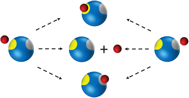
The difficulty in formulating such a general theory is that diffusion can modify the structure of the rate equations of chemical kinetics by introducing new reaction channels not present in the original kinetic scheme. We found this recently^33,35 in the context of multisite phosphorylation where an enzyme can modify a substrate at several sites.³⁷ The physical reason can be most easily seen for reversible ligand binding to a macromolecule with two inequivalent sites (Figure 1(a)) or to a macromolecule that fluctuates between conformations with different binding sites (see Figure 1(b)). In the first case, a ligand that has dissociated form one site can directly rebind to the other site rather than diffuse away into the bulk (the upper pathway in Figure 1(a)). This process would never occur if diffusion were very fast and hence is not included in ordinary chemical kinetics, which considers only the lower reaction pathway in Figure 1(a). Thus diffusion induces a direct transition between the two bound states. The situation is similar in the second example, where a ligand that just dissociated from the binding site of one conformation can directly rebind to a different site of the other conformation when a conformational transition has occurred before the ligand could diffuse away into the bulk (the upper pathway in Figure 1(b)). As we shall see later, this process induces all kinds of new reaction channels.

Figure 1:

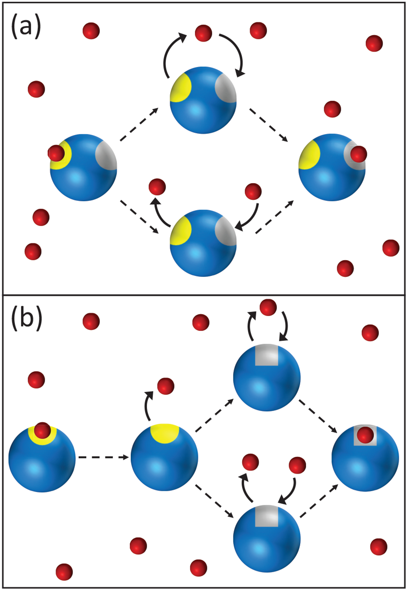
Effect of diffusion on ligand binding when the ligands (red) are in excess. (a) After dissociation from one site of a macromolecule, the ligand can bind to the same (yellow) site or to the second (gray) site (upper pathway). Alternatively, another ligand from the bulk can bind (lower pathway). In the lower pathway, the macromolecule and the ligand that binds to the second site are uncorrelated, and this pathway corresponds to the conventional chemical kinetics. In the upper pathway, the macromolecule and the ligand are correlated. This leads to an additional reaction channel between two (left and right) bound states. (b) Same for ligand binding to a site with fluctuating reactivity (yellow and gray).

In this paper our starting point is the set of rate equations of chemical kinetics written in terms of reaction rates and stoichiometric coefficients, which is widely used to describe biochemical networks.³⁸ Our main result is a set of non-Markovian diffusion-modified rate equations, in which the bimolecular chemical rates are coupled by a time-dependent matrix of pair association fluxes. The calculation of these fluxes requires the solution of an irreversible pair, rather than a many-body, problem. An element of the matrix of association fluxes is the probability density that, starting with the dissociation product of one reaction channel, irreversible binding occurs at time t via another (or the same for the diagonal elements) reaction channel. In the Markovian limit, each flux is replaced by a committor or splitting/capture probability,^39–41 which is the probability that a pair of reactants, just formed by dissociation of a complex, eventually irreversibly associate to form another (or the same) complex. The simple structure of our diffusion-modified rate equations, where the chemical reaction rates are just coupled, can, in general, hide an underlying complexity that emerges when one examines the corresponding kinetic schemes and finds new reaction channels that were absent in the original chemical rate equations.

We illustrate how our formalism can be used by considering three examples. The first example is single-site binding, A+B ⇌ C. Using our general theory in this well-studied case is like using sledgehammer to crack a nut. Nevertheless, we hope that it will provide some physical insight. In the second example, a ligand can bind to two inequivalent sites to form two different complexes. This is related to double phosphorylation, where an enzyme can modify the substrate at two different sites. Within the framework of our formalism, diffusion just couples the two chemical reaction rates (or fluxes) corresponding to association-dissociation at the two sites. A consequence of this simple coupling is that a new reaction channel is introduced into the kinetic scheme, in which two complexes can directly interconvert. In the last example, we consider reversible binding to a macromolecule that fluctuates between two conformations with different reactivity. The most surprising result is that in the Markovian, or steady-state, limit, not all rate constants that describe new diffusion-induced transitions are positive.

II. The rate equations of chemical kinetics

Consider species X_i, i = 1, 2, …, N_s, that can undergo bimolecular association-dissociation reactions, X_m+X_n ⇌ X_l and, possibly, reversible unimolecular reactions, X_m ⇌ X_n. For the sake of simplicity we do not consider the case when m = n and exchange-type reactions,^20,42 X_m +X_n ⇌ X_i +X_j, but our formalism can easily be extended to handle such reactions. We also do not consider trimolecular reactions because the diffusive encounter of three molecules is rare in dilute solutions.

A. Reaction rates and stoichiometric matrices

In the limit that diffusion is sufficiently fast (the reaction-controlled limit), the time evolution of the concentrations is described by the ordinary rate equations of chemical kinetics. Here we adopt a representation that involves stoichiometric matrices and net reaction rates or fluxes, which has been used to describe metabolic reaction networks.³⁸ For the unimolecular reaction X_m ⇌ X_n, the net reaction rate is denoted by

$$u_{mn}={\kappa }_{m\to n}\left[X_m\right]-{\kappa }_{n\to m}\left[X_n\right]$$ (2.1)

where [X_i] is the concentration of species X_i and κ_i→j is the rate constant describing the transition X_i → X_j. For the bimolecular reaction X_m + X_n ⇌ X_l, the net reaction rate is denoted by

$$v_{mnl}={\kappa }_{mn\to l}\left[X_m\right]\left[X_n\right]-{\kappa }_{l\to mn}\left[X_l\right]$$ (2.2)

where κ_mn→l (κ_l→mn) is the intrinsic association (dissociation) rate constant. We have combined the forward and reverse reaction rates, so these net rates vanish at equilibrium. The number of unimolecular and bimolecular reactions is denoted as N_u and N_b, respectively. The number of species is denoted as N_s.

Let x(t) be the vector of species concentrations so that x_i = [X_i], i = 1, 2, …, N_s. Then the rate equations of chemical kinetics can be written in terms of the uni- and bimolecular rates as

$$\frac{dx}{dt}=S_{1}u+S_{2}v$$ (2.3)

Here u (v) is the vector of non-zero uni(bi)molecular rates with N_u (N_b) elements and S₁ (S₂) are the uni(bi)molecular stoichiometric matrices with non-zero elements that are the stoichiometric coefficients. For example, for the unimolecular reaction X₁ ⇌ X₂, these coefficients are −1 and 1, while for X₁ + X₂ ⇌ X₃ they are −1, −1, and 1. The rows of a stoichiometric matrix represent species and the columns represent reactions. Thus S₁ is a rectangular matrix of size N_s × N_u and the bimolecular stoichiometric matrix S₂ has size N_s × N_b. Note that the summation in the matrix-vector multiplication in eq 2.3 is performed over reactions, not species. We have introduced separate stoichiometric matrices for uniand bimolecular reactions because it turns out that diffusion modifies only the bimolecular net rates.

B. Linearized rate equations

The above rate equation is nonlinear but it can be linearized about equilibrium. Let δ[X_n] = [X_n(t)] − [X_n]_eq be the deviation of the concentration of species X_n from its equilibrium value, lim_t→∞[X_n(t)] = [X_n]_eq. If we substitute [X_n(t)] = δ[X_n(t)] + [X_n]_eq into eqs 2.1 and 2.2 and neglect the quadratic term δ[X_m]δ[X_n], then it can be shown, using eq 2.3, that the vector of concentration deviations, δx = x − x_eq, satisfies

$$\frac{d\delta x}{dt}=K\delta x$$ (2.4)

where K is an N_s × N_s square matrix with elements

$$K_{ij}=\underset{t\to \infty }{\text{lim}}\frac{\partial }{\partial \left[X_j\right]}\left(\frac{d\left[X_i\right]}{dt}\right)={\left[K_1\right]}_{ij}+\underset{t\to \infty }{\text{lim}}\frac{\partial }{\partial \left[X_j\right]}{\left(S_{2}v\right)}_i$$ (2.5)

Here K₁ is the rate matrix that describes unimolecular transitions, [K₁]_ij = κ_j→i, i ≠ j, and ${\left[K_1\right]}_{ii}=-{\sum }_{j=1}^{N_u}{\kappa }_{i\to j}$. The elements of the linearized matrix K are the sums of the unimolecular and bimolecular reaction terms. Because of the presence of bimolecular reactions, the matrix K depends on the equilibrium concentrations. The matrix elements of K satisfy the detailed balance condition:

$$K_{ij}{\left[X_j\right]}_{eq}=K_{ji}{\left[X_i\right]}_{eq}$$ (2.6)

which follows from detailed balance for each reaction, [X_i]_eqκ_i→j = [X_j]_eqκ_j→i, [X_i]_eq[X_j]_eqκ_ij→l = [X_l]_eqκ_l→ij.

For future reference, let us consider how correlations between the concentration deviations from equilibrium evolve in time in the framework of chemical kinetics. Let $\delta {\mathcal{P}}_{CH}$ be a matrix with elements ${\left[\delta {\mathcal{P}}_{CH}\right]}_{ij}=\delta \left[X_i\right]\delta \left[X_j\right]=\left(\left[X_i\right]-{\left[X_i\right]}_{eq}\right)\left(\left[X_j\right]-{\left[X_j\right]}_{eq}\right)$. Then it can be shown, using eq 2.4, that

$$\frac{d}{dt}\delta {\mathcal{P}}_{CH}=K\delta {\mathcal{P}}_{CH}+\delta {\mathcal{P}}_{CH}{K}^{\top }$$ (2.7)

where K^⊤ is the transpose of the linearized matrix K.

III. Influence of diffusion on the kinetics: General theory

In this section we will show that the influence of diffusion on the time evolution of the concentrations can be described by

$$\frac{dx}{dt}=S_{1}u+S_2\left(v-{\int }_0^{t}J\left(t-t\prime \right)v\left(t\prime \right)dt\prime \right)$$ (3.1)

This non-Markovian equation with memory is to be compared with the rate equation of ordinary chemical kinetics given in eq 2.3. Note that, since at equilibrium all the v’s are zero, both equations lead to the same equilibrium concentrations. Here an element of the N_b × N_b flux matrix J(t) is the probability density that an isolated pair irreversibly associates at time t via one reaction channel having started out with the dissociation product of the same or another channel. For three-dimensional systems, the Markovian limit of eq 3.1 is

$$\frac{dx}{dt}=S_1\mathit{\text{u}}+S_2\left(\mathit{\text{I}}-\mathit{\text{Q}}\right)v$$ (3.2)

where I is the unit matrix of size N_b and

$$\mathit{\text{Q}}={\int }_0^{\infty }\mathit{\text{J}}\left(t\right)dt$$ (3.3)

An element of the committor matrix Q is the probability that the dissociation products of one reaction channel irreversibely associate via another (or the same) channel rather than diffusing apart. The committor or splitting or capture probability was introduced by Onsager³⁹ in the context of ion-pair recombination and its role in simple reactions like A+B ⇌ C has been known for a long time.⁴¹ It also plays a central role in modern theories of unimolecular reactions on free energy surfaces (e.g., see references^43–46).

We will derive these results for the following microscopic model of the association of two molecules X_m and X_n to form a complex X_l and the dissociation of this complex to form X_m and X_n. Assume for the sake of simplicity that there is no interaction potential between X_m and X_n other than a short-range repulsive one. Instead of describing reactivity by using boundary conditions at contact, we will use more general “sink” functions. Let us denote the relative distance and the orientations of the two reactants by a “generalized” coordinate r. At each r, we assume that X_m and X_n can form X_l with a “unimolecular” rate constant κ_mn→lσ_mnl(r), i.e., the lifetime of an X_m − X_n pair is 1/(κ_mn→lσ(r)). The normalized sink function ${\sigma }_{mnl}(r)\left(\int {\sigma }_{mnl}(r)dr=1\right)$ is nonzero only in the region of conformational space where X_m and X_n have the appropriate separation and orientations to form a stereospecific complex. Since X_m and X_n may have several binding sites, they can form different complexes and this is why the sink function is also labelled by the index l. The complex X_l can dissociate with unimolecular rate constant κ_l→mn to form X_m and X_n with relative separation and orientations r chosen from the probability distribution σ_mnl(r). The spatial and orientational dependence of σ_mnl(r) for association and dissociation must be the same because of detailed balance.

A. The exact rate equations for the concentrations

The diffusion-influenced rate equations for the bulk concentrations can be expressed in terms of the time-dependent pair distribution functions (or, reduced distribution functions^47,48) ρ_mn. The function ρ_mn(r₁, r₂, t) is the joint probability density for finding a molecule X_m at r₁ and any other molecule X_n at r₂ at time t. For a homogeneous system, this function depends on the distance between the two molecules and their orientations, r. As the relative distance becomes large, the molecules become uncorrelated and ρ_mn(r, t) approaches [X_m(t)][X_n(t)] (i.e., the product of the bulk concentrations). The influence of diffusion on the kinetics can be accounted for by simply replacing the association rate in chemical kinetics

(i.e., κ_mn→l[X_m][X_n]) by ${\kappa }_{mn\to l}\int {\sigma }_{mnl}(r){\rho }_{mn}(r,t)dr$ in eq 2.2. The resulting equations are exact for a homogeneous system as long as the pair distribution functions are exact. Thus the diffusion-influenced rate equation can be written as (see eq 2.3)

$$\frac{dx}{dt}=S_1\mathit{\text{u}}+S_2\mathit{\text{w}}$$ (3.4)

where w is the vector of the diffusion-influenced reaction rates defined as

$$\begin{gathered} w_{mnl}\equiv {\kappa }_{mn\to l}\int {\sigma }_{mnl}\left(\mathit{\text{r}}\right){\rho }_{mn}\left(\mathit{\text{r}},t\right)d\mathit{\text{r}}-{\kappa }_{l\to mn}\left[X_l\left(t\right)\right] \\ =v_{mnl}+{\kappa }_{mn\to l}\int {\sigma }_{mnl}\left(\mathit{\text{r}}\right)\delta {\rho }_{mn}\left(\mathit{\text{r}},t\right)d\mathit{\text{r}} \end{gathered}$$ (3.5)

where we used $\int {\sigma }_{mnl}\left(\mathit{\text{r}}\right)d\mathit{\text{r}}=1$. Here δρ_mn(r, t) is the deviation of the pair distribution function from its bulk value

$$\delta {\rho }_{mn}\left(\mathit{\text{r}},t\right)={\rho }_{mn}\left(\mathit{\text{r}},t\right)-\left[X_m\left(t\right)\right]\left[X_n\left(t\right)\right]$$ (3.6)

Note that diffusion has no influence on the unimolecular rates (compare eqs 2.3 and 3.4). If ρ_mn(r, t) in eq 3.5 were replaced by its large distance limit, [X_m][X_n], then w_mnl would reduce to the chemical kinetics rate v_mnl since δρ_mn = 0.

B. Approximate equations for the pair distribution function

To make progress, one must determine the pair distribution functions ρ_mn(r, t) or, equivalently, the deviations from the bulk values, δρ_mn(r, t). Herein lies the difficulty of the problem because no closed equation exists for these functions. Instead they satisfy an infinite hierarchy of equations where the equation for the n-particle distribution function involves the (n + 1)-particle one.⁴⁸ One approach is to truncate this hierarchy with a possibly uncontrolled approximation. Here we take a more physically intuitive approach by constructing an approximate equation for deviation of the pair distribution function from its bulk value that accounts in a simple way for all processes that can change this function. These include (1) diffusion, (2) direct reaction of the reactants in the pair X_m − X_n (i.e., the pair may disappear due to association and appear due to dissociation of a complex), (3) unimolecular interconversion and (4) the reaction of one of the reactants in the pair with another molecule in the bulk.

Let us start with diffusion because this is the simplest. In the absence of reaction and rotational diffusion, δρ_mn would satisfy

$$\frac{\partial }{\partial t}\delta {\rho }_{mn}\left(\mathit{\text{r}},t\right)=\left(D_m+D_n\right){\nabla }^2\delta {\rho }_{mn}$$ (3.7)

where D_i is the translational diffusion constant of X_i and D_m + D_n is the relative diffusion constant of X_m and X_n. This equation can be readily generalized to include rotational dynamics of X_m and X_n, but this would lead to unnecessary complications in the notation. If we introduce an N_s × N_s square matrix of deviations $\delta \mathcal{P}(\mathit{\text{r}},t)$ with elements $\delta {\mathcal{P}}_{mn}=\delta {\rho }_{mn}=\delta {\mathcal{P}}_{nm},$, then the above equation can be rewritten in matrix notation as

$$\frac{\partial }{\partial t}\delta \mathcal{P}\left(\mathit{\text{r}},t\right)={\nabla }^2\left(\mathit{\text{D}}\delta \mathcal{P}+\delta \mathcal{P}\mathit{\text{D}}\right)$$ (3.8)

where D is a diagonal matrix with the diffusion coefficients on the diagonal.

To describe the influence of the association-dissociation reaction between X_m and X_n, we must modify eq 3.7 by subtracting the rate at which an X_m − X_n pair disappears due to association and add the rate at which it appears due to the dissociation of X_l. This can be done by subtracting F_mn from the right-hand side of eq 3.7, where

$$F_{mn}\left(\mathit{\text{r}},t\right)=\sum _l\left({\kappa }_{mn\to l}{\rho }_{mn}\left(\mathit{\text{r}},t\right)-{\kappa }_{l\to mn}\left[X_l\right]\right){\sigma }_{mnl}\left(\mathit{\text{r}}\right)$$ (3.9)

Here the sum over l accounts for the possibility that X_m and X_n can form different complexes as, for example, when there are multiple binding sites.

Equation 3.9 can be rewritten in terms of the chemical kinetics bimolecular rate v_mnl(t) defined in eq 2.2:

$$F_{mn}\left(\mathit{\text{r}},t\right)=R_{mn}^{irr}\left(\mathit{\text{r}}\right)\delta {\rho }_{mn}\left(\mathit{\text{r}},t\right)+V_{mn}\left(\mathit{\text{r}},t\right)$$ (3.10)

where we have defined

$$R_{mn}^{irr}\left(\mathit{\text{r}}\right)=\sum _l{\kappa }_{mn\to l}{\sigma }_{mnl}\left(\mathit{\text{r}}\right)$$ (3.11a)

$$V_{mn}\left(\mathit{\text{r}},t\right)=\sum _l{v}_{mnl}\left(t\right){\sigma }_{mnl}\left(\mathit{\text{r}}\right)$$ (3.11b)

Thus, in matrix notation, so far we have

$$\frac{\partial }{\partial t}\delta \mathcal{P}\left(\mathit{\text{r}},t\right)={\nabla }^2\left(\mathit{\text{D}}\delta \mathcal{P}+\delta \mathcal{P}\mathit{\text{D}}\right)-R^{irr}\circ \delta \mathcal{P}-\mathit{\text{V}}$$ (3.12)

where ○ denotes the element-wise (Hadamard) product (i.e., [A○B]_ij = A_ijB_ij), R^irr and V are N_s × N_s matrices with the elements $R_{mn}^{irr}(\mathit{\text{r}})$ and V_mn(r, t), respectively. The superscript “irr” means “irreversible” because this matrix involves only the association rate constants. In the next step we consider the changes in the pair distribution functions due to unimolecular reactions. Consider an X_m − X_n pair. If X_n is unimolecularly converted into X_i, then the X_m − X_n pair is converted into a X_m − X_i pair. Similarly, if X_m becomes X_i, then the X_m − X_n pair is converted into the X_i − X_n pair. Thus δρ_mn, δρ_mi, and δρ_in are coupled. To describe this, we add the terms ${\sum }_i\left({\kappa }_{i\to m}\delta {\rho }_{in}+{\kappa }_{i\to n}\delta {\rho }_{mi}-\left({\kappa }_{m\to i}+{\kappa }_{n\to i}\right)\delta {\rho }_{mn}\right)$ to the equation for δρ_mn. In matrix form, this is equivalent to adding a term $K_1\delta \mathcal{P}+\delta \mathcal{P}{K}_1^{\top }$ eq 3.12 (similar to eq 2.7), where the matrix K₁ is the rate matrix of unimolecular transitions with the elements ${\left[K_1\right]}_{ij}={\kappa }_{j\to i},{\left[K_1\right]}_{ii}=-{\sum }_j{\kappa }_{i\to j}$. Finally, we account for the changes in the pair distribution functions due to reaction with bulk molecules (i.e., the molecules that are not involved in a specific pair). For example, suppose that X_m reacts with a molecule from the bulk and forms the complex X_l (see Figure 2). This converts the X_m − X_n pair into the X_l − X_n pair, coupling δρ_mn with δρ_ln. The simplest, but of course approximate, way to quantitatively account for this process is to describe it in the framework of chemical kinetics linearized near equilibrium. To do this, all we have to do is to add a term $K\delta \mathcal{P}+\delta \mathcal{P}{K}^{\top }$ to eq 3.12 (see eq 2.7), where the matrix K is given in eq 2.5. In this way, we account for changes due to both unimolecular reactions and reactions with bulk molecules. Thus we have

$$\frac{\partial }{\partial t}\delta \mathcal{P}\left(\mathit{\text{r}},t\right)={\nabla }^2\left(\mathit{\text{D}}\delta \mathcal{P}+\delta \mathcal{P}\mathit{\text{D}}\right)+\mathit{\text{K}}\delta \mathcal{P}+\delta \mathcal{P}{\mathit{\text{K}}}^{\top }-{\mathit{\text{R}}}^{irr}\circ \delta \mathcal{P}-\mathit{\text{V}}$$ (3.13)

This equation completely determines δρ_mn and hence the diffusion-influenced reaction rate w_mnl in eq 3.5. This rate can then be used to find the time dependence of the bulk concentrations via eq 3.4. Equation 3.13 must be solved subject to reflecting boundary conditions when two molecules are in contact. Since all molecules are assumed to be initially uniformly distributed, it must be solved subject to the initial condition that δρ_mn(r, 0) = 0. Consequently, at short times w_mnl = v_mnl (see eq 3.5) and conventional chemical kinetics is accurate.

Figure 2:

Effect of bulk reaction on δρ_mn for X_m + X_n ⇌ X_l. An X_m − X_n pair is coupled with X_l − X_n pair due to binding of an X_n molecule from the bulk (dashed red) to X_m.

Considering its generality, eq 3.13 has a simple structure. The first two terms in the right-hand side describe changes in the deviation of the pair distribution function from its bulk value due to diffusion. The next two terms describe changes due to unimolecular reactions and to bimolecular reactions with molecules in the bulk when the system is near equilibrium. The last two terms describe the changes due to association of the reactants in a pair and the dissociation of a complex to form a new pair.

We believe that the above formalism is the simplest one that accurately describes the kinetics both at short and long times. Because of diffusion, the kinetics at long times is not exponential but rather a power law.^24,49,50 We have proved that for A + B ⇌ C the above equation leads to the exact asymptotics²³ and conjecture that this is true for any system where the equilibrium concentrations are finite. At low concentrations, eq 3.13 can be simplified by retaining only the unimolecular contributions to K, but the resulting asymptotics will no longer be exact. Finally, we believe that eq 3.13 could be formally derived by truncating the infinite hierarchy satisfied by the n-particle distribution functions using a linearized superposition approximation (i.e., approximately expressing the three-particle distribution function in terms of pair distributions). We have explicitly shown this for the reaction A + B ⇌ C, A ⇌ D.³⁶ In addition, for A + B ⇌ C, we derived this in a rather complicated way²⁴ by starting with the Poisson representation⁵¹ of the master equation for a large number of reacting particles jumping on a lattice.

Equation 3.13 can be improved in a number of ways while retaining its structure. The linearized matrix K involves the intrinsic association (κ_mn→l) and dissociation (κ_l→mn) rate constants which do not depend on diffusion. One can replace them with effective diffusion-influenced rate constants that can be chosen in a number of ways as discussed later in this paper. In addition, K contains the equilibrium concentrations. This is satisfactory at long times and does not matter at short times where the deviation of the pair distribution is zero. To increase the accuracy at intermediate times, it would be preferable to replace the equilibrium concentrations by their instantaneous bulk concentrations. However, this would make the matrix K time dependent, K → K(t), and make eq 3.13 much more difficult to solve.

C. Solution of the equation for the pair distribution functions

The equation that determines the pair distribution functions, eq 3.13, involves the time-dependent reaction rates (through V defined in eq 3.11b) which also enter into the rate equations that determine the time dependence of the bulk concentrations via eqs 3.4 and 3.5. This difficulty can be bypassed by introducing a Green’s function that satisfies an equation similar to eq 3.13, but without V. Let G_mn,m′n′(r, t | r′, t′) be the solution of

$$\frac{\partial }{\partial t}\mathit{\text{G}}\left(\mathit{\text{r}},t\right)={\nabla }^2\left(DG+GD\right)+KG+G{K}^{\top }-{\mathit{\text{R}}}^{irr}\circ G$$ (3.14)

where G is an N_b × N_b matrix with elements G_mn(r, t), subject to the initial condition G_mn(t = t′) = (δ_mm′δ_nn′ +δ_mn′δ_nm′)δ(r − r′) (m′ ≠ n′). Here δ(r − r′) is the Dirac δ-function and δ_ij is the Kronecker delta, δ_ij = 1 when i = j and zero otherwise. This initial condition insures that the Green’s function is symmetric in both m and n and m′ and n′ since there is no difference for instance between an X_m − X_n and X_n − X_m pair. This Green’s function describes pair dynamics due to diffusion, irreversible association, unimolecular transitions, and reaction with bulk molecules.

The solution of eq 3.13 can now be written as

$$\delta {\rho }_{mn}\left(\mathit{\text{r}},t\right)=-\sum _{m\prime <n\prime }{\int }_0^{t}dt\prime \int d\mathit{\text{r}}\prime G_{mn,m^{\prime }{n}^{\prime }}\left(\mathit{\text{r}},t|\mathit{\text{r}}\prime ,t\prime \right)V_{m^{\prime }{n}^{\prime }}\left(\mathit{\text{r}}\prime ,t\prime \right)$$ (3.15)

since V is an inhomogeneous term independent of the δρ’s. This can be verified by direct substitution of eq 3.15 into eq 3.13. Substituting δρ_mn in eq 3.15 into eq 3.5 and using the definition of V_mn in eq 3.11b we find that the diffusion-influenced net reaction rates are

$$w_{mnl}\left(t\right)=v_{mnl}\left(t\right)-\sum _{m\prime <n\prime ,l\prime }{\int }_0^t{J}_{mnl,m\prime n\prime l\prime }\left(t-t\prime \right)v_{m\prime n\prime l\prime }\left(t\prime \right)dt\prime$$ (3.16)

where we have defined pair association fluxes as

$$J_{mnl,m\prime n\prime l\prime }\left(t\right)={\kappa }_{mn\to l}\int {\sigma }_{mnl}\left(\mathit{\text{r}}\right)G_{mn,m\prime n\prime }\left(\mathit{\text{r}},t|\mathit{\text{r}}\prime ,0\right){\sigma }_{m\prime n\prime l\prime }\left(\mathit{\text{r}}\prime \right)d\mathit{\text{r}}d\mathit{\text{r}}\prime$$ (3.17)

The physical meaning of J_{mnl,m′n′l′}(t) will be considered later. These quantities are not all independent because of detailed balance condition in eq 2.6. It can be shown that the detailed balance condition for the J’s is

$$J_{mnl,m\prime n\prime l\prime }\left(t\right){\kappa }_{m\prime n\prime \to l\prime }{\left[X_{m\prime }\right]}_{eq}{\left[X_{n\prime }\right]}_{eq}=J_{m\prime n\prime l\prime ,mnl}\left(t\right){\kappa }_{mn\to l}{\left[X_m\right]}_{eq}{\left[X_n\right]}_{eq}$$ (3.18)

D. Diffusion-modified rate equations

The number of unique non-zero net reaction rates, w_mnl(t) or v_mnl(t), is equal to the number of different bimolecular reaction channels, N_b. If we label reaction channels by α, α = 1, 2, …, N_b, then we can replace the summation over m′, n′ and l′ in eq 3.16 by the summation over the reaction channels α′. Therefore, the equation for the diffusion-influenced reaction rate, eq 3.16, can be nicely written in matrix form

$$w\left(t\right)=v\left(t\right)-J\left(t\right)*v\left(t\right)$$ (3.19)

where J(t) * v(t) denotes the convolution ${\int }_0^{t}J\left(t-t^{\prime }\right)v\left(t^{\prime }\right)d{t}^{\prime }$ and J(t) is an N_b × N_b square matrix with elements J_α,α′ ≡ J_{mnl,m′n′l′} defined in eq 3.17. This matrix couples channels α (X_m +X_n ⇌ X_l) and α′ (X_m′ +X_n′ ⇌ X_l′). The diffusion-influenced rate equation in eq 3.4 can now be written in a compact way

$$\frac{dx}{dt}=S_1\mathit{\text{u}}+S_2\left(v-\mathit{\text{J}}\left(t\right)*\mathit{\text{v}}\left(t\right)\right)$$ (3.20)

The summations in the matrix-vector and matrix-matrix multiplications are performed with respect to the reaction channels. This is the key result of the theory as previously presented in eq 3.1. The time dependence of the bulk concentrations is determined by the fluxes J’s that can be found by solving a two-particle problem involving pairs that can irreversibly associate. The unimolecular reaction rate u’s are not modified by diffusion. If diffusion were very fast then all these J’s would be zero because the initial pair would diffuse apart and never react, and hence eq 3.20 would reduce to the rate equations of ordinary chemical kinetics, eq 2.3.

E. Markovian approximation

When pair association fluxes J(t) change much faster than the bulk reaction rates, v(t), then the convolution in eq 3.20, ${\int }_0^{t}J\left(t-t^{\prime }\right)v\left(t^{\prime }\right)d{t}^{\prime }$, can be approximated by $\left({\int }_0^{\infty }J\left(t^{\prime }\right)d{t}^{\prime }\right)v(t)$ and hence the diffusion-influenced rate equations can be written as (see also eq 3.2)

$$\frac{dx}{dt}=S_1\mathit{\text{u}}+S_2\left(\mathit{\text{I}}-\mathit{\text{Q}}\right)\mathit{\text{v}}$$ (3.21)

where I is the N_b × N_b unit matrix and $Q={\int }_0^{\infty }J(t)dt$ as in eq 3.3. When the Q matrix is diagonal, the diffusion-influenced rate equations are obtained by simply multiplying both intrinsic association and dissociation rate constant, κ_mn→l and κ_l→mn, by (1 − Q_mnl,mnl) (compare eqs 3.21 and 2.2–2.3).

F. Physical Interpretation of pair association fluxes and committors

The physical meaning of J’s and Q’s is transparent when the linearized matrix K is actually a rate matrix, i.e., satisfies ${\sum }_m{K}_{mn}=0$. This is true for unimolecular reactions and for bimolecular reactions that are pseudo-first order. In this case the Green’s function G_mn,m′n′ describes two diffusing molecules that can associate irreversibly and change their states with rate constant K_ij (see eq 3.14). Specifically, G_mn,m′n′(r, t | r′, t′) is the probability density that an X_m′ −X_n′ pair that is separated by r′ at time t′ becomes the pair X_m − X_n separated by r at time t. The initial X_m′ − X_n′ pair can convert into X_m − X_n because of unimolecular transitions X_m′ → X_m and X_n′ → X_n and/or because of reaction with the bulk, as described by the rate matrix K.

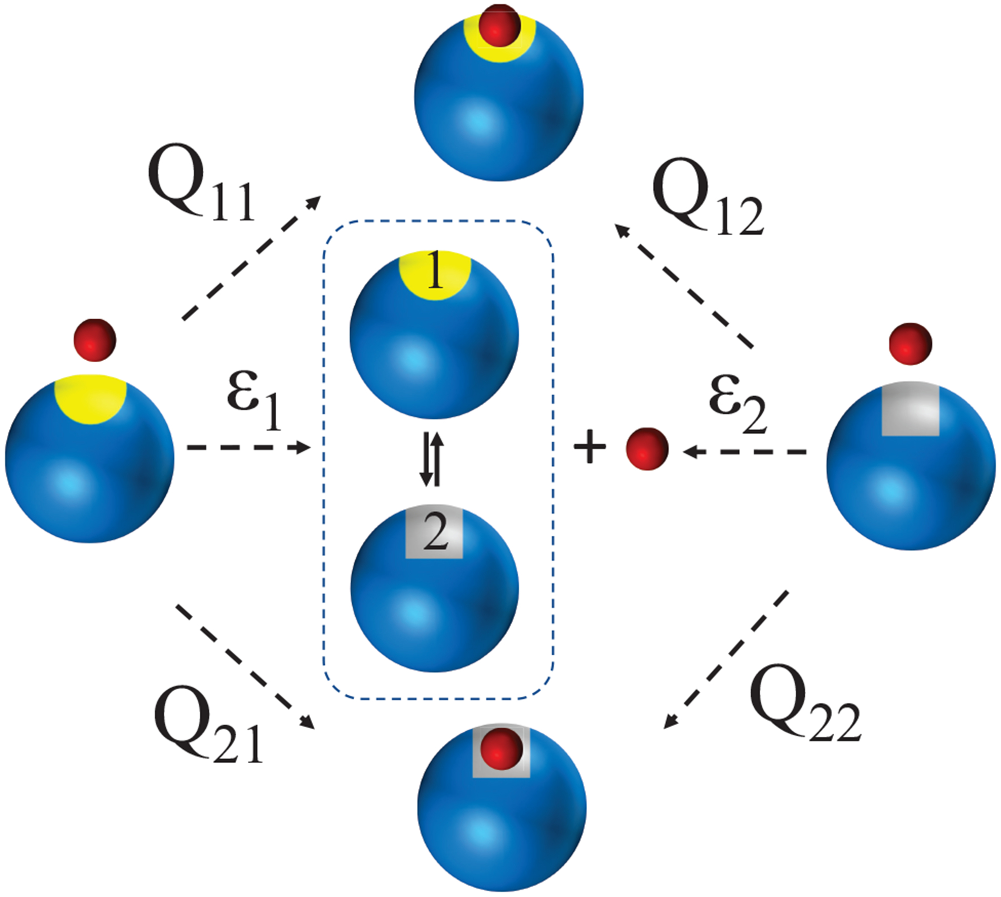
From the definition of the pair association flux in terms of the Green’s function in eqs 3.17, it follows that J_{mnl,m′n′l′(}t)dt is the probability that an X_m − X_n pair irreversibly associates between t and t + dt to form the complex X_l given that initially the system contained an X_m′ − X_n′ pair formed by the dissociation of X_l′ (see Figure 3). In addition, $J_{mnl,m^{\prime }{n}^{\prime }{l}^{\prime }}(t)/{\int }_0^{\infty }{J}_{mnl,m^{\prime }{n}^{\prime }{l}^{\prime }}\left(t^{\prime }\right)d{t}^{\prime }$ is the distribution of times required for the pair X_m − X_n to irreversibly associate to form X_l subject to the same initial condition. Thus J_{mnl,m′n′l′}(t) is the probability density to irreversibly associate, or the association (binding) flux.

Figure 3:

Pair association flux J_{mnl,m′n′l′}(t), which couples bimolecular reactions X_m′+X_n′ ⇌ X_l′ and X_m + X_n ⇌ X_l. A pair of X_m′ (blue ball with yellow round reaction site) and X_n′ (red ball) is formed after dissociation of X_l′ at t = 0. This pair converts into into a pair of X_m (blue ball with gray square reaction site) and X_n (red cube) due to unimolecular transitions X_m′ → X_m and X_n′ → X_n. The X_m − X_n pair associates irreversibly to form X_l. The association flux J_{mnl,m′n′l′}(t) is the probability density that the X_m − X_n pair associates irreversibly at time t to form X_l.

Since $Q_{mnl,m^{\prime }{n}^{\prime }{l}^{\prime }}={\int }_0^{\infty }{J}_{mnl,m^{\prime }{n}^{\prime }{l}^{\prime }}(t)dt$, it follows that Q_{mnl,m′n′l′} is the probability that a pair X_m′ − X_n′ formed immediately after the dissociation of X_l′ will eventually irreversibly react through the X_m + X_n → X_l channel rather than reacting through any other channel or diffusing apart to infinity (i.e., “escape”). Thus the elements of the Q matrix are in fact committors or splitting/capture probabilities.

G. Association fluxes in the framework of the Wilemski-Fixman approximation

To determine the pair fluxes J’s, one must find G_mn,m′n′ by solving eq 3.14 subject to the appropriate initial conditions. This is in general a difficult problem because the “sink” term, R^irr(r) is position-dependent. However, using the Wilemski-Fixman (WF) closure approximation,⁵² it is possible to express the irreversible flux (i.e., the J’s) in terms of the sink-sink correlation functions calculated in the absence of reaction. Specifically, it can be shown that the Laplace transform of J(t), $J(t),\widehat{J}(s)={\int }_0^{\infty }\text{exp}(-st)J(t)dt$, is given by

$$\widehat{\mathit{\text{J}}}\left(s\right)={\left(\mathit{\text{I}}+{\widehat{\mathit{\text{J}}}}^0\left(s\right)\right)}^{-1}{\widehat{\mathit{\text{J}}}}^0\left(s\right)$$ (3.22)

where I is the unit matrix of size N_b and ${\widehat{\mathit{\text{J}}}}^0(s)$ is the Laplace transform of a matrix J⁰(t) with the elements ${\left[J^0(t)\right]}_{\alpha {\alpha }^{\prime }}=J_{mnl,m^{\prime }{n}^{\prime }{l}^{\prime }}^0(t)$ given by

$$J_{mnl,m\prime n\prime l\prime }^0\left(t\right)={\kappa }_{mn\to l}\int {\sigma }_{mnl}\left(\mathit{\text{r}}\right)G_{mn,m\prime n\prime }^0\left(\mathit{\text{r}},t|\mathit{\text{r}}\prime ,0\right){\sigma }_{m\prime n\prime l\prime }\left(\mathit{\text{r}}\prime \right)d\mathit{\text{r}}d\mathit{\text{r}}\prime$$ (3.23)

Here $G_{mn,m^{\prime }{n}^{\prime }}^0$ is the solution of

$$\frac{\partial }{\partial t}{\mathit{\text{G}}}^0\left(\mathit{\text{r}},t\right)={\nabla }^2\left(D{G}^0+G^{0}D\right)+K{G}^0+G^0{K}^{\top }$$ (3.24)

where G⁰ is an N_b × N_b matrix with elements $G_{mn}^0(\mathit{\text{r}},t)$, subject to the same initial condition as G_mn(r, t), $G_{mn}^0\left(t=t^{\prime }\right)=\left({\delta }_{m{m}^{\prime }}{\delta }_{n{n}^{\prime }}+{\delta }_{m{n}^{\prime }}{\delta }_{n{m}^{\prime }}\right)\delta \left(\mathit{\text{r}}-{\mathit{\text{r}}}^{\prime }\right)\left(m^{\prime }\ne n^{\prime }\right)$, where δ(r − r′) is the Dirac delta-function and δ_mn is the Kronecker delta (δ_mn = 1 when m = n and zero otherwise). Thus J⁰(t) is defined just like J(t), but involves the Green’s function in the absence of irreversible association.

In general, to solve eq 3.24, one converts the matrix G⁰ into a vector by applying the “vec” operator (i.e., stacking columns of a matrix into a vector). In this way, eq 3.24 becomes dvec(G⁰)/dt = [∇²(D ⊗ I +I ⊗ D) + (K ⊗ I + I ⊗ K)]vec(G⁰), where ⊗ is the Kronecker product. We have previously used this strategy for the A + B ⇌ C reaction.²³

When all relative diffusion coefficients are the same, it can be shown that

$$J_{mnl,m\prime n\prime l\prime }^0\left(t\right)={\kappa }_{mn\to l}{C}_{mnl,m\prime n\prime l\prime }\left(t\right)\left[{\left(e^{Kt}\right)}_{m{m}^{\prime }}{\left(e^{Kt}\right)}_{n{n}^{\prime }}+{\left(e^{Kt}\right)}_{mn\prime }{\left(e^{Kt}\right)}_{nm\prime }\right]$$ (3.25)

Here C_{mnl,m′n′l′}(t) is the sink-sink correlation function

$$\begin{gathered} C_{mnl,m\prime n\prime l\prime }\left(t\right)=\langle {\sigma }_{mnl}\left(\mathit{\text{r}}\left(t\right)\right){\sigma }_{m\prime n\prime l\prime }\left(\mathit{\text{r}}\left(0\right)\right)\rangle \\ =\int {\sigma }_{mnl}\left(\mathit{\text{r}}\right)g\left(\mathit{\text{r}},t|\mathit{\text{r}}\prime ,0\right){\sigma }_{m\prime n\prime l\prime }\left(\mathit{\text{r}}\prime \right)d\mathit{\text{r}}d\mathit{\text{r}}\prime \end{gathered}$$ (3.26)

where g(r, t|r′, 0) is the free Green’s function, which satisfies ∂g/∂t = D∇²g with the initial condition g(t = 0) = δ(r − r′), subject only to reflecting boundary conditions due to the impenetrability of the molecules. D is the relative diffusion coefficient. This result also assumes that all reacting pairs have the same shape, although different regions can be reactive.

When K = 0, there are no interconversions between the pairs, and eq 3.25 for $J_{mnl,m^{\prime }{n}^{\prime }{l}^{\prime }}^0(t)$ simplifies. The only nonzero flux components are those for m = m′ and n = n′:

$$J_{mnl,mnl\prime }^0\left(t\right)={\kappa }_{mn\to l}{C}_{mnl,mnl\prime }\left(t\right)$$ (3.27)

Thus the first factor in eq 3.25 is $J_{mnl,mn{l}^{\prime }}^0(t)$ in eq 3.27 in the absence of transitions (K = 0). The terms in the square brackets with matrix exponentials correspond to pair conversion X_m′ → X_m and X_n′ → X_n (the first term in the square brackets) and X_m′ → X_n and X_n′ → X_m (the second term in the square brackets). When K = 0, eq 3.27 is formally valid for arbitrary (non-equal) diffusion coefficients.

H. Rate equations in Laplace space

Since eq 3.20 for the time dependence of the concentrations involves a convolution, it simplifies in Laplace space $\left(\widehat{f}(s)={\int }_0^{\infty }f(t)\text{exp}(-st)dt\right)$. In fact, the Laplace transform of eq 3.20 is

$$s\widehat{x}\left(s\right)-x\left(0\right)=S_1\widehat{\mathit{\text{u}}}\left(s\right)+S_2\left(I-\widehat{\mathit{\text{J}}}\left(s\right)\right)\widehat{\mathit{\text{v}}}\left(s\right)$$ (3.28)

where I is the unit matrix of size N_b and x(0) is the vector of initial concentrations.

With the WF approximation for $\widehat{J}(s)$ in eq 3.22, the above equation becomes

$$s\widehat{x}\left(s\right)-x\left(0\right)=S_1\widehat{\mathit{\text{u}}}\left(s\right)+S_2{\left(I+{\widehat{\mathit{\text{J}}}}^0\left(s\right)\right)}^{-1}\widehat{\mathit{\text{v}}}\left(s\right)$$ (3.29)

When all bimolecular reactions are pseudo-first order, this equation can be solved to obtain $\widehat{x}(s)$ explicitly.

I. Extensions of the theory

The above formalism (eqs 3.1, 3.14, and 3.17) with the linearized chemical kinetics matrix K leads to the concentrations that are accurate both at short and long times, but not completely satisfactory at intermediate times when the concentrations are extremely high or when one is close to the irreversible limit. This was shown for A + B ⇌ C when A is static and the B’s are noninteracting point particles that are in excess^11,23 by comparison with the results of accurate many-particle Brownian dynamics simulations.²¹ To increase the accuracy at intermediate times, one can treat the bimolecular reactions of a pair with bulk molecules more accurately. Within the framework of our formalism, this could be done by calculating K using eq 2.5 with the diffusion-influenced rates w, eq 3.19, instead of v. This would result in a time-dependent matrix K and make eq 3.13 difficult to solve. To find a better K that is time-independent, we now replace the chemical rates by the diffusion-influenced rates in the long-time (Markovian) limit.

Consider the case without unimolecular transitions, K₁ = 0. For d[X_i]/dt in the linearized matrix definition, eq 2.5, let us use our Markovian diffusion-influenced rate equations given in eq 3.21. This leads to

$$K_{ij}=\underset{t\to \infty }{\text{lim}}\frac{\partial }{\partial \left[X_j\right]}{\left(S_2\left(\mathit{\text{I}}-\mathit{\text{Q}}\left(\mathit{\text{K}}\right)\right)\mathit{\text{v}}\right)}_i$$ (3.30)

where we have explicitly indicated that Q depends on the matrix K. The derivative is taken with respect to concentrations [X_j], which enter v (not Q). Since the elements of K appear on both sides of eq 3.30, this equation must be solved self-consistently. This is the generalization of our self-consistent relaxation time approximation applied to A + B ⇌ C²³ where it leads to significant improvement at intermediate times.

If we would solve eq 3.30 iteratively, the simplest procedure would be to set K = 0 on the right hand side, i.e., replace Q(K) by Q(K = 0) ≡ Q(0). For A + B ⇌ C, this amounts to replacing the intrinsic chemical rate constants in K by their diffusion-influenced counterparts.

What do we do when unimolecular processes are also present? The same question was raised in a study²⁸ of the kinetics of A + B ⇌ C in the presence of unimolecular decay of A and C. The best agreement with numerical simulations was found when the effective rate constants were determined in the absence of unimolecular reactions. Then the unimolecular rate constants were added to get a new and final K, which was used to calculate the concentrations. This strategy is reasonable because one does not expect the unimolecular rates to be modified and so we recommend it in general.

IV. Reversible binding to a single site

The goal of the rest of this paper is to illustrate how the general formalism can be applied to specific cases. We begin with the simplest bimolecular reaction where A and B can bind reversibly to form C (see Figure 4(a)):

$$A+B\underset{{\kappa }_d}{\overset{{\kappa }_a}{\rightleftharpoons }}C$$ (4.1)

where κ_a ≡ κ_AB→C and κ_d ≡ κ_C→AB are the intrinsic (chemical) association and dissociation rate constants. We have considered this case in some detail previously²³ assuming isotropic contact reactivity. Here it will be shown that these results are also valid for non-local anisotropic reactivity within the framework of the WF approximation.

Figure 4:

Single-site reversible binding A+B ⇌ C when the B’s are in excess. (a) A ligand B (red) binds reversibly to a macromolecule A (blue) with one binding site (yellow) to form a complex C. (b) For low concentrations (K = 0), the solution of the many-body problem is reduced to a pair problem involving a single A and a single B that can associate irreversibly to form C. (c) In the case of large ligand concentration, the A − B pair becomes coupled with the C − B pair because an A can bind a ligand from the bulk (red dashed ball) to form C. Thus a reactive A − B pair interconverts with an unreactive C − B pair.

A. Chemical kinetics rate equations

Reversible binding to a single site has one reaction channel. Let X₁ = A, X₂ = B, X₃ = C.

Then the net reaction rate in eq 2.2 is

$$v\left(t\right)\equiv v_{123}\left(t\right)\equiv v_{ABC}\left(t\right)={\kappa }_a\left[A\left(t\right)\right]\left[B\left(t\right)\right]-{\kappa }_d\left[C\left(t\right)\right]$$ (4.2)

The equilibrium concentrations satisfy the detailed balance condition, κ_aA_eqB_eq = κ_dC_eq, so the reaction rate vanishes at equilibrium, v = 0.

The rate equations, eq 2.3, can be written as

$$\frac{dx}{dt}=\frac{d}{dt}\left(\begin{array}{l}\left[A\left(t\right)\right]\hfill \\ \left[B\left(t\right)\right]\hfill \\ \left[C\left(t\right)\right]\hfill \end{array}\right)=S_{2}v\left(t\right)\equiv \left(\begin{array}{c}-1\\ -1\\ 1\end{array}\right)v\left(t\right)$$ (4.3)

Since there are three species and one reaction channel, the stoichiometric matrix S₂ in eq 4.3 is just one column with three elements (−1, −1, 1).

The linearized matrix K, eq 2.5, that describes the relaxation of the system to equilibrium is:

$$K=\left(\begin{array}{ccc}-{\kappa }_a{B}_{eq}& -{\kappa }_a{A}_{eq}& {\kappa }_d\\ -{\kappa }_a{B}_{eq}& -{\kappa }_a{A}_{eq}& {\kappa }_d\\ {\kappa }_a{B}_{eq}& {\kappa }_a{A}_{eq}& -{\kappa }_d\end{array}\right)$$ (4.4)

This matrix has two zero eigenvalues and one nonzero eigenvalue −k₀, where k₀ = κ_a(A_eq + B_eq) + κ_d. Thus the system approaches equilibrium as exp(−k₀t).

B. Diffusion-modified rate equations

The influence of diffusion on the kinetics is accounted for by replacing the chemical reaction rate v(t) by its diffusion-influenced counterpart (see eq 3.1):

$$\frac{dx}{dt}=\frac{d}{dt}\left(\begin{array}{l}\left[A\left(t\right)\right]\hfill \\ \left[B\left(t\right)\right]\hfill \\ \left[C\left(t\right)\right]\hfill \end{array}\right)=\left(\begin{array}{c}-1\\ -1\\ 1\end{array}\right)\left(v\left(t\right)-J\left(t\right)*v\left(t\right)\right)$$ (4.5)

where $J(t)*v(t)={\int }_0^{t}J(t-\tau )v(\tau )d\tau$. The irreversible flux J(t) ≡ J_ABC,ABC(t) is given by (see eq 3.17):

$$J\left(t\right)={\kappa }_a\int \sigma \left(\mathit{\text{r}}\right)G_{AB,AB}\left(\mathit{\text{r}},t|\mathit{\text{r}}\prime ,0\right)\sigma \left(\mathit{\text{r}}\prime \right)d\mathit{\text{r}}d\mathit{\text{r}}\prime$$ (4.6)

where σ(r) ≡ σ_ABC(r) is the sink function, which is localized in the reagion of conformational space where reaction occurs. G_AB,AB(r, t | r′, 0) describes the evolution of the A − B pair that can irreversibly bind. It can be obtained by solving eq 3.14 subject to the appropriate boundary conditions.

In the Markovian limit, eq 4.5 becomes (see eqs 3.2–3.3)

$$\frac{dx}{dt}=\frac{d}{dt}\left(\begin{array}{l}\left[A\left(t\right)\right]\hfill \\ \left[B\left(t\right)\right]\hfill \\ \left[C\left(t\right)\right]\hfill \end{array}\right)=\left(\begin{array}{c}-1\\ -1\\ 1\end{array}\right)\left(1-Q\right)v\left(t\right)$$ (4.7)

where $Q={\int }_0^{\infty }J(t)dt$. Equation 4.7 implies that, in the Markovian limit, the diffusion-influenced rate equations are the same as the chemical ones but with “renormalized” rate coefficient, i.e., κ_a and κ_d are replaced by κ_a(1 − Q) and κ_d(1 − Q), respectively. Thus, in this limit, the diffusion-modified kinetic scheme is

$$A+B\underset{{\kappa }_d\left(1-Q\right)}{\overset{{\kappa }_a\left(1-Q\right)}{\rightleftharpoons }}C$$ (4.8)

Note that both intrinsic rates are scaled by the same factor, so that the equilibrium constant is unaffected by diffusion.

C. Association flux J(t) for an isolated pair

The simplest version of our theory is obtained when the concentrations are sufficiently small so that reactions of an A − B pair with molecules in the bulk can be ignored. In this case, the linearized matrix in eq 3.14 that describes the reaction with bulk molecules can be set to zero, K = 0. Then the A − B pair is not coupled with any other pair, and G_AB,AB(r, t | r′, 0) ≡ G(r, t | r′, 0) satisfies

$$\frac{\partial }{\partial t}G=D{\nabla }^{2}G-{\kappa }_a\sigma \left(\mathit{\text{r}}\right)G$$ (4.9)

where D = D_A +D_B is the relative diffusion coefficient. Initially, G(t = 0) = δ(r − r′). This equation describes the evolution of an isolated pair that can either irreversibly associate or diffuse apart (see Figure 4(b)).

We now show that the pair association flux J(t) obtained by using G in eq 4.9 is related to the survival probability S(t) of an A − B pair initially located in the reaction region (more precisely, the initial separation between A and B is drawn from the probability density σ(r)). This survival probability is defined as $S(t)=\int G\left(\mathit{\text{r}},t|{\mathit{\text{r}}}^{\prime },0\right)\sigma \left({\mathit{\text{r}}}^{\prime }\right)d\mathit{\text{r}}d{\mathit{\text{r}}}^{\prime }$, i.e., the probability that an A − B pair survives at time t given that the initial distribution of the relative coordinate was σ(r′). Multiplying both sides of eq 4.9 by σ(r′), integrating both sides with respect to r and r′, and using the fact that the integral involving the Laplacian vanishes, it follows that dS/dt = −J(t), or

$$J\left(t\right)=-\frac{dS\left(t\right)}{dt}$$ (4.10)

This relation means that J(t) is the probability density that an A − B pair, initially in the reactive region, irreversibly binds at time t (see Figure 5(a)).

Figure 5:

Association flux J(t) for single-site binding. (a) An A − B pair is formed by the dissociation of C at t = 0, so that initially the ligand (red ball) is located near the binding site (yellow) of the macromolecule (blue ball). The pair can diffuse apart or irreversibly bind at time t with probability density J(t). (b) At higher ligand concentrations, one must consider the possibility that an A − B pair can be converted to a C − B pair because the A can bind a ligand from the bulk (dashed red ball). The C − B pair changes into the A − B pair when C dissociates.

The above relation implies that $Q={\int }_0^{\infty }J(t)dt$ (which enters the Markovian rate equation, eq 4.7) has a simple physical interpretation. Using eq 4.10 in the definition of Q, we have $Q=-{\int }_0^{\infty }(dS/dt)dt=S(0)-S(\infty )=1-S(\infty )$. Here S(∞) ≡ ε is the survival probability of the pair at long times, or, equivalently, the probability that a pair diffused apart (“escaped”). Thus Q is the probability that an A − B pair, initially in the reactive region, eventually irreversibly reacted (“captured”) rather than diffused apart. The capture and escape probabilities are illustrated in Figure 6.

Figure 6:

Capture and escape probabilities for single-site binding. An A and B pair located initially in the reaction site eventually either bind with probability Q or escape with probability ε = 1 − Q.

Within the framework of the WF approximation, the Laplace transform of J(t) is given by (see eq 3.22)

$$\widehat{J}\left(s\right)=\frac{{\widehat{J}}^0\left(s\right)}{1+{\widehat{J}}^0\left(s\right)}$$ (4.11)

When K = 0, $K=0,{\widehat{J}}^0(s)$ is the Laplace transform of J⁰(t) given by (see eq 3.27)

$$J^0\left(t\right)={\kappa }_{a}C\left(t\right)$$ (4.12)

where C(t) ≡ C_ABC,ABC(t) is the sink-sink correlation function:

$$C\left(t\right)=\int \sigma \left(\mathit{\text{r}}\right)g\left(\mathit{\text{r}},t|\mathit{\text{r}}\prime ,0\right)\sigma \left(\mathit{\text{r}}\prime \right)d\mathit{\text{r}}d\mathit{\text{r}}\prime$$ (4.13)

Here g(r, t | r′, 0) is the Green’s function in the absence of reaction. Thus, when K = 0,

$$\widehat{J}\left(s\right)=\frac{{\kappa }_a\widehat{C}\left(s\right)}{1+{\kappa }_a\widehat{C}\left(s\right)}$$ (4.14)

Relation to the Smoluchowski rate coefficient

It turns out that, within the WF approximation, the Laplace transform of the time-dependent Smoluchowski rate coefficient, k_irr(t), that describes the irreversible reaction A + B → C is given by^53,54

$$\frac{1}{s{\widehat{k}}_{irr}\left(s\right)}=\frac{1}{{\kappa }_a}+\widehat{C}\left(s\right)$$ (4.15)

Therefore, $\widehat{J}\left(s\right)$ and ${\widehat{k}}_{irr}\left(s\right)$ are related. It can be shown using eqs 4.14 and 4.15 that in the time domain

$${\kappa }_{a}J\left(t\right)=-\frac{d}{dt}{k}_{irr}\left(t\right)$$ (4.16)

where we used the fact that k_irr(0) = κ_a. By letting κ_a → ∞ in eq 4.15, it can be seen that $1/s\widehat{C}(s)$ is the Laplace transform of the irreversible rate coefficient in the diffusion-control limit.

The importance of these relations is that one can find $\widehat{C}$ and hence $\widehat{J}$ by exploiting the existing literature, where ${\widehat{k}}_{irr}$ has been calculated for various models of anisotropic reactivity,^55–62 including those within the framework of the WF approximation⁵² or the equivalent⁵³ “constant flux approximation”.⁶³

For the simplest case of isotropic contact reactivity at distance R described by the sink term σ(r) = δ(r − R)/4πR² (which is equivalent⁶⁴ to the Collins-Kimball partially absorbing boundary condition⁶⁵), one has

$$\frac{1}{s{\widehat{k}}_{irr}\left(s\right)}=\frac{1}{{\kappa }_a}+\frac{1}{4\pi DR\left(1+\sqrt{s{R}^2/D}\right)}$$ (4.17)

so that

$$\widehat{C}\left(s\right)=\frac{1}{4\pi DR\left(1+\sqrt{s{R}^2/D}\right)}$$ (4.18)

Note that $\widehat{C}\left(0\right)={\int }_0^{\infty }C\left(t\right)dt$ is the reciprocal of the Smoluchowski diffusion-controlled rate coefficient, 4πDR.

D. Association flux J(t) in general

We now turn to the case where K ≡ 0 due to reactions of a pair with bulk molecules. Within the WF approximation, $\widehat{J}\left(s\right)$ in terms of ${\widehat{J}}^0\left(s\right)$ is still given by eq 4.11. However, to find ${\widehat{J}}^0\left(s\right)$, eq 3.23, one has to solve the matrix equation, eq 3.24. To calculate ${\widehat{J}}^0\left(s\right)$ for arbitrary diffusion coefficients, one would first have to vectorize the matrix equation and proceed as we have outlined previously.²³ When all the relative diffusion coefficients are the same, we can use eq 3.25 with m = m′ = 1 = A, n = n′ = 2 = B, l = l′ = 3 = C

$$J^0\left(t\right)={\kappa }_{a}C\left(t\right)\left[{\left(e^{\mathit{\text{K}}t}\right)}_{AA}{\left(e^{\mathit{\text{K}}t}\right)}_{BB}+{\left(e^{\mathit{\text{K}}t}\right)}_{AB}{\left(e^{\mathit{\text{K}}t}\right)}_{BA}\right]$$ (4.19)

where C(t) is the sink-sink correlation function, eq 4.13, and K is the linearized matrix given in eq 4.4. The factor κ_aC(t) is J⁰(t) for an isolated pair, eq 4.12. The terms with matrix exponentials accounts for the reaction with bulk molecules. The term (exp(Kt))_AA(exp(Kt))_BB corresponds to an A − B pair, where A remains A and B remains B at time t. The term (exp(Kt))_AB(exp(Kt))_BA corresponds to an A − B pair, in which an A molecule at t = 0 becomes B at time t while B becomes A.

To evaluate the matrix exponentials, we use the identity for K in eq 4.4

$$e^{\mathit{\text{K}}t}=\mathit{\text{I}}+\mathit{\text{K}}\left(1-e^{-k_{0}t}\right)/k_0$$ (4.20)

where I is a 3 × 3 unit matrix and k₀ = κ_a(A_eq + B_eq) + κ_d. Using this we find that eq 4.19 reduces to

$$J^0\left(t\right)/{\kappa }_a=C\left(t\right)\left(\mu +2\nu +\left(1-\mu -4\nu \right)e^{-k_{0}t}+2\nu e^{-2k_{0}t}\right)$$ (4.21)

where μ = k_d/k₀, $\nu ={\kappa }_a^2{A}_{eq}{B}_{eq}/k_0^2$. In Laplace space, this becomes

$${\widehat{J}}^0\left(s\right)/{\kappa }_a=\left(\mu +2\nu \right)\widehat{C}\left(s\right)+\left(1-\mu -4\nu \right)\widehat{C}\left(s+k_0\right)+2\nu \widehat{C}\left(s+2k_0\right)$$ (4.22)

where $\widehat{C}\left(s\right)$ is the Laplace transform of C(t). When $\widehat{C}\left(s\right)$ is eliminated in favor of ${\widehat{k}}_{irr}(s)$ using eq 4.15, this becomes eq 6.12 of our previous paper²³ if we identify $1/s{\widehat{k}}_{SG}(s)$ with $\left(1+{\widehat{J}}^0(s)\right)/{\kappa }_a$. Thus our previous results²³ that were derived for isotropic contact reactivity, are actually valid for anisotropic reactivity within the framework of the WF approximation.

In the low concentration limit (A_eq → 0, B_eq → 0), J⁰(t) in eq 4.21 reduces to the result given in eq 4.12. Another interesting limit is the pseudo-first order one where the concentration of B is so large (compared to that of A) that it does not change in time. The corresponding J⁰(t) is obtained from eq 4.21 by letting A_eq → 0 and B_eq → [B]. In this way we find that

$$J^0\left(t\right)={\kappa }_{a}C\left(t\right)\left(\mu +\left(1-\mu \right)e^{-k_{0}t}\right)$$ (4.23)

where now μ = κ_d/(κ_a[B]+κ_d), k₀ = κ_a[B]+κ_d. The resulting association flux J(t), just like the one in the low concentration limit, has a simple physical interpretation (see Figure 5(b)). It is the negative of the derivative of the survival probability, S(t), of an A − B pair starting out in the reaction region (i.e., as if it was just formed by the dissociation of C) that can now interconvert with an unreactive C − B pair but still bind irreversibly or diffuse apart. The interconversion between the reactive or “open” (A − B) and unreactive or “closed” (C-B) pairs is described by forward, κ_a[B], and reverse, κ_d, rate constants. This is a form of “stochastic gating”^66–68 and in fact J(t) in eqs 4.11 and 4.23 is related to the time derivative of the stochastically-gated irreversible diffusion coefficient.³⁶

This theory (eqs 4.5, 4.11, and 4.22) is exact at short and long times and in the geminate limit, but as discussed before, it can be extended to improve its accuracy at intermediate times for high concentrations. This is done by replacing the linearized matrix K, eq 4.4 by the self-consistent solution of eq 3.30. Since here there is only one reaction channel, Q(K) in eq 3.30 is actually a number and the new K can be obtained from eq 4.4 by replacing the intrinsic rate constants κ_a and κ_d by k_a = κ_a(1 − Q) and k_d = κ_d(1 − Q). Here, according to eq 4.11, $1-Q=1-\widehat{J}(0)={\left(1+{\widehat{J}}^0(0)\right)}^{-1}$ and ${\widehat{J}}^0(0)$ is found by Laplace transforming eq 4.23 with k₀ replaced by k_a[B] + k_d. The rate constants k_a and k_d in k₀ are then found self-consistently. Since we have previously described²³ this procedure in the present context in some detail, we do not elaborate on it here.

E. Long-time asymptotics

The relaxation function $\mathcal{R}(t)$ is defined as the normalized deviation from equilibrium:

$$\mathcal{R}\left(t\right)=\frac{\left[A\left(t\right)\right]-A_{eq}}{\left[A\left(0\right)\right]-A_{eq}}=\frac{\left[B\left(t\right)\right]-B_{eq}}{\left[B\left(0\right)\right]-B_{eq}}=\frac{\left[C\left(t\right)\right]-C_{eq}}{\left[C\left(0\right)\right]-C_{eq}}$$ (4.24)

so that $\mathcal{R}\left(0\right)=1$ and $\mathcal{R}\left(\infty \right)=0$. The relaxation function is the same for all species, as follows from the mass conservation, and thus completely determines the kinetics for arbitrary initial concentrations.

When the chemical kinetics rate equations, eq 4.3, are linearized about equilibrium, the relaxation function is a single-exponential, $\mathcal{R}(t)=\text{exp}\left(-k_{0}t\right)$, where k₀ = κ_a(A_eq +B_eq)+κ_d. In the presence of diffusion, the relaxation function of a reversible reaction becomes a power-law asymptotically (i.e., at very long times).^49,50,69 By linearizing the diffusion-influenced rate equations, eq 4.5, the Laplace transform of the relaxation function can be shown to be

$$\widehat{\mathcal{R}}\left(s\right)={\left(s+\frac{k_0}{1+{\widehat{J}}^0\left(s\right)}\right)}^{-1}$$ (4.25)

where we have used eq 4.11.

To find $\mathcal{R}\left(t\right)$ as t → ∞, we consider the s → 0 limit of $\widehat{\mathcal{R}}(s)$. In this limit, $\widehat{\mathcal{R}}(s)\to {\widehat{J}}^0(s)/k_0$ and so $\mathcal{R}(t)\to J_0(t)/k_0$. Using eq 4.21 for J⁰(t), it can be seen that only the first term survives at long times, so that $\mathcal{R}(t)\to (\mu +2\nu ){\kappa }_{a}C(t)/k_0$. Now C(t) in eq 4.13 is (4πDt)^−3/2 as t → ∞ since g(r, t j r′, 0) → (4πDt)^−3/2 at long times and ∫ σ(r)dr = 1. In this way we find

$$\mathcal{R}\left(t\right)~\left(\frac{K_{eq}}{{\left(1+K_{eq}\left(A_{eq}+B_{eq}\right)\right)}^2}+\frac{2K_{eq}^3{A}_{eq}{B}_{eq}}{{\left(1+K_{eq}\left(A_{eq}+B_{eq}\right)\right)}^3}\right){\left(4\pi D_{AB}t\right)}^{-3/2}$$ (4.26)

where K_eq = κ_a/κ_d is the equilibrium constant. This is identical to the exact result we derived previously²⁴ starting with the master equation for reactants hopping on a lattice and using the Poisson representation⁵¹ to obtain the corresponding formally exact Langevin equation.

V. Reversible binding to two sites

Consider a macromolecule, A, with two inequivalent sites that can bind a ligand, B, to form two different complexes, C₁ and C₂ (see Figure 7(a)). The corresponding kinetic scheme is

$$C_1\underset{{\kappa }_{a1}}{\overset{{\kappa }_{d1}}{\rightleftharpoons }}A+B\underset{{\kappa }_{d2}}{\overset{{\kappa }_{a2}}{\rightleftharpoons }}{C}_2$$ (5.1)

where the intrinsic association and dissociation rate constants are ${\kappa }_{ai}={\kappa }_{AB\to C_i}$ and ${\kappa }_{di}={\kappa }_{C_i\to AB}$, i = 1,2. For the sake of simplicity, we consider the model where only one ligand can bind to the molecule, so the unoccupied sites in C₁ and C₂ are unreactive. This scheme can also describe protein-protein association and even double phosphorylation, where a substrate S₀ can be phosphorylated by an enzyme E to form singly (S₁) and doubly (S₂) modified substrates. Specifically, if C₁ = S₀E, C₂ = S₁E, A = S₁, B = E, κ_a1 = 0, κ_d1 = κ_c0 (the catalytic rate), then the above scheme is the central fragment of

$$S_0+E\underset{{\kappa }_{d0}}{\overset{{\kappa }_{a0}}{\rightleftharpoons }}{S}_{0}E\stackrel{{\kappa }_{c0}}{\to }{S}_1+E\underset{{\kappa }_{d1}}{\overset{{\kappa }_{a1}}{\rightleftharpoons }}{S}_{1}E\stackrel{{\kappa }_{c1}}{\to }{S}_2+E$$ (5.2)

It was shown previously^33,37 that diffusion can dramatically modify this scheme by changing the above distributive mechanism into a processive one.

Figure 7:

Two-site reversible binding C₁ ⇌ A + B ⇌ C₂. (a) A ligand B (red) reversibly binds to a macromolecule A with two binding sites to form C₁ (first site, yellow) or C₂ (second site, gray). (b) For low concentrations, the many-body problem is reduced to a pair problem involving an A and a B that can bind irreversibly at either site to form C₁ or C₂.

A. Chemical kinetics rate equations

Since there are two reaction channels, there are two net rates. Let X₁ = A, X₂ = B, X₃ = C₁, X₄ = C₂. Then the reaction rates in eq 2.2 are

$$\begin{gathered} v_1\left(t\right)\equiv v_{123}(t)\equiv v_{AB{C}_1}\left(t\right)={\kappa }_{a1}\left[A\left(t\right)\right]\left[B\left(t\right)\right]-{\kappa }_{d1}\left[C_1\left(t\right)\right] \\ {v}_2\left(t\right)\equiv v_{124}(t)\equiv v_{AB{C}_4}\left(t\right)={\kappa }_{a2}\left[A\left(t\right)\right]\left[B\left(t\right)\right]-{\kappa }_{d2}\left[C_2\left(t\right)\right] \end{gathered}$$ (5.3)

The chemical kinetics rate equations can be written as

$$\frac{\mathit{\text{d}}x}{dt}=\frac{d}{dt}\left(\begin{array}{c}\left[A\left(t\right)\right]\\ \left[B\left(t\right)\right]\\ \left[C_1\left(t\right)\right]\\ \left[C_2\left(t\right)\right]\end{array}\right)=S_2\mathit{\text{v}}\left(t\right)=\left(\begin{array}{cc}-1& -1\\ -1& -1\\ 1& 0\\ 0& 1\end{array}\right)\cdot \left(\begin{array}{c}{v}_1\left(t\right)\\ v_2\left(t\right)\end{array}\right)$$ (5.4)

The linearized matrix K obtained from eq 2.5 is a 4 × 4 matrix. It has two zero and two non-zero eigenvalues, which can be found by solving a quadratic equation.

B. Diffusion-modified rate equations

The influence of diffusion on the kinetics can be described by replacing the rates of conventional chemical kinetics by their diffusion-influenced counterparts (see eq 3.1):

$$\frac{d}{dt}\left(\begin{array}{c}\left[A\left(t\right)\right]\\ \left[B\left(t\right)\right]\\ \left[C_1\left(t\right)\right]\\ \left[C_2\left(t\right)\right]\end{array}\right)=\left(\begin{array}{cc}-1& -1\\ -1& -1\\ 1& 0\\ 0& 1\end{array}\right)\cdot \left(\begin{array}{l}{v}_1\left(t\right)-J_{11}\left(t\right)*v_1\left(t\right)-J_{12}\left(t\right)*v_2\left(t\right)\hfill \\ v_2\left(t\right)-J_{21}\left(t\right)*v_1\left(t\right)-J_{22}\left(t\right)*v_2\left(t\right)\hfill \end{array}\right)$$ (5.5)

where we use * to denote the time convolution $f(t)*g(t)\equiv {\int }_0^{t}f\left(t-t^{\prime }\right)g\left(t^{\prime }\right)d{t}^{\prime }$. Here the matrix of pair association fluxes, J, has four components $J_{ij}(t)\equiv J_{AB{C}_i,AB{C}_j}(t)$ (the indexes i, j = 1, 2 refer to the first or second reaction channel), which are given by (see eq 3.17)

$$J_{ij}\left(t\right)={\kappa }_{ai}\int {\sigma }_i\left(\mathit{\text{r}}\right)G_{AB,AB}\left(\mathit{\text{r}},t|\mathit{\text{r}}\prime ,0\right){\sigma }_j\left(\mathit{\text{r}}\prime \right)d\mathit{\text{r}}d\mathit{\text{r}}\prime$$ (5.6)

where ${\sigma }_i(\mathit{\text{r}})\equiv {\sigma }_{AB{C}_i}(\mathit{\text{r}})$ differs from zero around the binding site of the channel A+B ⇌ C_i and G_AB,AB describes the evolution of the A − B pair that can eventually irreversibly react. Not all J’s are independent because of detailed balance. It follows from eq 3.18 by setting m = 1, n = 2, l = 3 and m′ = 1, n′ = 2, l′ = 4 that

$$J_{12}\left(t\right){\kappa }_{a2}=J_{21}\left(t\right){\kappa }_{a1}$$ (5.7)

It can be seen that in this formulation diffusion simply couples the two chemical reaction rates.

In the Markovian limit, eq 5.5 becomes

$$\frac{d}{dt}\left(\begin{array}{c}\left[A\left(t\right)\right]\\ \left[B\left(t\right)\right]\\ \left[C_1\left(t\right)\right]\\ \left[C_2\left(t\right)\right]\end{array}\right)=\left(\begin{array}{cc}-1& -1\\ -1& -1\\ 1& 0\\ 0& 1\end{array}\right)\cdot \left(\begin{array}{l}\left(1-Q_{11}\right)v_1\left(t\right)-Q_{12}{v}_2\left(t\right)\hfill \\ \left(1-Q_{22}\right)v_2\left(t\right)-Q_{21}{v}_1\left(t\right)\hfill \end{array}\right)$$ (5.8)

As follows from eq 5.7, Q₂₁κ_a1 = Q₁₂κ_a2.

Because the reaction rates v₁(t) and v₂(t) are coupled, the above Markovian diffusion-influenced rate equation does not have the same structure as the usual chemical kinetics ones. Therefore, one cannot simply rescale or renormalize the intrinsic rate constants as in the single-site case. In order to cast eq 5.8 into standard form, let us write the diffusion-influenced rates as follows

$$\left(1-Q_{11}\right)v_1\left(t\right)-Q_{12}{v}_2\left(t\right)={\epsilon }_1{v}_1\left(t\right)-u\left(t\right)$$

$$\left(1-Q_{22}\right)v_2\left(t\right)-Q_{21}{v}_1\left(t\right)\equiv {\epsilon }_2{v}_2\left(t\right)+u\left(t\right)$$ (5.9)

where we have defined the escape probabilities εi as

$${\epsilon }_1=1-Q_{11}-Q_{21}$$

$${\epsilon }_2=1-Q_{22}-Q_{12}$$ (5.10)

and the unimolecular reaction rate as

$$u\left(t\right)\equiv Q_{12}{v}_2\left(t\right)-Q_{21}{v}_1\left(t\right)=Q_{21}{\kappa }_{d1}\left[C_1\right]-Q_{12}{\kappa }_{d2}\left[C_2\right]$$ (5.11)

To get the last equality, we used the v’s in eq 5.3 and the detailed balance condition Q₂₁κ_a1 = Q₁₂κ₂. The net rate u(t) corresponds to a new unimolecular reaction channel C₁ ⇌ C₂ with rate constants ${\kappa }_{C_1\to C_2}={\kappa }_{d1}{Q}_{21}$ and ${\kappa }_{C_2\to C_1}={\kappa }_{d2}{Q}_{12}$.

We are now in a position to rewrite eq 5.8 in a standard form:

$$\frac{d}{dt}\left(\begin{array}{c}\left[A\left(t\right)\right]\\ \left[B\left(t\right)\right]\\ \left[C_1\left(t\right)\right]\\ \left[C_2\left(t\right)\right]\end{array}\right)=\left(\begin{array}{c}0\\ 0\\ -1\\ 1\end{array}\right)u\left(t\right)+\left(\begin{array}{cc}-1& -1\\ -1& -1\\ 1& 0\\ 0& 1\end{array}\right)\cdot \left(\begin{array}{c}{\epsilon }_1{v}_1\left(t\right)\\ {\epsilon }_2{v}_2\left(t\right)\end{array}\right)$$ (5.12)

Comparing this to the original chemical kinetics result in eq 5.4, we see that not only did we have to rescale the reaction rates by ε₁ and ε₂ , but we had to introduce a new unimolecular reaction channel that allows C₁ and C₂ to directly interconvert. The physical reason why a new channel appears is illustrated in Figure 1(b). The ligand that just dissociated from one site can rebind at the other rather than diffuse away into the bulk. The probability of this process approaches zero as diffusion becomes very fast (i.e., in the reaction controlled limit).

The new diffusion-influenced rate equations, eq 5.12, correspond to the following kinetic scheme:

$$C_1\underset{{\kappa }_{a1}{\epsilon }_1}{\overset{{\kappa }_{d1}{\epsilon }_1}{\rightleftharpoons }}A+B\underset{{\kappa }_{d2}{\epsilon }_1}{\overset{{\kappa }_{a2}{\epsilon }_1}{\rightleftharpoons }}{C}_2$$

$$C_1\underset{{\kappa }_{d2}{Q}_{12}}{\overset{{\kappa }_{d1}{Q}_{21}}{\rightleftharpoons }}{C}_2$$ (5.13)

Comparing this to the conventional kinetic scheme in eq 5.1, we see that the intrinsic association and dissociation rate constants have been multiplied by the corresponding escape probabilities. In addition, a new reaction channel appears connecting the two complexes C₁ and C₂. The rate constants of the new channel have a simple physical interpretation. For example, the rate constant of the transition C₁ → C₂ is the product of the dissociation rate constant of C₁ (κ_d1) and the probability (Q₂₁) that the A − B pair, generated immediately after the dissociation of C₁, reacts by binding at the second site to form C₂ rather than diffusing apart or rebinding to the first site. Finally note that this new diffusion-modified scheme is cyclic, but the product of the rate constants in one direction is the same as in the other as a result of the detailed balance condition κ_a1Q₂₁ = κ_a2Q₁₂.

We have previously found^33,35 that, for multisite phosphorylation, the simplest kinetic scheme that accounts for diffusion cannot be obtained just by rescaling the intrinsic rates, but a new reaction channel must be introduced. The physical reason for this is that a kinase, after phosphorylating one site, can rebind to another site and modify it before diffusing away. An interesting consequence of this effect is that changing the magnitude of the diffusion constant can change the mechanism of phosphorilation.³⁷ Specifically, the mechanism that is distributive in the reaction-controlled limit can become processive in the diffusion-controlled limit.

C. Association fluxes J(t) and committors Q

We shall find the association fluxes J_ij(t) only in the low concentration limit (K = 0) because interesting coupling between the reaction channels already happens in this case. When K = 0, the A − B pair is not coupled to any other pair and G_AB,AB(r, t j r′, 0) ≡ G(r, t j r′, 0) in eq 5.6 satisfies (see eq 3.14 with K = 0):

$$\frac{\partial }{\partial t}G=D{\nabla }^{2}G-\left({\kappa }_{a1}{\sigma }_1\left(\mathit{\text{r}}\right)+{\kappa }_{a2}{\sigma }_2\left(\mathit{\text{r}}\right)\right)G$$ (5.14)

with G(t = 0) = δ(r − r′). This equation describes the evolution of an isolated pair that can irreversibly bind at the first or second reaction site or diffuse apart (see Figure 7(b)).

In complete analogy to the single-site case, the J’s have a simple physical interpretation. Specifically, J_ij(t) is the probability density that an A − B pair, initially located in reaction region j, binds at site i at time t. Consequently, $Q_{ij}={\int }_0^{\infty }{J}_{ij}(t)dt$ that enter the Markovain diffusion-influenced rate equations, eq 5.8, also have simple physical interpretations, as shown in Figure 8. Specifically, Q_ij is the probability that an A − B pair initially located in reaction site j will eventually irreversibly bind at site i rather than diffuse apart or bind at the other site. The coefficients ε_i that enter the diffusion-modified kinetic scheme in eq 5.13 are the escape probabilities. For example, ε₁ is the probability that a pair A − B initially located in the first reaction site eventually diffuses apart rather than irreversibly binds.

Figure 8:

Capture and escape probabilities for two-site binding. A (blue) and B (red) located initially near the first (yellow, left) reaction site will eventually bind to the first site with probability Q₁₁ or to the second site Q₂₁ or escape with probability ε₁ = 1 − Q₁₁ − Q₂₁. A and B located initially near the second (gray, right) site eventually bind to the first site with probability Q₁₂ or to the second site Q₂₂ or escape with probability ε₂ = 1 − Q₁₂ − Q₂₂.

Within the WF approximation, the Laplace transform of the 2 × 2 matrix J(t) is given as before by (see eq 3.22)

$$\widehat{\mathit{\text{J}}}\left(s\right)={\left(\mathit{\text{I}}+{\widehat{\mathit{\text{J}}}}^0\left(s\right)\right)}^{-1}{\widehat{\mathit{\text{J}}}}^0\left(s\right)$$ (5.15)

where I is a 2 × 2 unit matrix.

When K = 0, the matrix elements ${\widehat{J}}_{ij}^0\left(s\right)\equiv {\widehat{J}}_{AB{C}_i,AB{C}_j}^0\left(s\right)$ are (see eq 3.27)

$${\widehat{J}}_{ij}^0\left(s\right)={\kappa }_{ai}{\widehat{C}}_{ij}\left(s\right)$$ (5.16)

where ${\widehat{C}}_{ij}\left(s\right)$ is the Laplace transform of the sink-sink auto- and cross-correlation functions (see eq 3.26):

$$C_{ij}\left(t\right)=\int {\sigma }_i\left(\mathit{\text{r}}\right)g\left(\mathit{\text{r}},t|\mathit{\text{r}}\prime ,0\right){\sigma }_j\left(\mathit{\text{r}}\prime \right)d\mathit{\text{r}}d\mathit{\text{r}}\prime$$ (5.17)

Here g(r, t | r′, 0) is the propagator in the absence of reaction that satisfy a reflecting boundary condition when a pair is in contact. Analytic expressions for the sink-sink correlation functions, ${\widehat{C}}_{ij}\left(s\right)$, for a model of a spherical molecule with two reactive patches can be obtained from the calculations of the corresponding Smoluchowski irreversible rate coefficient^70–75 within the framework of the WF approximation.

VI. Reversible binding with fluctuating reactivity

Consider a macromolecule that undergoes a conformational change and switches between two states, A₁ and A₂, that have different binding sites for a ligand, B. The corresponding kinetic scheme is (see Figure 9(a))

$$A_1+B\underset{{\kappa }_{d1}}{\overset{{\kappa }_{a1}}{\rightleftharpoons }}{C}_1$$

$$A_2+B\underset{{\kappa }_{d2}}{\overset{{\kappa }_{a2}}{\rightleftharpoons }}{C}_2$$

$$A_1\underset{{\kappa }_2}{\overset{{\kappa }_1}{\rightleftharpoons }}{A}_2$$ (6.1)

Here the association and dissociation intrinsic rate constants ${\kappa }_{ai}={\kappa }_{A_{i}B\to C_i}$ and ${\kappa }_{di}={\kappa }_{C_i\to A_{i}B}$ (i = 1,2). The unimolecular rate constants of conformational transitions are ${\kappa }_1={\kappa }_{A_1\to A_2}$, ${\kappa }_2={\kappa }_{A_2\to A_1}$. The special case when A₂ cannot bind a ligand (κ_a2 = 0) corresponds to binding with stochastic gating, where the macromolecule’s binding site fluctuates between a reactive or “open” (A₁) and unreactive or “closed” (A₂) conformations.^66–68 The reversible case has been treated previously³⁶ at various levels of approximation. The case when both conformations can bind is much more interesting because a ligand that just dissociated from one conformation can rebind to the other rather than diffuse away if conformational dynamics are fast enough (see Figure 1(b)).

Figure 9:

Reversible binding with unimolecular changes A₁ + B ⇌ C₁, A₂ + B ⇌ C₂, A₁ ⇌ A₂. (a) A macromolecule interconverts between two states A₁ (blue with yellow binding site) and A₂ (blue with gray binding site) with different reactivities. A ligand B (red) binds to the macromolecule and forms C₁ or C₂. (b) The many-body reaction kinetics is related to an isolated pair problem in which the A₁ − B and A₂ − B pairs can interconvert and irreversibly associate.

The above scheme is also related to double phosphorylation by an enzyme (E) that after modifying one site becomes inactive (E*) and needs time to recover.³⁷ Specifically, if A₁ = E*, A₂ = E, B = S₁, C₁ = S₀E, C₂ = S₁E, and κ_a1 = 0, κ_d1 = κ_c0, κ_a2 = κ_a1, κ_d2 = κ_d1, κ₁ = k*, κ₂ = 0, then the above scheme is the central fragment of

$$E+S_0\underset{{\kappa }_{d0}}{\overset{{\kappa }_{a0}}{\rightleftharpoons }}{S}_{0}E\stackrel{{\kappa }_{c0}}{\to }{E}^{*}+S_1$$

$$E+S_1\underset{{\kappa }_{d1}}{\overset{{\kappa }_{a1}}{\rightleftharpoons }}{S}_{1}E\stackrel{{\kappa }_{c1}}{\to }{E}^{*}+S_2$$

$$E^{*}\stackrel{k^{*}}{\to }E$$ (6.2)

where S_i denotes a substrate with i modified sites. We have previously considered this scheme but only in the limit that the relaxation of E* is fast.³³

A. Chemical kinetics rate equations

There are five species, two bimolecular and one unimolecular reaction channels in the scheme shown in eq 6.1. Let X₁ = A₁, X₂ = A₂, X₃ = B, X₄ = C₁, and X₅ = C₂, then the net reaction rates are (see eqs 2.1 and 2.2)

$$u\left(t\right)={\kappa }_1\left[A_1\left(t\right)\right]-{\kappa }_2\left[A_2\left(t\right)\right]$$

$$v_1\left(t\right)={\kappa }_{a1}\left[A_1\left(t\right)\right]\left[B\left(t\right)\right]-{\kappa }_{d1}\left[C_1\left(t\right)\right]$$

$$v_2\left(t\right)={\kappa }_{a2}\left[A_2\left(t\right)\right]\left[B\left(t\right)\right]-{\kappa }_{d2}\left[C_2\left(t\right)\right]$$ (6.3)

The rate equations written using stoichiometric coefficients, eq 2.3, are

$$\frac{d}{dt}\left(\begin{array}{c}\left[A_1\left(t\right)\right]\\ \left[A_2\left(t\right)\right]\\ \begin{array}{c}\hfill \left[B\left(t\right)\right]\hfill \\ \hfill \left[C_1\left(t\right)\right]\hfill \end{array}\\ \left[C_2\left(t\right)\right]\end{array}\right)=\left(\begin{array}{c}-1\\ 1\\ 0\\ \begin{array}{c}\hfill 0\hfill \\ \hfill 0\hfill \end{array}\end{array}\right)u\left(t\right)+\left(\begin{array}{cc}-1& 0\\ 0& -1\\ -1& -1\\ \begin{array}{c}\hfill 1\hfill \\ \hfill 0\hfill \end{array}& \begin{array}{c}\hfill 0\hfill \\ \hfill 1\hfill \end{array}\end{array}\right)\cdot \left(\begin{array}{c}{v}_1\left(t\right)\\ v_2\left(t\right)\end{array}\right)$$ (6.4)

The linearized matrix K obtained from eq 2.5 is a 5 × 5 matrix. It has two zero and three non-zero eigenvalues, which can be found by solving a cubic equation.

B. Diffusion-modified rate equations

As follows from the general theory, eq 3.1, diffusion does not change the unimolecular net rate. The two bimolecular net rates are coupled in formally the same way as in the previous two-site example:

$$\frac{d}{dt}\left(\begin{array}{c}\left[A_1\left(t\right)\right]\\ \left[A_2\left(t\right)\right]\\ \begin{array}{c}\hfill \left[B\left(t\right)\right]\hfill \\ \hfill \left[C_1\left(t\right)\right]\hfill \end{array}\\ \left[C_2\left(t\right)\right]\end{array}\right)=\left(\begin{array}{c}-1\\ 1\\ 0\\ \begin{array}{c}\hfill 0\hfill \\ \hfill 0\hfill \end{array}\end{array}\right)u\left(t\right)+\left(\begin{array}{cc}-1& 0\\ 0& -1\\ -1& -1\\ \begin{array}{c}\hfill 1\hfill \\ \hfill 0\hfill \end{array}& \begin{array}{c}\hfill 0\hfill \\ \hfill 1\hfill \end{array}\end{array}\right)\cdot \left(\begin{array}{c}\hfill v_1\left(t\right)-J_{11}\left(t\right)*v_1\left(t\right)-J_{12}\left(t\right)*v_2\left(t\right)\hfill \\ \hfill v_2\left(t\right)-J_{21}\left(t\right)*v_1\left(t\right)-J_{22}\left(t\right)*v_2\left(t\right)\hfill \end{array}\right)$$ (6.5)

where $f(t)*g(t)\equiv {\int }_0^{t}f(t-\tau )g(\tau )d\tau$ is the convolution. Here $J_{ij}(t)\equiv J_{A_{i}B{C}_i,A_{j}B{C}_j}(t)$, i, j = 1, 2, is given by (see eq 3.17):

$$J_{ij}\left(t\right)={\kappa }_{ai}\int {\sigma }_i\left(\mathit{\text{r}}\right)G_{A_{i}B,A_{j}B}\left(\mathit{\text{r}},t|\mathit{\text{r}}\prime ,0\right){\sigma }_j\left(\mathit{\text{r}}\prime \right)d\mathit{\text{r}}d\mathit{\text{r}}\prime$$ (6.6)

where the sink function ${\sigma }_i(\mathit{\text{r}})\equiv {\sigma }_{A{B}_i{C}_i}(\mathit{\text{r}})$ is non-zero around the binding site of A_i and $G_{A_{i}B,A_{j}B}\left(\mathit{\text{r}},t|{\mathit{\text{r}}}^{\prime },0\right)$ is the Green’s function that describes how an A_j − B pair evolves into an A_i − B pair at time t. Because of detailed balance, it follows from eq 3.18 that

$${\kappa }_1{J}_{12}\left(t\right){\kappa }_{a2}={\kappa }_2{J}_{21}\left(t\right){\kappa }_{a1}$$ (6.7)

where we have used κ₁[A₁]_eq = κ₂[A₂]_eq.

The Markovian diffusion-modified rate equations are (see eqs 3.2–3.3)

$$\frac{d}{dt}\left(\begin{array}{c}\left[A_1\left(t\right)\right]\\ \left[A_2\left(t\right)\right]\\ \begin{array}{c}\hfill \left[B\left(t\right)\right]\hfill \\ \hfill \left[C_1\left(t\right)\right]\hfill \end{array}\\ \left[C_2\left(t\right)\right]\end{array}\right)=\left(\begin{array}{c}-1\\ 1\\ 0\\ \begin{array}{c}\hfill 0\hfill \\ \hfill 0\hfill \end{array}\end{array}\right)u\left(t\right)+\left(\begin{array}{cc}-1& 0\\ 0& -1\\ -1& -1\\ \begin{array}{c}\hfill 1\hfill \\ \hfill 0\hfill \end{array}& \begin{array}{c}\hfill 0\hfill \\ \hfill 1\hfill \end{array}\end{array}\right)\cdot \left(\begin{array}{c}\hfill \left(1-Q_{11}\right)v_1\left(t\right)-Q_{12}{v}_2\left(t\right)\hfill \\ \hfill \left(1-Q_{22}\right)v_2\left(t\right)-Q_{21}{v}_1\left(t\right)\hfill \end{array}\right)$$ (6.8)

where $Q_{ij}={\int }_1^{\infty }{J}_{ij}(t)dt$.

Thus, in this formalism, diffusion just couples the two net reaction rates. The simple structure of the above rate equations hides an underlying complexity which emerges when we rewrite them in terms of concentrations rather than reaction rates. In particular, the Markovian diffusion-modified rate equations are:

$$\frac{d\left[A_1\right]}{dt}=-{\kappa }_1\left[A_1\right]+{\kappa }_2\left[A_2\right]-\frac{d\left[C_1\right]}{dt}$$

$$\frac{d\left[A_2\right]}{dt}={\kappa }_1\left[A_1\right]-{\kappa }_2\left[A_2\right]-\frac{d\left[C_2\right]}{dt}$$

$$\frac{d\left[B\right]}{dt}=\frac{d(\left[C_1\right]-\left[C_2\right]}{dt}$$

$$\frac{d\left[C_1\right]}{dt}=\left(1-Q_{11}\right)\left({\kappa }_{a1}\left[A_1\right]\left[B\right]-{\kappa }_{d1}\left[C_1\right]\right)-Q_{12}\left({\kappa }_{a2}\left[A_2\right]\left[B\right]-{\kappa }_{d2}\left[C_2\right]\right)$$

$$\frac{d\left[C_2\right]}{dt}=\left(1-Q_{22}\right)\left({\kappa }_{a2}\left[A_2\right]\left[B\right]-{\kappa }_{d2}\left[C_2\right]\right)-Q_{21}\left({\kappa }_{a1}\left[A_1\right]\left[B\right]-{\kappa }_{d1}\left[C_1\right]\right)$$ (6.9)

This set of equations formally corresponds to the remarkably complex kinetic scheme shown in Figure 10. The binding and dissociation constants (a_ii and d_ii, i = 1,2) are rescaled just like before in eqs 5.10 and 5.13, and a new direct transition between C₁ and C₂ appears just like in the two-site binding example. Surprisingly, a new type of bimolecular reaction (exchange rather than association-dissociation) appears, A₁ + B ⇌ A₂ + B. Perhaps disturbingly, the rate constants for A₁ + B ⇌ C₂ and A₂ + B ⇌ C₁ are negative! This can lead to negative concentrations at short times for certain initial conditions. The appearance of negative rate constants in the Markovian limit is not unprecedented.^3,8,76 The Markovian limit is never accurate at short times even when all the rate constants are positive. The appearance of negative rate constants simply means the kinetics is truly non-Markovian in this case. Nevertheless, we expect that eq 5.9 would give useful results at intermediate time but this remains to be investigated.

Figure 10:

Kinetic scheme corresponding to the rate equations in the Markovian approximation, eqs 6.8. The rate constants are expressed in terms of the intrinsic rate constants and capture probabilities. Red and blue arrows show new transitions with positive (red) and negative (blue) rate constants.

C. Association fluxes J(t) and committors Q

To find the fluxes J_ij(t), one has to solve eq 3.14 to find $G_{A_{i}B,A_{j}B}$. The simplest version of the theory cannot be obtained by setting K = 0 as in the previous example because of unimolecular transitions that directly couple the A₁ − B and A₂ − B pairs. If we neglect reactions with bulk molecules, $G_{A_{i}B,A_{j}B}$ is the solution of the following equations (see eq 3.14 with K = K₁, $R_{A_{i}B}^{irr}(\mathit{\text{r}})={\kappa }_{ai}{\sigma }_i(\mathit{\text{r}})$, i = 1, 2, $G_{A_{1}B,A_{j}B}={(\mathit{\text{G}})}_{13}={(\mathit{\text{G}})}_{31}\equiv G_1$ and $G_{A_{2}B,A_{j}B}={(\mathit{\text{G}})}_{23}={(\mathit{\text{G}})}_{32}\equiv G_2$:

$$\frac{\partial }{\partial t}{G}_1=D_{A_{1}B}{\nabla }^2{G}_1-{\kappa }_1{G}_1+{\kappa }_2{G}_2-{\kappa }_{a1}{\sigma }_1\left(\mathit{\text{r}}\right)G_1$$

$$\frac{\partial }{\partial t}{G}_2=D_{A_{2}B}{\nabla }^2{G}_2-{\kappa }_1{G}_1+{\kappa }_2{G}_2-{\kappa }_{a2}{\sigma }_2\left(\mathit{\text{r}}\right)G_2$$ (6.10)

subject to the initial condition G_i(t = 0) = δ_ijδ(r − r′). This equation describes the interconverting pairs, A₁ − B and A₂ − B, that can either bind irreversibly or diffuse apart (see Figure 9(b)).

The resulting association flux J_ij(t) in eq 6.6 is the probability density that an A_j − B unbound pair initially located in reaction region j is converted (due to a conformational fluctuation) to an A_i − B pair that irreversibly reacts to form C_i at time t. The committors (the capture probabilities) $Q_{ij}={\int }_0^{\infty }{J}_{ij}(t)dt$ also have simple physical interpretations (see Figure 11). Specifically, Q_ij is the probability that an A_j − B pair, initially located in the reaction region j will eventually irreversibly bind (after transition A_j → A_i) to form C_i rather than diffuse apart or form C_j.

Figure 11:

Capture and escape probabilities for binding with unimolecular conformational changes that influence the reactivity. A macromolecule interconverts between two states with different reactivities, A₁ (blue with yellow site) and A₂ (blue with gray site). A ligand B (red) located initially near the binding site of A₁ (left) will eventually bind A₁ with probability Q₁₁, or to A₂ (after A₁ → A₂ conversion) with probability Q₂₁, or diffuse away (escape) with probability ϵ₁ = 1 − Q₁₁ − Q₂₁. A ligand B located initially near the binding site of A₂ (right) will eventually bind A₂ with probability Q₂₂, or to A₁ (after A₂ → A₁ conversion) with probability Q₁₂, or diffuse away with probability ϵ₂ = 1 − Q₂₂ − Q₁₂.

Within the Wilemski-Fixman approximation, eq 3.22,

$$\widehat{\mathit{\text{J}}}\left(s\right)={\left(\mathit{\text{I}}+{\widehat{\mathit{\text{J}}}}^0\left(s\right)\right)}^{-1}{\widehat{\mathit{\text{J}}}}^0\left(s\right)$$ (6.11)

where ${\widehat{J}}_{ij}^0(s)\equiv {\widehat{J}}_{A_{i}B{C}_i,A_{j}B{C}_j}^0$ is the Laplace transform of the flux $J_{ij}^0(t)$. When $D_{A_{1}B}=D_{A_{2}B}=D$, this can be expressed in terms of the matrix

$${\mathit{\text{K}}}_1=\left(\begin{array}{cc}-{\kappa }_1& {\kappa }_2\\ {\kappa }_1& -{\kappa }_2\end{array}\right)$$ (6.12)

as

$$\begin{gathered} J_{ij}^0\left(t\right)={\kappa }_{ai}{C}_{ij}\left(t\right){\left(e^{{\mathit{\text{K}}}_{1}t}\right)}_{ij} \\ ={\kappa }_{ai}{C}_{ij}\left(t\right)\left(p_i+\left({\delta }_{ij}-p_i\right)e^{-\left({\kappa }_1+{\kappa }_2\right)t}\right) \end{gathered}$$ (6.13)

where in the second line we used the explicit form for exp(K₁t), in which p_i is the equilibrium population of state i, p₁ = κ2= (κ₁ + κ₂) = 1 − p₂. The sink-sink correlation function Cij(t), eq 3.26, is defined similar to two-site binding, eq 5.17 :

$$C_{ij}\left(t\right)=\int {\sigma }_i\left(\mathit{\text{r}}\right)g\left(\mathit{\text{r}},t|\mathit{\text{r}}\prime \right){\sigma }_j\left(\mathit{\text{r}}\prime \right)d\mathit{\text{r}}d\mathit{\text{r}}\prime$$ (6.14)

The Laplace transform of $J_{ij}^0(t)$ in eq 6.13 is

$${\widehat{J}}_{ij}^0\left(s\right)={\kappa }_{ai}\left(p_i{\widehat{C}}_{ij}\left(s\right)+\left({\delta }_{ij}-p_i\right){\widehat{C}}_{ij}\left(s+{\kappa }_1+{\kappa }_2\right)\right)$$ (6.15)

Thus within the WF approximation, both the problem of a molecule with two different binding sites and the problem of two interconverting molecules each with one binding site require the same sink-sink correlation functions (eqs 5.17 and 6.14).

VII. Concluding remarks

We have presented a general formalism to calculate the time dependence of the concentrations for a network of reversible diffusion-influenced bimolecular reactions. The key elements of the theory are the stoichiometric matrix, the vector of net chemical reaction rates, and the matrix of pair association fluxes, J, or the committor matrix, Q, in the Markovian version of the theory. The first two quantities are the same as in conventional chemical kinetics (which implies the fast diffusion limit), whereas J or Q take the effect of diffusion into account. When the committor matrix Q is diagonal, the kinetic scheme remains the same with intrinsic rate constants replaced by the diffusion-influenced ones. When Q is not diagonal, new reaction channels appear, which are not present in the original kinetic scheme.

The matrix elements of J and Q are found by solving of a pair irreversible problem with proper initial conditions. In the Wilemski-Fixman approximation, they are related to sink-sink correlation functions, C_{mnl,m′n′l′}(t), which depend on the geometry of the reaction sites. To obtain accurate results at intermediate and long times as well as at high concentrations, one has to account for the reaction of the molecules in the isolated pair with bulk molecules. This reaction with bulk molecules is most simply described by a linearized matrix K. The best accuracy is expected when K is found self-consistently.

In this paper, we focused on the general structure of kinetic equations and presented just few explicit results for of specific models. We only considered rotation of the reactants implicitly. Rotational diffusion only affects the values of J’s and Q’s without altering the structure of the rate equations.

Our theory is the simplest that is exact at short and long times and in the geminate case (i.e., the dynamics of an initially bound isolated pair). The theory requires solving an irreversible pair problem where the pair can fluctuate among states with different reactivities. While it is possible to solve this problem analytically for a number of interesting models, it clearly cannot be thus solved for a truly realistic description of the reactivity. Nevertheless, our formalism bypasses the necessity to simulate the dynamics of a many-particle system. All one has to do is to simulate a two-particle system to calculate the time-dependent fluxes of irreversible association (i.e., J(t)’s or Q’s) that enter our diffusion-modified rate equations.

Although the theory was constructed for the systems that have finite equilibrium concentrations, the formalism can be applied to treat irreversible reactions by putting some dissociation or unimolecular rate constants equal to zero. In such cases our theory is no longer exact asymptotically but still provides a useful description of the kinetics at short and intermediate times, especially when the rate constants that describe reactions of a pair with bulk molecules are determined self-consistently.

It is clear that much remains to be done (e.g., extension to exchange-type reactions, inclusion of inter-particle interactions, the development of efficient algorithms to simulate the appropriate pair problems, etc.). Even for the two examples involving coupling between reaction channels, the range of validity of various levels of the theory remains to be investigated. It is our hope that the formalism presented here will be used to study more complex kinetic schemes where more surprises may occur.

References

- 1.Smoluchowski M Versuch einer mathematischen theorie der koagulationskinetik kol-loider lösungen. Z. Phys. Chem 1917, 92, 129–168. [Google Scholar]
- 2.Berg OG On diffusion-controlled dissociation. Chem. Phys 1978, 31, 47–57. [Google Scholar]
- 3.Lukzen N; Doktorov A; Burshtein A Non-Markovian theory of diffusion-controlled excitation transfer. Chem. Phys 1986, 102, 289–304. [Google Scholar]
- 4.Lee S; Karplus M Kinetics of diffusion-influenced bimolecular reactions in solution. I. General formalism and relaxation kinetics of fast reversible reactions. J. Chem. Phys 1987, 86, 1883–1903. [Google Scholar]
- 5.Agmon N; Szabo A Theory of reversible diffusion-influenced reactions. J. Chem. Phys 1990, 92, 5270–5284. [Google Scholar]
- 6.Szabo A Theoretical approaches to reversible diffusion-influenced reactions: Monomer-excimer kinetics. J. Chem. Phys 1991, 95, 2481–2490. [Google Scholar]
- 7.Molski A; Keizer J Kinetics of nonstationary, diffusion-influenced reversible reactions in solution. J. Chem. Phys 1992, 96, 1391–1398. [Google Scholar]
- 8.Burshtein AI; Lukzen NN Reversible reactions of metastable reactants. J. Chem. Phys 1995, 103, 9631–9641. [Google Scholar]
- 9.Molski A; Keizer J Spatially nonlocal fluctuation theory of rapid chemical reactions. J. Chem. Phys 1996, 104, 3567–3578. [Google Scholar]
- 10.Gopich IV; Doktorov AB Kinetics of diffusion-influenced reversible reaction A + B ⇌ C in solutions. J. Chem. Phys 1996, 105, 2320–2332. [Google Scholar]
- 11.Naumann W; Shokhirev NV; Szabo A Exact asymptotic relaxation of pseudo-first-order reversible reactions. Phys. Rev. Lett 1997, 79, 3074–3077. [Google Scholar]
- 12.Yang M; Lee S; Shin KJ Kinetic theory of bimolecular reactions in liquid. III. Reversible association–dissociation: A + B ⇌ C. J. Chem. Phys 1998, 108, 9069–9085. [Google Scholar]
- 13.Sung J; Lee S Nonequilibrium distribution function formalism for diffusion-influenced bimolecular reactions: Beyond the superposition approximation. J. Chem. Phys 1999, 111, 796–803. [Google Scholar]
- 14.Kim H; Yang M; Shin KJ Dynamic correlation effect in reversible diffusion-influenced reactions: Brownian dynamics simulation in three dimensions. J. Chem. Phys 1999, 111, 1068–1075. [Google Scholar]
- 15.Sung J; Lee S Relations among the modern theories of diffusion-influenced reactions. I. Reduced distribution function theory versus memory function theory of Yang, Lee, and Shin. J. Chem. Phys 1999, 111, 10159–10170. [Google Scholar]
- 16.Burshtein AI Unified theory of photochemical charge separation. Adv. Chem. Phys 2000, 114, 419–588. [Google Scholar]
- 17.Sung J; Lee S Relations among the modern theories of diffusion-influenced reactions. II. Reduced distribution function theory versus modified integral encounter theory. J. Chem. Phys 2000, 112, 2128–2138. [Google Scholar]
- 18.Gopich IV; Agmon N Rigorous derivation of the long-time asymptotics for reversible binding. Phys. Rev. Lett 2000, 84, 2730–2733. [DOI] [PubMed] [Google Scholar]
- 19.Popov AV; Agmon N Three-dimensional simulation verifies theoretical asymptotics for reversible binding. Chem. Phys. Lett 2001, 340, 151–156. [Google Scholar]
- 20.Ivanov KL; Lukzen NN; Doktorov AB; Burshtein AI Integral encounter theories of multistage reactions. I. Kinetic equations. J. Chem. Phys 2001, 114, 1754–1762. [Google Scholar]
- 21.Popov AV; Agmon N Three-dimensional simulations of reversible bimolecular reactions: The simple target problem. J. Chem. Phys 2001, 115, 8921–8932. [Google Scholar]
- 22.Popov AV; Agmon N Three-dimensional simulations of reversible bimolecular reactions. II. The excited-state target problem with different lifetimes. J. Chem. Phys 2002, 117, 4376–4385. [Google Scholar]
- 23.Gopich IV; Szabo A Kinetics of reversible diffusion influenced reactions: The self-consistent relaxation time approximation. J. Chem. Phys 2002, 117, 507–517. [Google Scholar]
- 24.Gopich IV; Szabo A Asymptotic relaxation of reversible bimolecular chemical reactions. Chem. Phys 2002, 284, 91–102. [Google Scholar]
- 25.Naumann W Association—dissociation in solution/Long-time relaxation prediction by a mode coupling approach. J. Chem. Phys 2002, 116, 10092–10098. [Google Scholar]
- 26.Agmon N; Popov AV Unified theory of reversible target reactions. J. Chem. Phys 2003, 119, 6680–6690. [Google Scholar]
- 27.Doktorov AB; Kipriyanov AA A many-particle derivation of the integral encounter theory non-Markovian kinetic equations of the reversible reaction A + B ⇌ C in solutions. Physica A 2003, 319, 253–269. [Google Scholar]
- 28.Popov AV; Agmon N; Gopich IV; Szabo A Influence of diffusion on the kinetics of excited-state association—dissociation reactions: Comparison of theory and simulation. J. Chem. Phys 2004, 120, 6111–6116. [DOI] [PubMed] [Google Scholar]
- 29.Ivanov KL; Lukzen NN; Kipriyanov AA; Doktorov AB The integral encounter theory of multistage reactions containing association—dissociation reaction stages. Part I. Kinetic equations. Phys. Chem. Chem. Phys 2004, 6, 1706–1718. [DOI] [PubMed] [Google Scholar]
- 30.Park S; Agmon N Theory and simulation of diffusion-controlled Michaelis-Menten kinetics for a static enzyme in solution. J. Phys. Chem. B 2008, 112, 5977–5987. [DOI] [PubMed] [Google Scholar]
- 31.Szabo A; Zhou HX Role of diffusion in the kinetics of reversible enzyme-catalyzed reactions. Bull. Korean Chem. Soc 2012, 33, 925–928. [DOI] [PMC free article] [PubMed] [Google Scholar]
- 32.Kipriyanov AA; Doktorov AB Theory of reversible associative-dissociative diffusion-influenced chemical reaction. II. Bulk reaction. J. Chem. Phys 2013, 138, 044114. [DOI] [PubMed] [Google Scholar]
- 33.Gopich IV; Szabo A Diffusion modifies the connectivity of kinetic schemes for multisite binding and catalysis. Proc. Natl. Acad. Sci. U. S. A 2013, 110, 19784–19789. [DOI] [PMC free article] [PubMed] [Google Scholar]
- 34.Doktorov AB The influence of the “cage” effect on the mechanism of reversible bimolecular multistage chemical reactions proceeding from different sites in solutions. J. Chem. Phys 2016, 145, 084114. [DOI] [PubMed] [Google Scholar]
- 35.Gopich IV; Szabo A Influence of diffusion on the kinetics of multisite phosphorylation. Protein Sci 2016, 25, 244–254. [DOI] [PMC free article] [PubMed] [Google Scholar]
- 36.Gopich IV; Szabo A Reversible stochastically gated diffusion-influenced reactions. J. Phys. Chem. B 2016, 120, 8080–8089. [DOI] [PMC free article] [PubMed] [Google Scholar]
- 37.Takahashi K; Tănase-Nicola S; ten Wolde PR Spatio-temporal correlations can drastically change the response of a MAPK pathway. Proc. Natl. Acad. Sci. U.S.A 2010, 107, 2473–2478. [DOI] [PMC free article] [PubMed] [Google Scholar]
- 38.Palsson BØ Systems biology: Properties of Reconstructed Networks; Cambridge University Press: Cambridge, U.K., 2006. [Google Scholar]
- 39.Onsager L Initial recombination of ions. Phys. Rev 1938, 54, 554–557. [Google Scholar]
- 40.Tachiya M General method for calculating the escape probability in diffusion-controlled reactions. J. Chem. Phys 1978, 69, 2375–2376. [Google Scholar]
- 41.Shoup D; Szabo A Role of diffusion in ligand binding to macromolecules and cell-bound receptors. Biophys. J 1982, 40, 33–39. [DOI] [PMC free article] [PubMed] [Google Scholar]
- 42.Ivanov KL; Lukzen NN; Doktorov AB; Burshtein AI Integral encounter theories of multistage reactions. II. Reversible inter-molecular energy transfer. J. Chem. Phys 2001, 114, 1763–1774. [Google Scholar]
- 43.Bolhuis PG; Chandler D; Dellago C; Geissler PL Transition path sampling: Throwing ropes over rough mountain passes, in the dark. Annu. Rev. Phys. Chem 2002, 53, 291–318. [DOI] [PubMed] [Google Scholar]
- 44.Hummer G From transition paths to transition states and rate coefficients. J. Chem. Phys 2004, 120, 516–523. [DOI] [PubMed] [Google Scholar]
- 45.Vanden-Eijnden E Transition-path theory and path-finding algorithms for the study of rare events. Annu. Rev. Phys. Chem 2010, 61, 391–420. [DOI] [PubMed] [Google Scholar]
- 46.Berezhkovskii AM; Szabo A Diffusion along the splitting/commitment probability reaction coordinate. J. Phys. Chem. B 2013, 117, 13115–13119. [DOI] [PMC free article] [PubMed] [Google Scholar]
- 47.Chandler D Introduction to Modern Statistical Mechanics; Oxford University Press: Oxford, 1987. [Google Scholar]
- 48.Balescu R Statistical Dynamics: Matter out of Equilibrium; Imperial College Press: London, 1997. [Google Scholar]
- 49.Zel’dovich YB; Ovchinnikov AA Asymptotic form of the approach to equilibrium and concentration fluctuations. JETP Lett 1977, 26, 440–442. [Google Scholar]
- 50.Rey P-A; Cardy J Asymptotic form of the approach to equilibrium in reversible recombination reactions. J. Phys. A Math. Gen 1999, 32, 1585–1603. [Google Scholar]
- 51.Gardiner CW Handbook of Stochastic Methods for Physics, Chemistry and the Natural Sciences; Springer-Verlag: Berlin, 1983. [Google Scholar]
- 52.Wilemski G; Fixman M General theory of diffusion-controlled reactions. J. Chem. Phys 1973, 58, 4009–4019. [Google Scholar]
- 53.Zhou H-X; Szabo A Theory and simulation of the time-dependent rate coefficients of diffusion-influenced reactions. Biophys. J 1996, 71, 2440–2457. [DOI] [PMC free article] [PubMed] [Google Scholar]
- 54.Doi M Theory of diffusion-controlled reaction between non-simple molecules. II. Chem. Phys 1975, 11, 115–121. [Google Scholar]
- 55.Zhou H-X; Szabo A Enhancement of association rates by nonspecific binding to DNA and cell membranes. Phys. Rev. Lett 2004, 93, 178101. [DOI] [PubMed] [Google Scholar]
- 56.Dudko OK; Szabo A; Ketter J; Wightman RM Analytic theory of the current at inlaid planar ultramicroelectrodes: Comparison with experiments on elliptic disks. J. Electroanal. Chem 2006, 586, 18–22. [Google Scholar]
- 57.Berezhkovskii AM; Szabo A; Zhou HX Diffusion-influenced ligand binding to buried sites in macromolecules and transmembrane channels. J. Chem. Phys 2011, 135, 075103. [DOI] [PMC free article] [PubMed] [Google Scholar]
- 58.Traytak SD The steric factor in the time-dependent diffusion-controlled reactions. J. Phys. Chem 1994, 98, 7419–7421. [Google Scholar]
- 59.Traytak SD Diffusion-controlled reaction rate to an active site. Chem. Phys 1995, 192, 1–7. [Google Scholar]
- 60.Doktorov AB; Lukzen NN Diffusion-controlled reactions on an active site. Chem. Phys. Lett 1981, 79, 498–502. [Google Scholar]
- 61.Dagdug L; Vázquez M-V; Berezhkovskii AM; Zitserman VY Boundary homogenization for a sphere with an absorbing cap of arbitrary size. J. Chem. Phys 2016, 145, 214101. [DOI] [PMC free article] [PubMed] [Google Scholar]
- 62.Eun C Effect of surface curvature on diffusion-limited reactions on a curved surface. J. Chem. Phys 2017, 147, 184112. [DOI] [PubMed] [Google Scholar]
- 63.Shoup D; Lipari G; Szabo A Diffusion-controlled bimolecular reaction rates. The effect of rotational diffusion and orientation constraints. Biophys. J 1981, 36, 697–714. [DOI] [PMC free article] [PubMed] [Google Scholar]
- 64.Szabo A; Lamm G; Weiss GH Localized partial traps in diffusion processes and random walks. J. Stat. Phys 1984, 34, 225–238. [Google Scholar]
- 65.Collins FC; Kimball GE Diffusion-controlled reaction rates. J. Colloid Sci 1949, 4, 425–437. [Google Scholar]
- 66.McCammon JA; Northrup SH Gated binding of ligands to proteins. Nature 1981, 293, 316–317. [DOI] [PubMed] [Google Scholar]
- 67.Szabo A; Shoup D; Northrup SH; McCammon JA Stochastically gated diffusion-influenced reactions. J. Chem. Phys 1982, 77, 4484–4493. [Google Scholar]
- 68.Zhou H-X; Szabo A Theory and simulation of stochastically-gated diffusion-influenced reactions. J. Phys. Chem 1996, 100, 2597–2604. [Google Scholar]
- 69.Gopich IV; Ovchinnikov AA; Szabo A Long-time tails in the kinetics of reversible bimolecular reactions. Phys. Rev. Lett 2001, 86, 922–925. [DOI] [PubMed] [Google Scholar]
- 70.Pritchin IA; Salikhov KM Diffusion-controlled reactions of isotropic reagents and molecules with two active sites. Effect of competition of the active sites for the reagent. J. Phys. Chem 1985, 89, 5212–5217. [Google Scholar]
- 71.Uhm J; Lee J; Eun C; Lee S Generalization of Wilemski-Fixman-Weiss decoupling approximation to the case involving multiple sinks of different sizes, shapes, and reactivities. J. Chem. Phys 2006, 125, 054911. [DOI] [PubMed] [Google Scholar]
- 72.Traytak SD; Barzykin AV Diffusion-controlled reaction on a sink with two active sites. J. Chem. Phys 2007, 127, 215103. [DOI] [PubMed] [Google Scholar]
- 73.Ivanov KL; Lukzen NN Diffusion-influenced reactions of particles with several active sites. J. Chem. Phys 2008, 128, 155105. [DOI] [PubMed] [Google Scholar]
- 74.Kang A; Kim J-H; Lee S; Park H Diffusion-influenced reactions involving a reactant with two active sites. J. Chem. Phys 2009, 130, 094507. [DOI] [PubMed] [Google Scholar]
- 75.Shoup DE Diffusion-controlled reaction rates for two active sites on a sphere. BMC Biophys 2014, 7, 3. [DOI] [PMC free article] [PubMed] [Google Scholar]
- 76.Hummer G; Szabo A Optimal dimensionality reduction of multistate kinetic and Markov-state models. J. Phys. Chem. B 2014, 119, 9029–9037. [DOI] [PMC free article] [PubMed] [Google Scholar]