Alchemical Grid Dock (AlGDock): Binding Free Energy Calculations between Flexible Ligands and Rigid Receptors

Abstract

Alchemical Grid Dock (AlGDock) is open-source software designed to compute the binding potential of mean force (BPMF) - the binding free energy between a flexible ligand and a rigid receptor for a small organic ligand and a biological macromolecule. Multiple BPMFs can be used to rigorously compute binding affinities between flexible partners. AlGDock uses replica exchange between thermodynamic states at different temperatures and receptor-ligand interaction strengths. Receptor-ligand interaction energies are represented by interpolating precomputed grids. Thermodynamic states are adaptively initialized and adjusted on-the-fly to maintain replica exchange rates. In demonstrative calculations, when the bound ligand is treated as fully solvated, AlGDock estimates BPMFs with a precision within 4 kT in 65% and within 8 kT for 91% of systems. It correctly identifies the native binding pose in 83% of simulations. Performance is sometimes limited by subtle differences in the important configuration space of sampled and targeted thermodynamic states.

Graphical Abstract

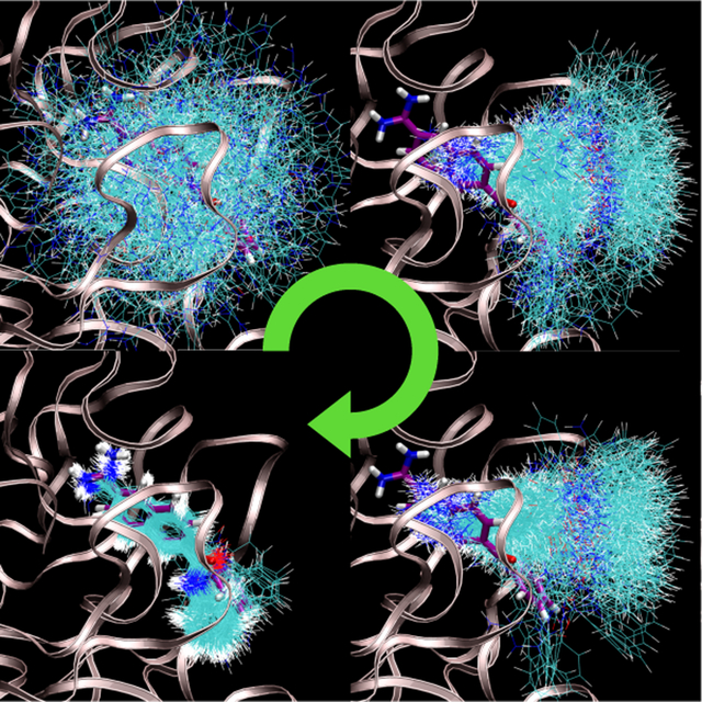
Configurations sampled from representative thermodynamic states as the temperature is reduced and receptor-ligand interactions are scaled in. These samples are used to estimate binding free energies between exible small molecules and rigid receptors. These estimates can be used for estimating binding free energies between exible binding partners.

INTRODUCTION

Alchemical Grid Dock (AlGDock) is an open-source computer program designed to compute the binding potential of mean force (BPMF) - the binding free energy between a flexible ligand and a rigid receptor - between a small organic ligand and a biological macromolecule.

The BPMF is defined as a ratio of configurational integrals¹,

$$B\left(r_R\right)=-{\beta }^{-1}\text{\hspace{0.17em}ln\hspace{0.17em}}\left(\frac{\int I\left(\xi \right)J\left(\xi \right)e^{-\beta U\left(r_{RL}\right)}d{r}_{L}d\xi }{\int I\left(\xi \right)J\left(\xi \right)e^{-\beta \left[U\left(r_L\right)+U\left(r_R\right)\right]}d{r}_{L}d\xi }\right).$$ (1)

In this paper, the internal coordinates (excluding translation and rotation) of a receptor-ligand complex, r_RL, are partitioned into the receptor, r_R, the ligand, r_L, and the relative translation and rotation of the species, ξ. β = (k_BT)⁻¹ is the inverse of Boltzmann’s constant times the temperature. I(ξ) is an indicator function that specifies whether the receptor and ligand are bound (1) or not (0). J(ξ) is the Jacobian for transforming Cartesian coordinates into the coordinate system used for r_L and ξ. U(·) is the potential energy of a species in solvent.

BPMFs are useful for characterizing noncovalent association processes. According to implicit ligand theory (ILT)^1,2, the standard binding free energy can be computed from BPMFs between a ligand and multiple receptor conformations. Moreover, ILT explains that BPMFs can reweight receptor conformations from the apo (ligand-free) to the holo (ligand-bound) ensemble for the ligand of interest. This approach has the greatest potential benefit when computing binding free energies or averages over respective holo ensembles for many ligands to a single receptor; after performing receptor sampling once, the same snapshots may be used for many ligands. Another potential use for BPMFs is as a secondary scoring function for molecular docking.

A number of BPMF calculations have been published in the scientific literature. In the first paper on ILT, BPMFs were estimated for simple host-guest systems¹. Unlike the calculations herein, the calculations in this first paper did not employ computational shortcuts that exploit the rigidity of the receptor. Without necessarily referring to their calculations as BPMFs, several groups have computed binding free energies between simple ligands and rigid conformations of the protein T4 lysozyme: Mobley et al.³ deployed rigorous alchemical binding free energy calculations; Ucisik et al.⁴ developed a fast and approximate method; and my research group published a study where BPMFs were computed using AlGDock⁵ and another where they were computed based on a fast Fourier Transform⁶. In my group’s former publications involving AlGDock, we cited an unpublished earlier version of this article⁷. In Xie et al.⁵, we computed standard binding free energies for 141 ligands using multiple BPMFs and showed that our results accurately reproduce values from flexible-receptor simulations for 25 ligands. The same BPMFs were used to demonstrate our new formalism for estimating relative, opposed to absolute, binding free energies². In the Drug Design Data Resource Grand Challenge 3, a blinded challenge for binding affinity and pose prediction, my research group submitted entries based on BPMFs⁸. For one system, vascular endothelial growth factor receptor 2, our submissions were among the most highly correlated with experiment. Results from our purely physics-based approach were competitive with methods using knowledge-based potentials, which were the best performers in the challenge. As discussed in Xie and Minh⁸, several issues led to weaker performance in other subchallenges, including the neglect of DMSO and SO₄ in the binding site of Cathepsin S and poor selection of receptor snapshots for free energy calculations with Janus Kinase 2 and Mitogen-activated protein kinase 14. Based on its uneven performance in the challenge, it appears that BPMF calculations show potential but further development is necessary before broader use. In this paper, I describe BPMF calculations for a variety of protein receptors: the Astex diverse set⁹, a curated database of 85 high-quality crystallographic structures of protein-ligand complexes with pharmaceutical or agrochemical interest.

AlGDock uses methods that are similar to those used in recent alchemical binding free energy calculations with a flexible receptor^10–12 and also implements algorithms that make BPMF calculations faster and more robust. As in other work, AlGDock performs Boltzmann sampling for a series of thermodynamic states with different degrees of coupling between the receptor and ligand and periodically attempts Monte Carlo moves to exchange configurations between the different replicas. The main methodological distinctions are (1) the use of precomputed nonbonded interaction grids for receptor-ligand interactions^13–15 and (2) the adaptive initialization and on-the-fly adjustment of thermodynamic states. The former accelerates BPMFs compared to flexible-receptor binding free energy calculations because evaluating nonbonded terms no longer scales as O(N²) (neglecting cutoffs) with the number of receptor atoms N. Rather, once the grid is computed, calculation time does not depend on N. The latter improves the precision of free energy estimates by ensuring sufficient configuration space overlap between adjacent thermodynamic states along the alchemical protocol.

AlGDock is a python module based on the Molecular Modeling Toolkit (MMTK) 2.7.8¹⁶. It is available under the open-source MIT license at https://github.com/ccbatiit/algdock/.

METHODOLOGY

This section details the algorithms in AlGDock and describes demonstrative BPMF calculations for the Astex diverse set⁹. Parameter values specified below, e.g. the binding site radius, were used in the demonstrative calculations, but most are adjustable arguments to the program.

Thermodynamic Cycle

In AlGDock, BPMFs are calculated based on the thermodynamic cycle shown in Figure 1. Figure 1 shows milestone thermodynamic states, which are referred to with the letters A to E. The states between and including milestones X and Y will be referred to as states XY.

Figure 1: Thermodynamic cycle for BPMFs.

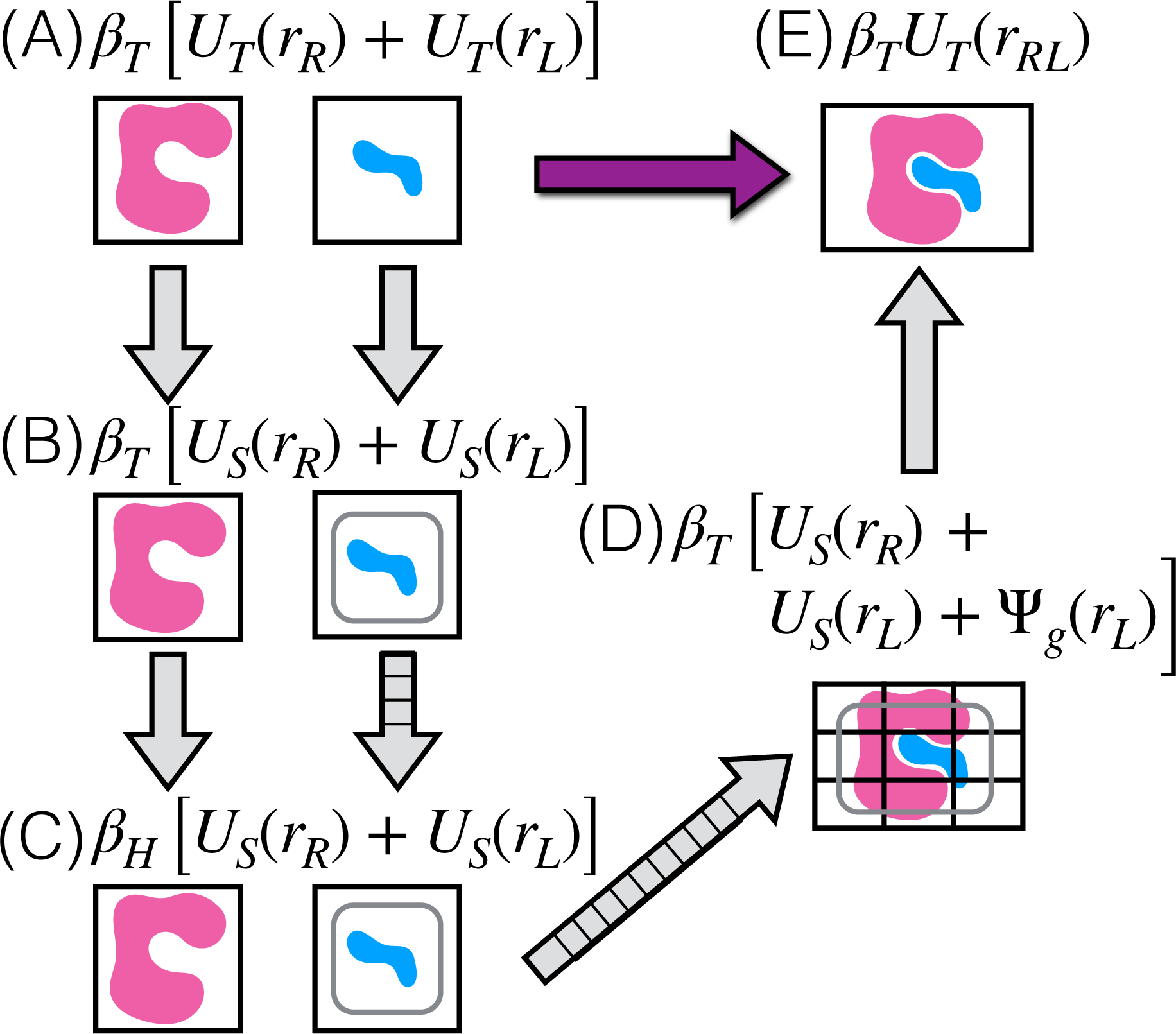
Milestone thermodynamic states are labeled with letters in parentheses and expressions for the reduced potential energy. ${\beta }_T^{-1}=k_B\left(300\text{\hspace{0.17em}K}\right)$ and ${\beta }_H^{-1}=k_B\left(600\text{\hspace{0.17em}K}\right)$ are inverse temperature factors for the target and high temperatures, respectively. U_T (·) and U_S(·) denote potential energies for the target and sampling force fields, respectively. These potential energies include molecular mechanics terms and the implicit solvent model. Ψ_g(·) is the potential energy due to receptor-ligand interaction grids. Arrows with orthogonal lines indicate multiple intermediate thermodynamic states. For BPMF calculations, configurations are sampled from thermodynamic states with the rounded boxes and from their intermediates.

Over the course of this cycle, the receptor-ligand interaction strength is scaled and the temperature is varied. The temperature is varied because high-temperature states enhance transitions between local energetic minima. As this paper will deal with thermodynamic states at different temperatures, I will frequently refer to the reduced potential energy¹⁷, a log probability density that incorporates the inverse temperature factor β = (k_BT)⁻¹. Reduced potential energies for key milestones in the thermodynamic cycle are shown in Figure 1. Subsequently, the reduced potential energy will be denoted with a lowercase u. Furthermore, the reduced free energy difference between two milestones X and Y will be denoted as f_XY. Because converting from reduced to standard potential energies and free energies involves dividing by β, the units of these reduced quantities are k_BT.

In all of the simulated thermodynamic states, the ligand is confined to the binding site using a flat-bottom harmonic potential^1,10,11,

$$u_I\left(d\right)=\{\begin{array}{ll}0\hfill & \text{\hspace{0.17em}if\hspace{0.17em}}d\le d_0\hfill \\ \frac{1}{2}\beta k{\left(d-d_o\right)}^2\hfill & \text{\hspace{0.17em}if\hspace{0.17em}}d>d_0\hfill \end{array},$$ (2)

where k = 10000 kJ/(mol nm²) is the spring constant, d is the distance between the ligand center of mass and the center of the binding site, and d₀ = 6.0 Å is the radius of the binding site. There is no restriction on ligand rotation.

The thermodynamic cycle involves sampling and target force fields, which may be distinct from each other. In the demonstrative calculations, the sampling and target force fields had much in common, but some important distinctions. They both used the AMBER ff14SB force field for proteins and ions and Generalized Amber Force Field 2¹⁸ with AM1BCC charges^19,20 for other molecules. The key differences between the target and sampling force fields were the solvation model and whether receptor-ligand interactions were evaluated directly or by grid interpolation. They were also implemented via different python modules. In the sampling force field, AlGDock uses MMTK (which was extended to include implicit solvent and grid interpolation terms) to calculate energies and forces. In contrast, the target force field was evaluated with OpenMM²¹. The sampling force field uses the generalized Born/surface area model II from Onufriev et al.²² (OBC), adapted from OpenMM²¹, as an implicit solvent model. It differs from the target force field because only the ligand, opposed to the entire complex, is assumed to be solvated, and because it is sometimes scaled down, as described in the next paragraph. Finally, the sampling force field models receptor-ligand interactions with grid interpolation, as described further below. In the target force field, these interaction energies are directly computed.

To elaborate on the implicit solvent model, the sampling force field in AlGDock can employ two solvation pathways: Desolvated and Full. In the Desolvated pathway, an implicit solvent model for the ligand is present in milestone B but its strength is linearly scaled down and is zero at milestone C. Implicit solvent is not used for states CD, saving computer time. This pathway makes the most sense if the bound ligand is nearly completely desolvated. In the Full solvation pathway, the implicit solvent is at full strength for states BD. This pathway makes the most sense if the bound ligand is nearly fully solvated. In either case, an implicit solvent model for the complex (opposed to just the ligand) is used in milestones A and E. Therefore, the final results for either solvation pathway should be equivalent in the limit of asymptotic sampling, but may be distinct for incompletely converged calculations.

The grid interaction energy,

$${\Psi }_g\left(r_{RL}\right)={\Psi }_{\mathit{\text{PBSA}}}\left(r_{RL}\right)+{\Psi }_{\mathit{\text{vdW}}}\left(r_{RL}\right),$$ (3)

is based on one electrostatic and two van der Waals grids.

The electrostatic interaction energy Ψ_PBSA(r_RL) is evaluated by multiplying atomic partial charges with the electrostatic potential. The electrostatic potential for each ligand configuration is obtained by trilinear interpolation of a precomputed grid. The grid is produced by solving the linear Poisson-Boltzmann equation around the minimized receptor molecule using APBS 1.4²³ with sequential focusing. Coarse grids are at least 1.5 times larger than the range of the receptor molecule in each dimension. Fine grids have the same size as the van der Waals grids, and a spacing of 0.5 Å. Coarse grids use multiple Debye-Huckel boundary conditions, and fine grids use coarse-grid solutions as boundary conditions. Both grids are solved with the following options: a quintic B-spline charge discretization, spline window width of 0.3, protein dielectric of 2.0, solvent dielectric of 80.0, solvent density of 10.0, solvent radius of 1.4 Å, smoothed dielectric and ion-accessibility coefficients, and temperature of 300.0 K.

The van der Waals interaction energy Ψ_vdW (r_RL) is evaluated by an analogous grid-based procedure¹⁵. This procedure is built on the ideas of Pattabiraman et al.¹³ and Meng et al.¹⁴, who precomputed van der Waals energies at positions along a grid. To account for the highly nonlinear nature of van der Waals potentials²⁴, energies are calculated using a transformation, trilinear interpolation, and inverse transformation²⁵. Based on my previous recommendation¹⁵, an inverse transformation power of 4 is used for the repulsive potential and no transformation for the attractive potential. (A reasonable alternative approach could be the logarithmic interpolation proposed by Diller and Verlinde²⁶.)

Alchemical transformations that modulate the strength of interactions between atoms often face an “end-point catastrophe” in which free energy changes are numerically unstable²⁷. The end-point catastrophe occurs because steric overlaps that do not lead to high energies when molecules are decoupled can do so when coupling is added. To circumvent this issue, a set of soft Lennard-Jones repulsive and electrostatic grids is introduced between milestones C and D. In these soft grids, the original grid value, v_o, is replaced with v_max tanh(v_o/v_max). (Gallicchio and Levy¹⁰ also used a hyperbolic tangent energy cap.) For the soft Lennard-Jones repulsive grid, v_max = 10.0 kJ mol^−1/2. A potential issue with soft Lennard-Jones is that they can be overwhelmed by electrostatic contributions. To circumvent this issue of electrostatic pinning, the soft electrostatic grid uses as maximum value such that the electrostatic energy is less than or equal to the soft Lennard-Jones repulsive energy for every heavy atom at every grid point. This is established by setting v_max for the electrostatic grid to 10 times the minimum ratio of Lennard-Jones and electrostatic scaling factors. The reduced potential energy is switched according to the protocol,

$$u_{\alpha }\left(r_{RL}\right)=\frac{1}{k_{B}T\left(\alpha \right)}\left[U_s\left(r_L\right)+U_s\left(r_R\right)+{\alpha }_{sg}\left(\alpha \right){\Psi }_{sg}\left(r_{RL}\right)+{\alpha }_g\left(\alpha \right){\Psi }_g\left(r_{RL}\right)\right]$$ (4)

$${\alpha }_{sg}\left(\alpha \right)=-{\left(2\alpha -1\right)}^2+1$$

$${\alpha }_g\left(\alpha \right)=\frac{{\left(2\alpha -1\right)}^2}{1+\text{exp\hspace{0.17em}}\left[-1000\left(\alpha -\frac{1}{2}\right)\right]}$$

$$T\left(\alpha \right)=\left(T_T-T_H\right)\alpha +T_H$$

This protocol turns on the soft grids first, and then the unperturbed grids (Figure 2). The potential is consistent with milestone C at α = 0 and milestone D at α = 1.

Figure 2: Grid scaling for states CD.

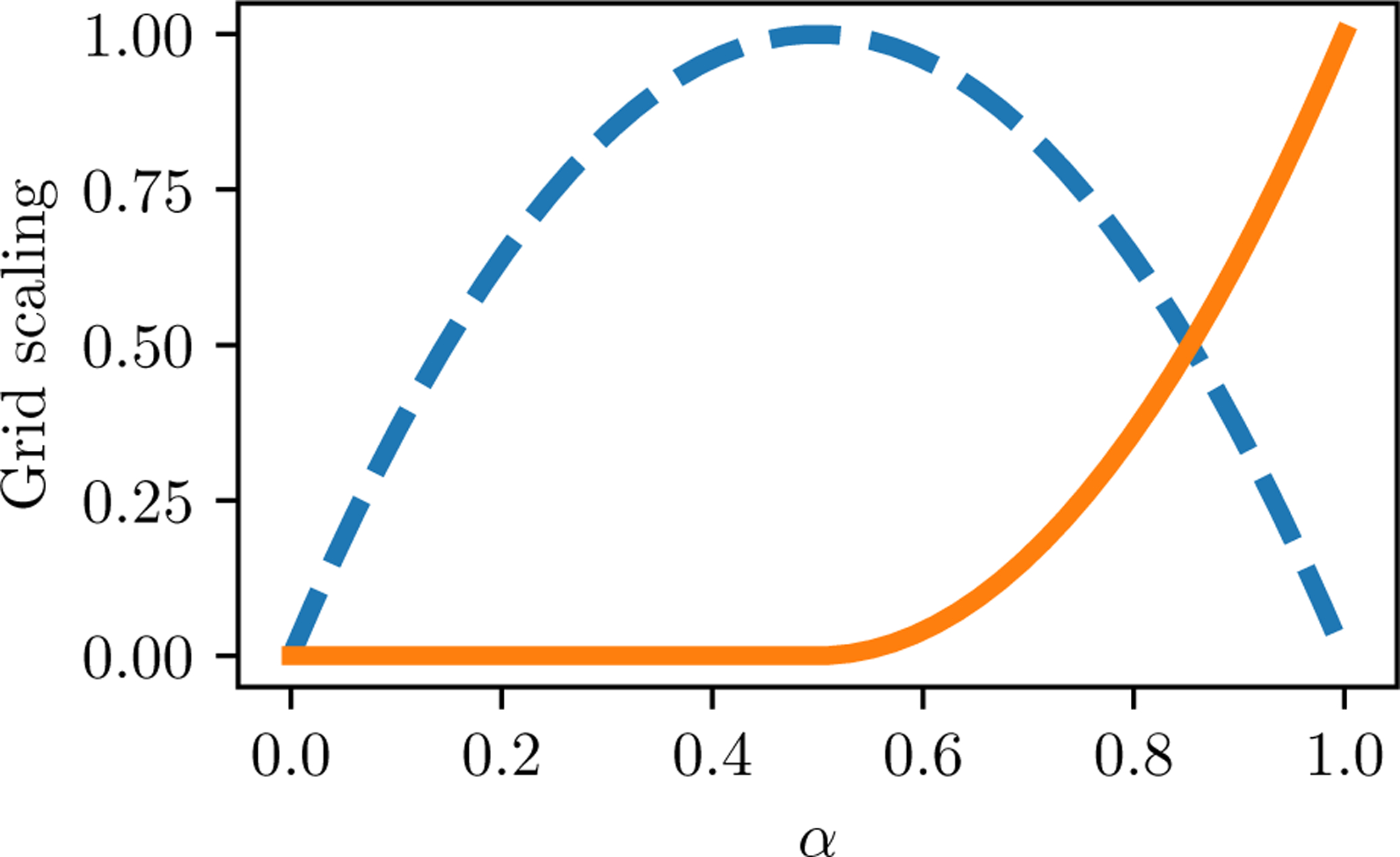
α_sg (dashed line) and α_g (solid line) as a function of the progress variable α.

Sampling

For states BD, ligand conformational sampling is performed with a combination of Hamiltonian Monte Carlo (HMC)²⁸, external coordinate Markov chain Monte Carlo moves, and Hamiltonian replica exchange.

HMC trial moves are based on 50 steps of velocity Verlet molecular dynamics with an adaptive time step that ranges between 0.1 and 5.0 fs. Time step adaptation occurs during the initialization of thermodynamic states, as described in the next section.

To accelerate transitions between binding poses, external coordinate Markov chain Monte Carlo moves are attempted for states CD when α < 0.01. The external coordinate move consists of:

1. Random rotation. A random quaternion is converted into a matrix that is used to rotate the molecule about its center of mass.

2. Random translation. The magnitude of translation in each dimension is drawn from a Gaussian distribution with a standard deviation of 0.6 Å.

The move is accepted or rejected according to the Metropolis criterion. Moves are not attempted for α > 0.01 due to low acceptance probability.

During production, Hamiltonian replica exchange^1,10,11,29 is attempted for states BC and states CD. Replica exchange is a Markov chain Monte Carlo move that swaps the configurations of a pair of simulations at different thermodynamic states. (Equivalently, it may be regarded as swapping the states.) Consider the thermodynamic states a and b with reduced energies u_a and u_b, respectively. If x is the original configuration in state a and y the original configuration in state b, then the acceptance probability,

$$p_{\mathit{\text{acc}}}=\text{min\hspace{0.17em}}\left[1,e^{-u_a\left(y\right)-u_b\left(x\right)+u_a\left(x\right)+u_b\left(y\right)}\right],$$ (5)

preserves the Boltzmann distribution in both states.

Typical replica exchange protocols attempt exchanges between pairs of neighboring thermodynamic states, but this restriction is unnecessary. As replica exchange is a type of Gibbs sampling³⁰, an arbitrary number of attempts can be made between arbitrary pairs of states. In AlGDock, each sweep of replica exchange includes attempts to swap configurations between pairs of states that are 1, 2, …, min(5, K) states apart, where K is the total number of thermodynamic states in the direction.

Stages

BPMF calculations with AlGDock are broken down into the following stages:

1. Ligand preparation: the ligand is minimized with 5000 steepest descent steps. The temperature is ramped from 20 K to 300 K over 30 geometrically spaced simulations of 2500 steps each.

2. Initialization: starting from 50 seed configurations, simulations of 2000 steps are used to initialize each thermodynamic state for states BD.

3. Equilibration and production: simulations are conducted for states BC and subsequently for states CD.

4. Postprocessing: samples from milestones B and D are postprocessed using the target force field.

5. Estimation: Free energy differences that sum up to the BPMF are estimated.

Initialization

The purpose of initialization is to establish a protocol with reasonable time steps and mean replica exchange rate 〈p_acc〉 between all neighboring states. The key benefit of replica exchange is to spread sampled configurations across a range of different thermodynamic states. A bottleneck in the exchange of configurations across the pair of states can eliminate this benefit of replica exchange; groups of thermodynamic states separated by the bottleneck effectively become independent. Low exchange probabilities are also indicative of poor configuration space overlap, which can limit the convergence of free energy estimates³¹.

For states BC, the first thermodynamic state (k = 0) is at 300 K and the ligand is steadily warmed to 600 K. The first thermodynamic state initialized for states CD depends on whether there is a fully-bound pose available in the binding site. If a pose is available, then the first state is fully bound at 300 K. Otherwise, the first state is fully unbound at 600 K. In the latter situation, 50 randomly selected configurations from milestone C are placed in the binding site at 453 random center-of-mass positions (0.5 positions per ų) and rotated with 100 different random orientations.

After state k is initialized, state k + 1 is initialized as follows:

1. Parameter selection: Parameters for state k + 1 are selected using a new algorithm designed to separate states at approximately even intervals in thermodynamic length.

   Thermodynamic length is a metric of the distance on the manifold of thermodynamic states³². For a sequence of states, the statistical error in free energy calculations is minimized and the replica exchange frequency is nearly maximized when intermediate states are equidistant in thermodynamic length³³. Suppose that thermodynamic parameters (e.g. temperature, pressure, grid scaling strengths) are specified by a vector λ with components λⁱ. Let γ ≡ γ(α) describe the dependence of λ on the variable α, such that γ(0) is the initial and γ(1) is the final thermodynamic state. For microscopic systems, the thermodynamic length is defined by the path integral^33,34,

   $$\mathcal{L}\equiv {\int }_0^1\sqrt{\sum _{i,j}\frac{\partial {\gamma }^i}{\partial \alpha }g{\left(\gamma \right)}_{ij}\frac{\partial {\gamma }^j}{\partial \alpha }}d\alpha .$$ (6)

   Given a parameter vector λ, the reduced potential energy is u_λ(x) = U_λ(x)/(k_BT_λ), where U_λ(x) is the effective potential energy and T_λ is the temperature. The normalized log probability of observing a configuration x is l_λ(x) = −u_λ(x) − lnZ_λ, where $Z_{\lambda }=\int e^{-u_{\lambda }\left(x\right)}dx$ is the partition function. These quantities are used to define elements of the Fisher information matrix,

   $$g{\left(\gamma \right)}_{ij}\equiv {\sigma }_{\lambda }^2\left[{\partial }^i{l}_{\lambda },{\partial }^j{l}_{\lambda }\right],$$ (7)

   where ${\sigma }_{\lambda }^2$ is the covariance in state λ and ∂ⁱ denotes a partial derivative with respect to λⁱ. For a protocol in which only one parameter λⁱ varies with α, the length is, $\mathcal{L}={\int }_0^1\frac{\partial {\gamma }^i}{\partial \alpha }{\sigma }_{\lambda }\left[{\partial }^i{l}_{\lambda }\right]dt$.
   Numerical estimates of $\mathcal{L}$ are most accurate when samples are drawn from many states between 0 < α < 1³⁴. Such exhaustive sampling, however, is unavailable during initialization. A simple approximation for the thermodynamic length when one parameter changes is, $\mathcal{L}=\Delta {\lambda }^i{\sigma }_0\left[{\partial }^i{l}_{\lambda }\right]$, where Δλⁱ is the total change in the value of the parameter λⁱ and σ₀ [∂ⁱl_λ] is a standard deviation in the initial state. Thus, if one desires $\mathcal{L}$ to be approximately constant between different intermediate stages in a protocol, then the change in parameter should be inversely proportional to σ₀ [∂ⁱl_λ],

   $$\Delta {\lambda }^i=\frac{s}{{\sigma }_0\left[{\partial }^i{l}_{\lambda }\right]},$$ (8)

   where s is an adjustable parameter, the thermodynamic speed.
   For example, with the Full solvation pathway, the parameter that varies between milestones B and C is the temperature, T. As the log probability of a ligand configuration is $l_{\lambda }=-\frac{U_S\left(r_L\right)}{k_{B}T}-\text{ln\hspace{0.17em}}{Z}_{\lambda }$, T is incremented by,

   $$\Delta {\lambda }^i=-\frac{s_{bc}k{T}^2}{{\sigma }_{\lambda }\left[U_S\right]},$$ (9)

   where s_bc = 20.0. For states CD, the log probability of r_RL is l_λ = −u_α(r_RL) − ln Z_λ. α is incremented by,

   $$\Delta {\lambda }^i=s_{cd}{\left[\left|\frac{d{\alpha }_{sg}}{d\alpha }\right|\frac{{\sigma }_{\lambda }\left[{\Psi }_{sg}\right]}{k_{B}T\left(\alpha \right)}+\left|\frac{d{\alpha }_g}{d\alpha }\right|\frac{{\sigma }_{\lambda }\left[{\Psi }_g\right]}{k_{B}T\left(\alpha \right)}+\left|T_T-T_H\right|\frac{{\sigma }_{\lambda }\left[u_{\alpha }\left(r_{RL}\right)\right]}{T\left(\alpha \right)}\right]}^{-1},$$ (10)

   with s_cd = 0.2. If the targeted value of the parameter is exceeded (e.g. temperature increased above 600 K), then the targeted value is used.

2. Seed selection: 50 configurations from state k are resampled as starting seeds for simulations in state k + 1.

   Configurations are drawn from state k with weights proportional to exp[u_k(x_i) − u_k+1(x_i)], where u_k(x) = U_k(x)/(k_BT_k) is the reduced potential energy in state k. In the limit of infinite sampling of state k, resampled configurations would be Boltzmann-distributed in state k + 1. With imperfect sampling of state k, resampled configurations approximate the Boltzmann distribution in state k + 1. The seed selection process is an example of what is known in the statistics literature as sampling importance resampling.

3. Sampling and adaptation: Simulations of 2000 steps are run from each seed and the sampling protocol is adapted to obtain a reasonable acceptance rate.

   If the Monte Carlo acceptance rate is greater than 0.8, the time step is increased by 0.125 fs. If it is less than 0.4, then the time step is reduced by 0.25 fs. If it is less than 0.1, then the time step is reduced by 0.5 fs. Initialization is repeated at the new time step until the acceptance rate is between 0.4 and 0.8.

4. Verification: The mean replica exchange probability, 〈p_acc〉, is used to verify that thermodynamic states are not too distinct nor similar.

   It is estimated by taking the sample mean of p_acc (Eq. 5) for every pair of initial samples (at the same time index) from states k and k + 1. If 〈p_acc〉 is estimated to be too low³⁵ (below 0.4), then parameters for state k + 1 are reselected with a smaller increment (thermodynamic speed is adjusted by a factor of 4/5) and simulations are repeated. If it is too high (above 0.99), then state k is removed.

Equilibration and production

Equilibration and production calculations are broken down into cycles. Each cycle consists of 1000 iterations of the following: an HMC move and 20 external coordinate MCMC moves (if α < 0.01) for each thermodynamic state and then 25 sweeps of replica exchange. 50 snapshots are saved per replica exchange cycle. The demonstrative calculations are based on 8 cycles between for states BC and 15 cycles for states CD.

Between each cycle, simulation data are saved and thermodynamic states are inserted as necessary. The purpose of inserting thermodynamic states is to ensure adequate replica exchange acceptance rates. As discussed above, AlGDock includes an estimate of 〈p_acc〉 to verify new thermodynamic states during initialization. However, the configuration space explored during replica exchange can be distinct from that explored during initialization, leading to a substantial change in the observed p_acc. Thus, if at the end of a cycle the average replica exchange acceptance rate between any pair of neighboring thermodynamic states falls to less than 0.4³⁵, then another thermodynamic state is inserted between the pair. Sampling importance resampling is used to populate configurations in this new state. That is, samples for the new state are drawn from samples for other states with probability proportional to the density in the new state.

Separation of equilibration and production is based on a method inspired by Chodera³⁶. The integrated autocorrelation time and statistical inefficiency is estimated based on the mean potential energy of configurations from the last c ∈ {1, 2, …, C} cycles of equilibration and production, where C is the total number of cycles. The number of statistically independent samples is determined by dividing the number of snapshots in c cycles by the estimated statistical inefficiency. The simulation is considered equilibrated based on the value of c that provides the largest number of statistically independent samples.

Estimation

BPMFs were estimated according to ${\beta }_{T}B\left(r_R\right)=f_{AB}+f_{BC,L}+f_{CD}^{\prime }+f_{DE}.f_{BC,L}$ is the free energy of warming the ligand from T_T = 300 K to T_H = 600 K, and,

$$f_{CD}^{\prime }=-\text{ln}\frac{\int I\left(\xi \right)J\left(\xi \right)e^{-{\beta }_T\left[U\left(r_L\right)+{\Psi }_g\left(r_{RL}\right)\right]}d{r}_{L}d\xi }{\int I\left(\xi \right)J\left(\xi \right)e^{-{\beta }_{H}U\left(r_L\right)}d{r}_{L}d\xi }.$$ (11)

$f_{BC,L}+f_{CD}^{\prime }$ is used instead of f_BC + f_CD because the former calculation can be performed without determining the receptor internal energy U(r_R). The receptor desolvation free energy is estimated by the difference, f_AB,R = β_T (U(r_R) − U(r_R)). Other free energy differences are estimated based on equilibrated samples from replica exchange for states BC or states CD. f_AB,R and f_DE are estimated by free energy perturbation³⁷ using configurations drawn from milestones A and E, respectively. f_BC,L and $f_{CD}^{\prime }$ are estimated by the multistate Bennett acceptance ratio¹⁷, which uses potential energies from every replica.

Pose prediction

Binding poses were predicted based on ligand conformations sampled after equilibration. Configurations sampled from milestone D were clustered using hierarchical clustering with complete linkage, performed using scipy.cluster.hierarchy.linkage in scipy v0.14.0³⁸. Distances between snapshots were based on the Hungarian symmetry-corrected heavy-atom root mean square deviation (RMSD), which is also implemented in UCSF DOCK 6³⁹. Clusters were separated based on a threshold of 1.0 Å. The probability of each cluster was obtained by reweighing configurations via the factor,

$$w_c=\text{exp\hspace{0.17em}}\left[-{\beta }_T\left(U_T\left(r_{RL}\right)-U_S\left(r_L\right)-{\Psi }_g\left(r_L\right)\right)\right].$$ (12)

or by assuming that interaction energies are the only terms that change between milestones D and E,

$$w_c=\text{exp\hspace{0.17em}}\left[-{\beta }_T\left(U_T\left(r_{RL}\right)-U_T\left(r_L\right)-{\Psi }_g\left(r_L\right)\right)\right].$$ (13)

Pose predictions were based on the lowest-energy configuration, according to the force field in milestone E, from each cluster. Reduced free energies of each pose p were based on the cumulative weight of configurations in the cluster,

$$f_{E{E}_p}=-\text{ln}\frac{{\sum }_c{w}_c}{{\sum }_p{\sum }_c{w}_c},$$ (14)

where w_c is the weight of the configuration, ${\sum }_c$ is over configurations in the cluster, and ${\sum }_p$ is a sum over poses. If multiple independent simulations were run, the pose was predicted based on the pose with the lowest interaction energy, lowest total energy, or by the lowest pose-specific BPMF,

$$f_{AE,p}=f_{AE}+f_{E{E}_p}$$ (15)

Astex diverse set BPMF calculations

For each system in the Astex diverse set⁹, 11 independent simulations were performed using the Desolvated and Full solvation pathways. Input files in AMBER format (based on the ff14SB force field for proteins and ions and Generalized Amber Force Field 2¹⁸ with AM1BCC charges^19,20 for other molecules) were reused from a previous study¹⁵. Simulations were started from the crystallographic pose and poses obtained from molecular docking. Docking with UCSF DOCK 6³⁹ was repeated using a similar procedure as in the previous study¹⁵, but with a minimum anchor size of 5 instead of 40, which increases binding pose sampling.

After starting poses were minimized for 1000 conjugate gradient steps in the appropriate force field for milestone D, the lowest-energy pose was used to initialize simulations in the milestone. After the thermodynamic states were initialized, docked poses within the binding site were also used as starting points for each state in replica exchange. The lowest-energy pose was used for replica exchange with milestone D. Higher-energy poses were used in intermediate replicas to fill all available thermodynamic states. If there were more states than docked poses, the lowest-energy pose was duplicated.

Calculations were performed the Open Science Grid⁴⁰, supercomputing resources managed by the National Science Foundation eXtreme Science and Engineering Discovery Environment (XSEDE)⁴¹, and on the Minh group computing cluster at IIT. Benchmark calculations were run using single-core jobs with standard compute nodes on XSEDE Comet of the San Diego Supercomputer Center. These nodes have Intel Xeon E5–2680v3 processors, 128 GB DDR4 DRAM (64 GB per socket), and 320 GB of SSD local scratch memory.

RESULTS

Thermodynamic state initialization and adaptation is system-specific and robust

The described method for thermodynamic state initialization and adaptation yields protocols that are tailored for specific systems. The large range in the number of thermodynamic states, N_states, provides evidence that protocols are system-specific (Figure 3). For states BC, there is generally larger number of states with the Desolvated pathway (between 67 and 182) than for the Full pathway (between 51 and 111). The larger number of states is likely because of a more significant difference between the end states with the Desolvated pathway due to the removal of implicit solvent at milestone C. In contrast, the number of states for the Desolvated and Full pathways for states CD is comparable.

Figure 3: Number of thermodynamic states.

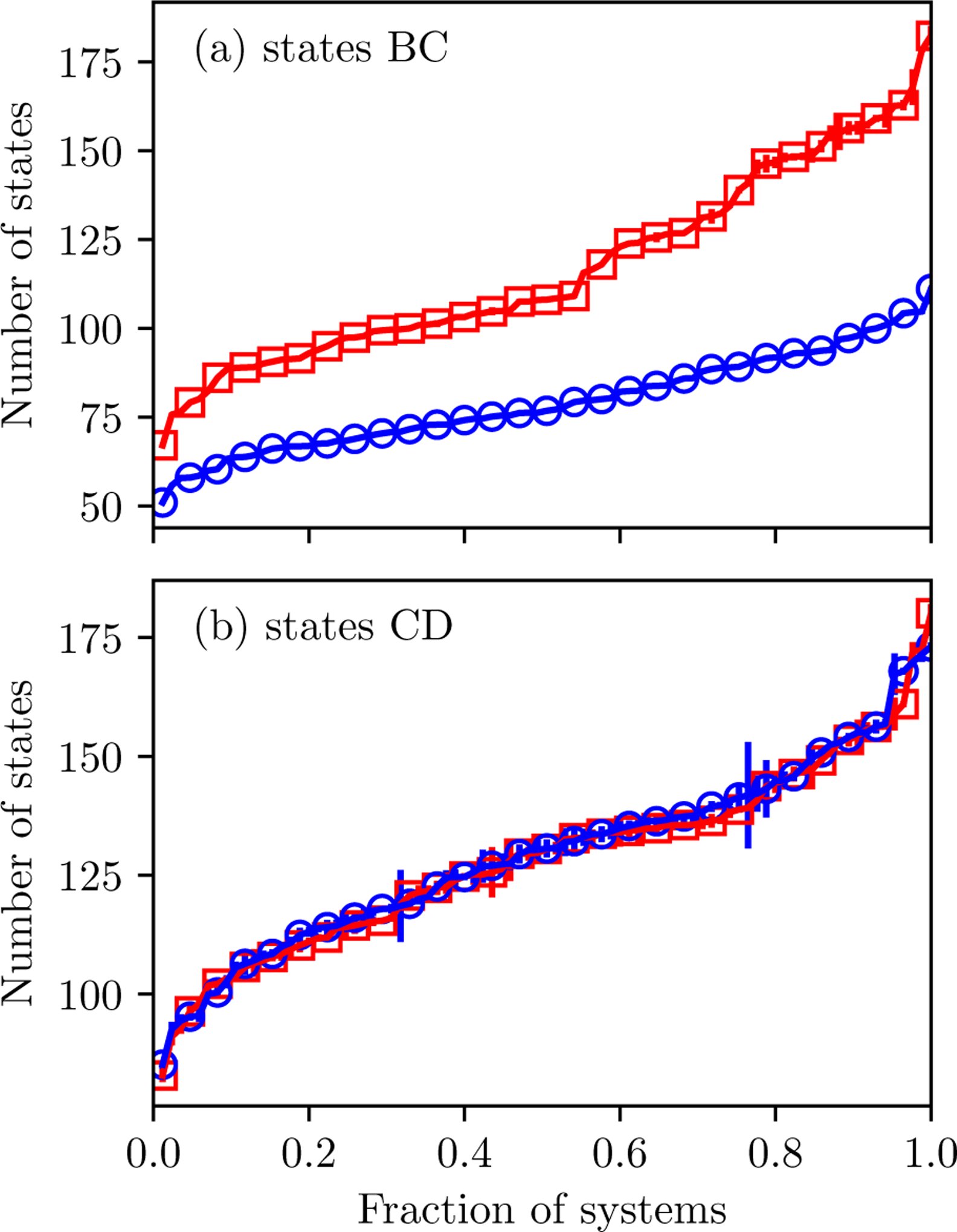
(a) for states BC, and (b) for states CD. The marker indicates the mean value and error bars the standard deviation of 11 independent simulations based on the Desolvated (red squares) and Full (blue circles) solvation options. They are ordered by the mean number of states.

In addition to being system-specific, the protocols appear to be robust. In all the systems, the standard deviation of the number of states, σ[N_states] is small relative to the average number of states, ${\overline{N}}_{\mathit{\text{states}}}$. For states BC, σ[N_states] is less than 2 for all systems. For states CD, the protocols are more variable. Variability may be larger because interaction grids introduce more possibilities for trapping in local minima during initialization. For 1l7f, the protocols for state CD appear to fall into two distinct classes (Figure S1 in the Supplementary Material). It is worth noting, however, that higher variation in protocols does not necessarily lead to inaccurate or imprecise results.

Similarly, the initialization of each state appears to be adaptive and robust. In the vast majority of initialization processes, the time step converged to between 2.75 and 3.75 fs (Figure S2 in the Supplementary Material). For states CD, some protocols have shorter time steps. The shortest time steps are from simulations with 1lrh. The relationship between the progress variable α and time step is fairly consistent across the independent protocols, demonstrating that the time step adaptation procedure is robust.

Replica exchange acceptance probabilities are reasonable

Estimates of 〈p_acc〉 indicate that protocols do not have any replica exchange bottlenecks (Figure 4). The notation ${\overline{p}}_{\mathit{\text{acc}}}$ refers to a statistical estimator for 〈p_acc〉. For states BC, ${\overline{p}}_{\mathit{\text{acc}}}$ estimated during replica exchange are high and have low variance. This outcome is consistent with achieving the goal of nearly equal thermodynamic length between adjacent thermodynamic states. It also implies that the configuration spaces explored during initialization and replica exchange are largely the same. For states CD, the replica exchange rates are also high but there is a larger variance. While most ${\overline{p}}_{\mathit{\text{acc}}}$ are between 0.7 and 1.0, there are a few simulations where ${\overline{p}}_{\mathit{\text{acc}}}$ is much lower. In these simulations, the acceptance probability dips around α = 0.2 or α = 0.8, but are high for most other values of α. These drops indicate that different conformations are explored in replica exchange compared to during thermodynamic state initialization. However, even these low ${\overline{p}}_{\mathit{\text{acc}}}$ are not low enough to be considered a bottleneck; they are expected to allow configurations to pass through the thermodynamic states several times per cycle.

Figure 4: Mean acceptance probability statistics.

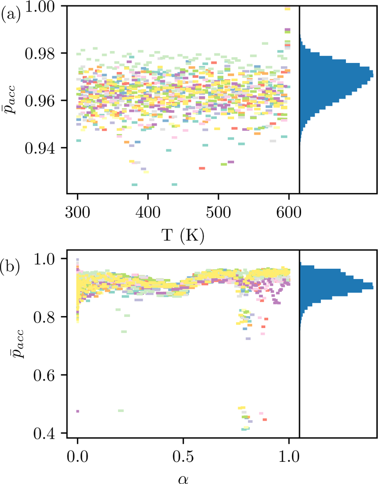
${\overline{p}}_{\mathit{\text{acc}}}$ for fifteen protocols with the lowest observed ${\overline{p}}_{\mathit{\text{acc}}}$ (a) for states BC and (b) and states CD are shown with the a line connecting neighboring states. Histograms of ${\overline{p}}_{\mathit{\text{acc}}}$ from all simulations are shown on the right panel. The largest bin count is 14492 for states BC and 31068 for states CD. For states CD, the simulations are from 1opk (4), 1r1h (4), 1t40 (3), 1v48 (2), 1oq5 (1), 1jje (1), where the number of simulations is in the parentheses.

The observed ${\overline{p}}_{\mathit{\text{acc}}}$ also underscore the point that large variation in protocols is not necessarily problematic. While some systems have a relatively large variation in N_states for states BC, all ${\overline{p}}_{\mathit{\text{acc}}}$ estimated from replica exchange are 0.92 or greater. Longer protocols simply have a higher ${\overline{p}}_{\mathit{\text{acc}}}$.

Simulation time is dependent on the solvation time and ligand size

The total CPU time of benchmark simulations spanned a large range (Figure 5). For simulations with the Desolvated option, they ranged from 4 to 44 hours. For simulations with the Full solvation option, they ranged from 6 to 117 hours.

Figure 5: Benchmark simulation times.

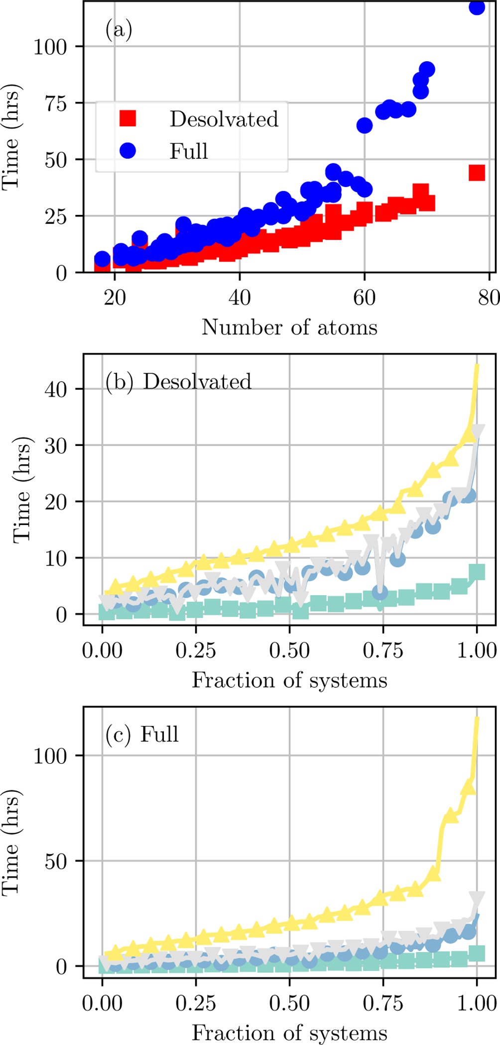
(a) Scatter plot of the total time for Desolvated (red squares) and Full (blue circles) solvation options as a function of the number of atoms in the system. Breakdown of times for (b) Desolvated and (c) Full solvation options. Benchmark simulations include initialization, equilibration and production, postprocessing, and free energy estimation. From bottom to top, lines depict the cumulative time through initialization (cyan squares) and estimation (violet circles) for states AC and then initialization (pink downward triangles) and estimation (yellow upward triangles) for states CE. Systems are ordered along the x axis by the total simulation time.

Benchmark simulation times are dependent on the solvation option and are roughly exponentially dependent on ligand size (Figure 5a). Simulations with the the Full solvation option are substantially slower than those with the Desolvated option, particularly for larger ligands. For both solvation options, the dependence appears roughly linear up to 40 atoms. Above this threshold, the difference in computation time between solvation options becomes more pronounced.

In all simulations, the majority of time was spent in equilibration and production (Figure 5b and 5c). The largest fraction of time was states CD, and the second largest fraction for states BC. Initialization and estimation for states CD consumes a small but noticeable fraction of simulation time, whereas the analogous steps for states BC consume a nearly negligible fraction of simulation time.

Simulations sample a variety of poses

At milestone C, sampled configurations are uniformly distributed in a sphere. As α increases from 0 to 1 for states CD, the configuration space of the ligand is gradually restricted. First, the soft grids prevent ligand atoms from overlapping with receptor atoms. At intermediate values of α, the ligand may assume several poses (e.g. Figure 6). Finally, at milestone D, the ligand usually but does not always sample from a single minimum.

Figure 6:

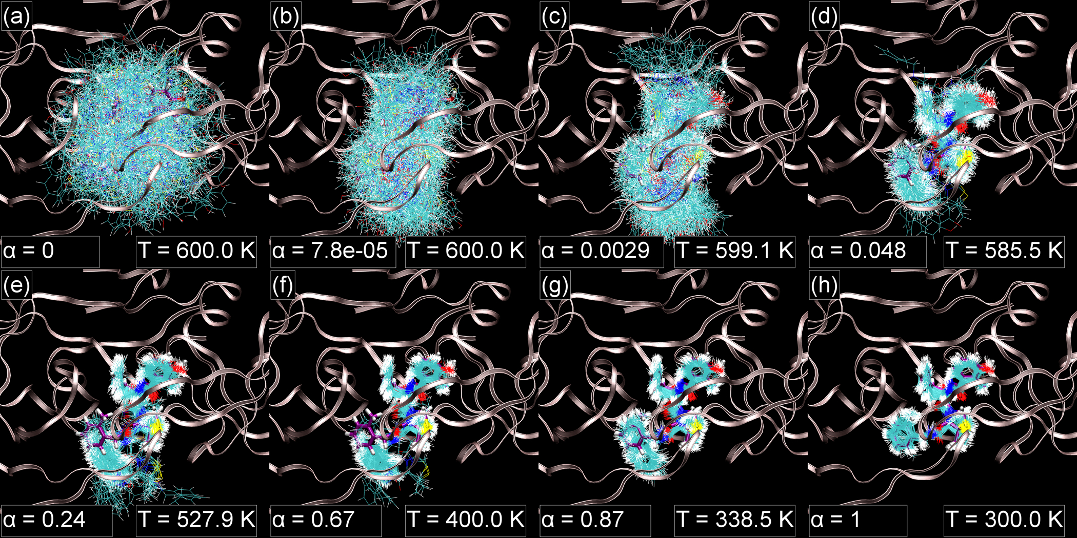
Samples from evenly spaced thermodynamic states for states CDx, taken from a representative simulation of 1kzk with the Desolvated solvation option. The protein structure structure is shown with ribbons and the crystallographic ligand pose is shown with a thick licorice representation and purple carbon atoms. The same illustration scheme is used in Figures 7 and 8. These figures were generated with VMD⁴⁹.

In many simulations, the configuration space sampled at higher α is a subset of that sampled at lower α (e.g. Figure 6). In others, however, the conformational minima for α ≈ 0.5, where the soft grids are at full strength, are entirely distinct from the minima for α ≈ 1 (e.g. Figure 7). When there are shifts in important configuration space, the thermodynamic states at α ≈ 0.5 are less beneficial to sampling from milestone D. Nonetheless, configuration space overlap between adjacent states is a sufficient condition for precise free energy estimates.

Figure 7:

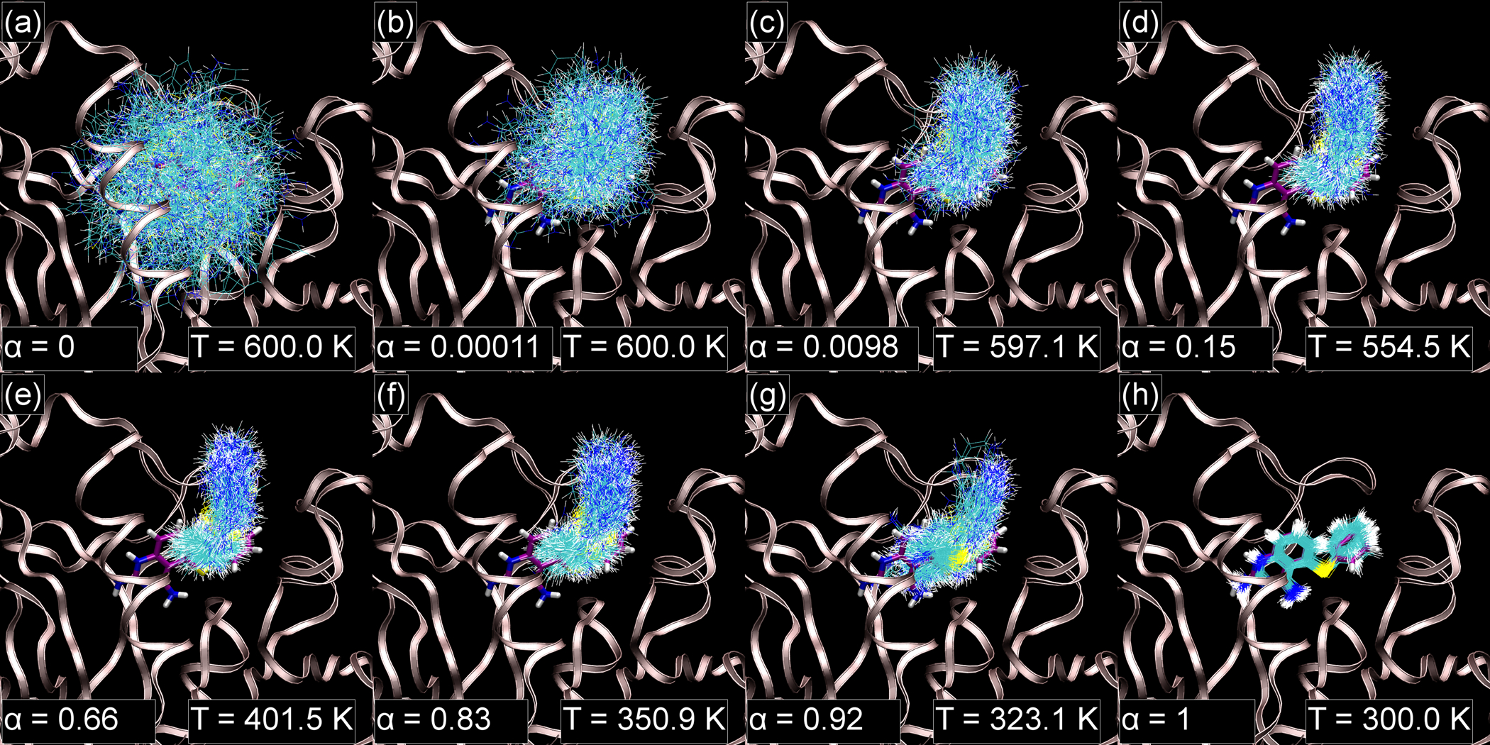
Samples from evenly spaced thermodynamic states for states CD, taken from a representative simulation of 1l7f with the Full solvation option.

At milestone D, most simulations sample from a single minimum (Figure 8ab), but there are several other situations. These include sampling alternate poses that share a common warhead position, but have a floppier tail (Figure 8cd), or that are clearly distinct (Figure 8efgh). When there are distinct poses, the native pose is often correctly identified as being most populated (Figure 8e), but sometimes other poses are calculated to have greater weight (Figure 8fgh). Indeed, the native pose may not even been among the predicted poses (Figure 8gh).

Figure 8:

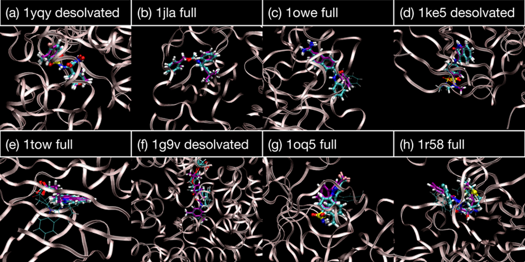
Predicted poses taken from representative simulations. A licorice representation is used for both the crystallographic pose (purple carbon atoms) and predicted poses (cyan). For the pose predictions, the thickness of the representation is proportional to its Boltzmann weight (using energies from the OBC model). Poses are shown for which weights are greater than 0.001.

Complex force field transfer limits BPMF precision

The mean and standard deviation of free energy differences between all adjacent pairs of milestones in the thermodynamic cycle (Figure 1) and for the total BPMF are reported in Table S1 of the supplementary material. While BPMFs are estimated within chemical precision of 1 kcal/mol = 1.68 RT for only 28.2% of systems, the majority of BPMFs are estimated within 4 k_BT (75.3% with Desolvated and 74.1% with Full options) and nearly all within 8 k_BT (87.1% with Desolvated and 94.1% with Full). The largest source of imprecision is estimation of f_DE, which is associated with transferring the complex between sampling and targeted force fields.

With the exception of f_DE, free energy differences between pairs of adjacent milestones in the thermodynamic cycle are feasible to calculate with AlGDock, converging quickly or at a steady rate. To evaluate the convergence of these estimates as a function of simulation time, the root mean square error (RMSE) between estimates for a particular cycle and estimates after the final cycle (for a particular solvation option) is considered. In the final cycle, the RMSE is simply the standard deviation. The fraction of systems with RMSE less than certain values is reported for different numbers of cycles in Figure 9.

Figure 9:

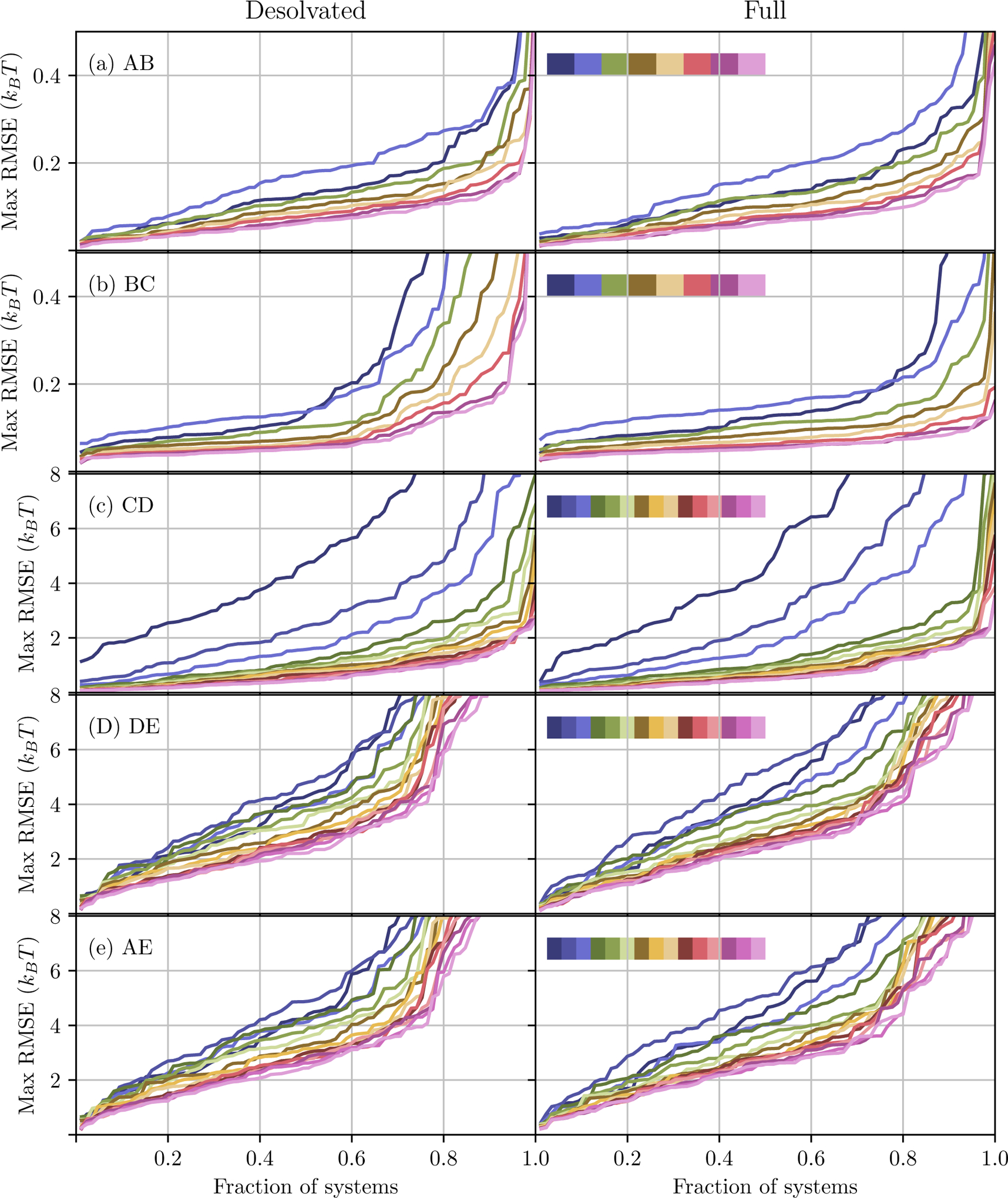
Fraction of systems with free energy differences calculated within a certain root mean square error of the final value. The rows are for free energy differences between different pairs of milestones. The columns are for the Desolvated (left) and Full (right) solvation options. Each line indicates a different number of cycles, with a total of 8 for the top two rows and 15 for the remainder. In the sequence of colors inset in the right column of each row, the color indicate an increasing number of cycles from left to right.

The free energy difference between milestones A and B, associated with transferring the ligand between the sampling and target force fields, converges quickly. After the first cycle, the RMSE of f_AB is less than 1 k_BT for all systems. After eight cycles, it is less than 0.5 k_BT for all but one set of calculations, 0.544 k_BT for 1p62 with the Desolvated option. The fast convergence of f_AB is expected because milestones A and B are meant to be the same force field, but simply evaluated using different software packages. Convergence is only dependent on adequate sampling of milestone B.

The free energy difference between milestones B and C, associated with changing the temperature of the ligand (and removing implicit solvent in the Desolvated option), also converges quickly. For the Desolvated option, the RMSE of f_BC is less than 2 k_BT for all but 1jje (3.2 k_BT) after the first cycle and less than 1 k_BT after eight cycles. The Full option converges more quickly, with a RMSE within 1 k_BT after one cycle and within 0.15 k_BT after eight. The faster convergence of the Full option is reasonable because milestones B and C are both in implicit solvent, implying that the protocol involves moving across a smaller region of configuration space.

The free energy difference between milestones C and D, associated with changing the temperature of the ligand and scaling the receptor-ligand interaction grid, converges more slowly than between milestones B and C. For the Desolvated option, the RMSE of f_CD is over 8 k_BT for 23 systems after one cycle. However, after 15 cycles, the RMSE is below 2.5 k_BT for all but one system, 2.65 k_BT for 1t40. For the Full option, the RMSE of f_CD is over 8 k_BT for 28 systems after one cycle. However, after 15 cycles, it is likewise below 2.5 k_BT for all but one system, 3.41 k_BT for 1l7f. For both solvation protocols, the RMSE of f_CD is below 2 k_BT for about 80% of systems after five cycles (Figure 9). It is reasonable that f_CD converges more slowly than f_BC because adding protein-ligand interactions leads to many local minima that simulations may become trapped in.

In contrast to the other pairs of milestones, the free energy difference between milestones D and E does not converge quickly nor at a steady rate for as many systems. For the Desolvated option, the RMSE is above 8 k_BT for 26 systems after one cycle. After 15 cycles, it is still above 8 k_BT for 9 systems. For the Full option, the RMSE is above 8 k_BT for 23 systems after one cycle and 5 systems after 15 cycles. With both protocols, the RMSE is below 2.5 k_BT for about 60% of systems and 4 k_BT for about 80% of systems. After about 5 cycles, the speed at which precision improves substantially slows. Given minimal changes in RMSE after about 12 cycles, it is unlikely that extending simulation beyond 15 cycles would lead to significant reduction in RMSE.

The convergence of f_DE appears to be the limiting factor in the convergence of the BPMF. If the convergence of the total BPMF were limited by different pairs of milestones depending on the system, then the RMSE curves in the final row of Figure 9 would differ from any other row. If one particular pair of milestones always limits the convergence of total BPMF, the curves on the bottom row would resemble curves for that pair of milestones. In the data, the RMSE curves in the penultimate and final row of Figure 9 are nearly identical.

Full solvation is less susceptible to false convergence

The prior discussion of standard deviations and RMSEs neglects the possibility of false convergence. False convergence occurs when thermodynamic expectations and free energy differences are apparently stable, even across multiple independent simulations, but simulations do not truly sample from the relevant configuration space. In general, false convergence is difficult to diagnose. However, in the context of AlGDock calculations, it is possible to compare results from the Desolvated and Full solvation options. For these options, although intermediate milestones differ, milestones A and E are equivalent and calculations should, in principle, lead to the same total BPMF.

Figure 10 shows free energies from a representative pair of simulations that take different pathways but yield nearly equivalent BPMFs. f_AB is the same pair of states for both pathways. The magnitude of f_BC is larger for the Desolvated pathway, consistent with the removal of implicit solvent in addition to the temperature change. f_CD has a similar overall shape. The BPMFs match because f_DE have opposite signs.

Figure 10:

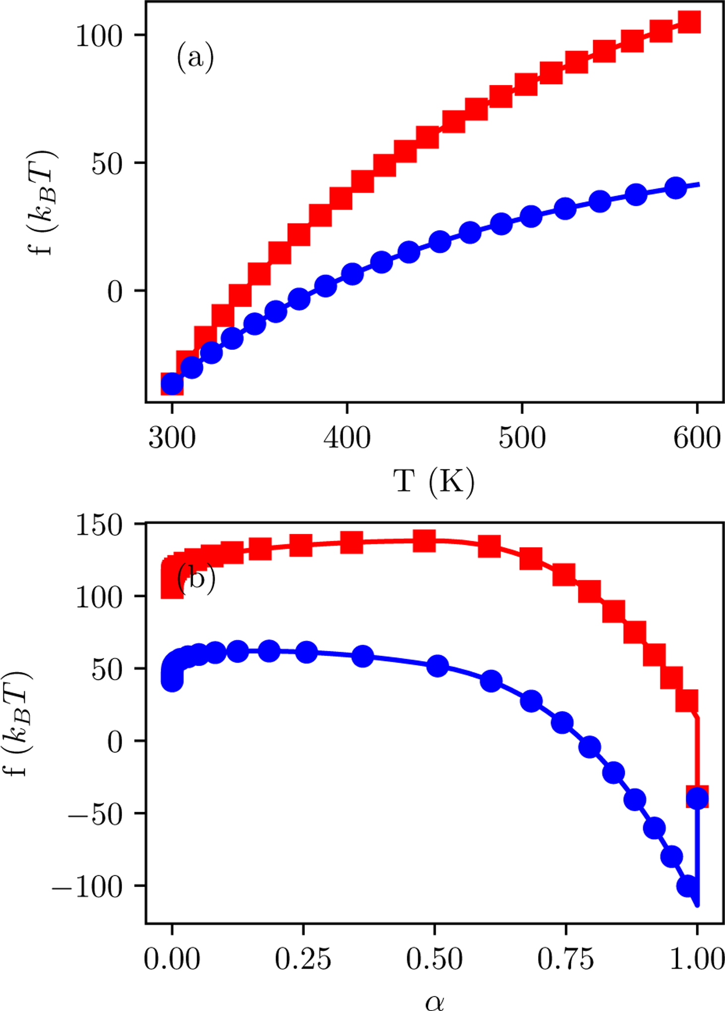
Representative cumulative free energies as a function of progress for states (a) AC and (b) DE for Desolvated (red squares) or Full (blue circles) options. Simulations are of PDB ID 1gpk. Panel (a) is based on the sum of f_AB and the free energy difference between T_T = 300 K and the temperature on the x axis. Panel (b) is based on the sum of f_AC and the free energy difference between α = 0 and the progress variable on the x axis. The final point on the plot shows f_AE for both pathways. For clarity, markers are shown only every four thermodynamic states.

In the majority of systems (63 systems or 74.1%), the mean BPMF from Desolvated and Full solvation options is within error (the sum of standard deviations for each of the estimates). In other cases, either the mean BPMF from Desolvated (5 systems) or Full (17 systems) solvation options is lower (Figure 11). Most of these differences are less than 10 k_BT, but several are very large, up to around 100 k_BT.

Figure 11: Differences between the mean BPMF of Desolvated and Full solvation options.

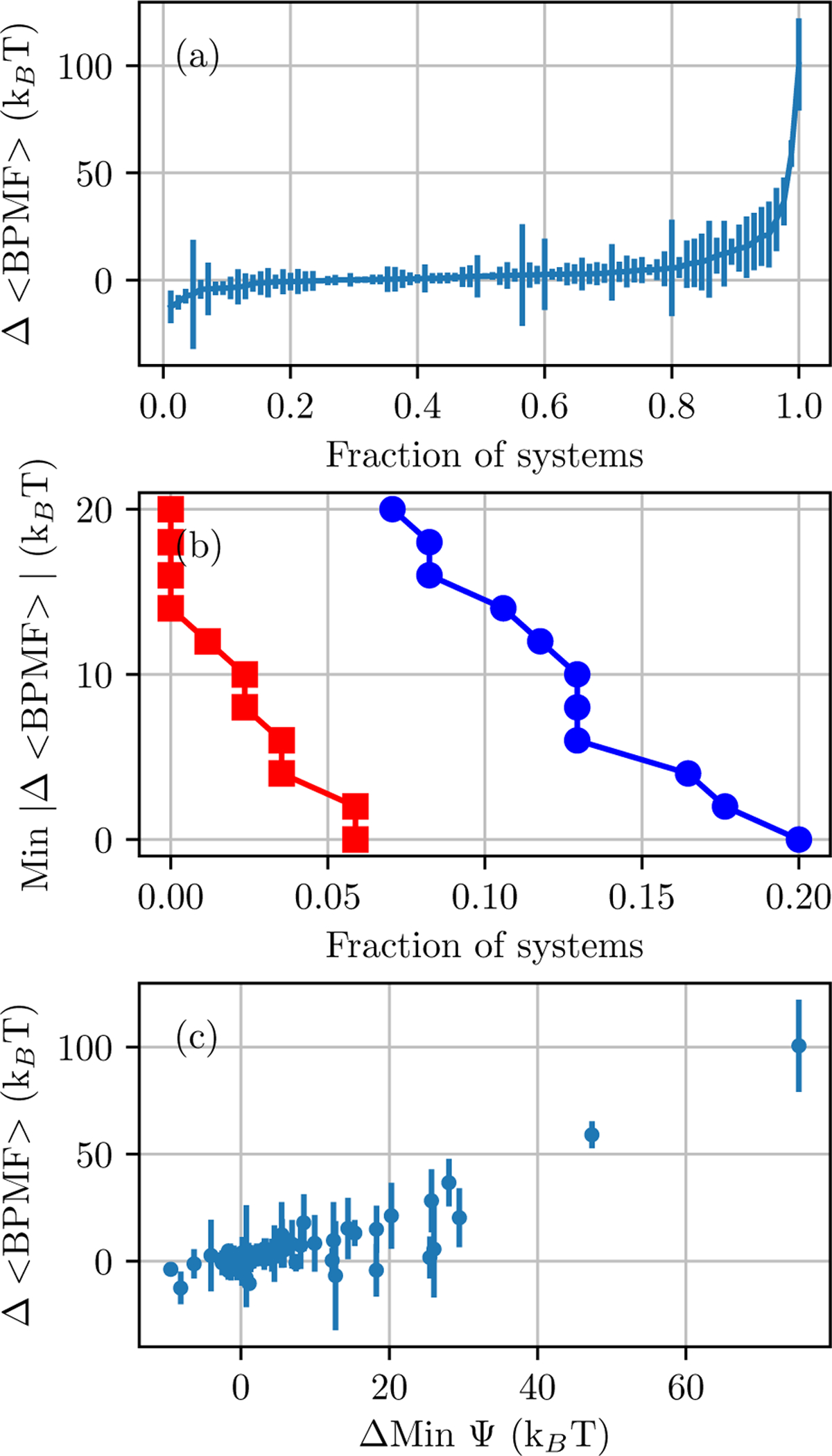
(a) Data points are ordered by the difference in mean BPMFs and the error bars are the sum of the standard deviations of the two estimates. (b) The fraction of systems in which the difference in mean BPMFs is larger than the sum of standard deviations of the two estimates. Either the Desolvated (red squares) or Full (blue circles) BPMF is lower by at least a certain value. (c) The difference in the minimum interaction energy, according to the force field in milestone E, versus the difference in mean BPMFs.

To facilitate analysis of false convergence, the consensus BPMF was defined as the lower of mean BPMFs for the two solvation options. The RMSE was computed relative to the consensus BPMF rather than the final BPMF observed for a specific solvation option. The fraction of systems with RMSE less than certain values is reported for different numbers of cycles in Figure S3 of the Supplementary Material. Reflecting its higher propensity for false convergence, the curves for the Desolvated option are noticeably shifted up and to the left compare to the RMSE versus the final value. After the last cycle, many systems still have high RMSEs relative to the consensus: 35.2% > 5 k_BT, 15.2% > 8 k_BT, 11.7% > 20 k_BT, and 9.4% > 30 k_BT. Curves for the Full option are shifted upwards more subtly. After the last cycle, fewer systems still have high RMSEs relative to the consensus: 35.2% > 4 k_BT, 24.7% > 5 k_BT, and 9.4% > 8 k_BT. The largest RMSE is 12.8 k_BT.

Convergence is limited by differences in sampled configuration space

The false convergence observed in some simulations is caused by differences in the important configuration space of milestones D and E. In general, the convergence of calculated free energy differences between a pair of thermodynamic states is facilitated by overlap of the configuration space important to the states⁴². The described f_DE calculations are based on samples from milestone D. If the configuration space important to milestones D and E differ, then sampling configurations important to milestone E using simulations of milestone D is a rare event.

Although it is difficult to determine whether the important configuration space of milestone E has been adequately sampled, it is feasible to compare the configuration space assessed with different solvation options. If they do access the same space, then it is reasonable to expect f_DE and BPMF estimates to be consistent. If they do not, then f_DE and thereby BPMFs are likely to be different. One way to quantify whether simulations access the configuration space important to milestone E is the minimum interaction energy, according to the force field used in milestone E. In a significant subset of systems, the minimum interaction energy observed in samples from milestone D with the two solvation options substantially differs (Figure 11c). Indeed, large differences the minimum interaction energy appear to be a necessary, but not sufficient, condition for large differences in BPMFs between the Desolvated and Full solvation options. That is, all cases with large differences in BPMFs also have large differences in the minimum interaction energy. However, there are a few cases in which large differences in the minimum interaction energy do not correspond to large differences in the mean BPMF.

While it may be intuitive to think that large differences in the mean interaction energy are due to large differences in binding poses, the data suggest that this is not always the case. In a number of simulations, a large difference in interaction energy (on the order of 100 k_BT) is associated with an RMSD of less that 1 Å from the crystallographic and the minimum-energy configuration (Figure S4 of the Supplementary Material). Furthermore, there are simulations in which configuration with the lowest RMSD compared to the native pose is greater than 2 Å, but the difference in the minimum interaction energy is minimal. In these cases, a number of distinct conformations may have a similar interaction energy.

In cases where the two solvation options differ in sampled configurations and interaction energies, one option is not adequately sampling the configuration space in milestone E. More precise calculations of f_DE would require either introducing intermediate thermodynamic states, adding to the computational cost, or using a different force field at milestone D that it is more similar to milestone E.

BPMF calculations and interaction energies are similarly successful in identifying native poses

The most common strategy for ranking a set of binding poses to a receptor is based on the interaction energy. It is also reasonable to consider the total energy of the complex, in which the internal energy of the ligand also differs between poses. In principle, a better ranking scheme would account for the relative entropy of each pose and be based on the free energy of the pose. For this reason, I considered whether BPMF calculations, which account for the configurational entropy of the ligand but not the receptor, outperform strategies based on individual configurations (interaction and total energy) at ranking binding poses. For different sets of structures, the scoring functions (interaction energy, total energy, or pose-specific BPMF) were evaluated based on whether a native pose (RMSD < 2 Å from the crystal) has the lowest or close-to-lowest score (Table 1).

Table 1:

Fraction of calculations in which a native binding pose (RMSD from xtal structure < 2 Å) is within a specified cutoff of the minimum-energy structure. Binding poses were obtained either by scoring the crystal structure and docking (xtal + DOCK 6), from BPMF calculations with the Desolvated or Full options at milestone D, or all of the above. Docking poses were the 50 best-scoring poses from docking in which the ligand center of mass is within 6 Å of the center of mass of the crystallographic pose. Scoring was based on one of three force fields: the UCSF DOCK 6 grid score (D6), milestone D, or milestone E. The score was either the minimum or mean interaction energy Ψ, minimum or mean total energy u, or free energy based on reweighing the interaction energy (Equation 13 and 14) or total energy (Equation 12 and 14). Parentheses contain the standard error of the sample proportion, $\sqrt{p\left(1-p\right)/n}$.

Samples	Scoring		Native within energy of minimum (kBT)
	Force Field	Score Type	8	4	2	0
xtal + DOCK 6	D6	min Ψ	0.941 (0.026)	0.906 (0.032)	0.847 (0.039)	0.812 (0.042)
	E	min u	0.953 (0.023)	0.953 (0.023)	0.929 (0.028)	0.929 (0.028)
	E	min Ψ	0.953 (0.023)	0.918 (0.030)	0.882 (0.035)	0.871 (0.036)
Desolvated	D	min u	0.845 (0.012)	0.781 (0.014)	0.732 (0.014)	0.682 (0.015)
	D	mean u	0.847 (0.012)	0.769 (0.014)	0.705 (0.015)	0.653 (0.016)
	D	fe u	0.919 (0.009)	0.912 (0.009)	0.873 (0.011)	0.690 (0.015)
	D	min Psi	0.886 (0.010)	0.826 (0.012)	0.786 (0.013)	0.716 (0.015)
	D	mean Psi	0.890 (0.010)	0.842 (0.012)	0.803 (0.013)	0.714 (0.015)
	D	fe Psi	0.919 (0.009)	0.912 (0.009)	0.873 (0.011)	0.690 (0.015)
	E	min u	0.833 (0.012)	0.811 (0.013)	0.788 (0.013)	0.771 (0.014)
	E	mean u	0.830 (0.012)	0.796 (0.013)	0.772 (0.014)	0.752 (0.014)
	E	fe u	0.842 (0.012)	0.813 (0.013)	0.787 (0.013)	0.758 (0.014)
	E	min Psi	0.848 (0.012)	0.831 (0.012)	0.814 (0.013)	0.788 (0.013)
	E	mean Psi	0.842 (0.012)	0.818 (0.013)	0.788 (0.013)	0.757 (0.014)
	E	fe Psi	0.856 (0.011)	0.818 (0.013)	0.799 (0.013)	0.767 (0.014)
Full	D	min u	0.883 (0.010)	0.804 (0.013)	0.753 (0.014)	0.699 (0.015)
	D	mean u	0.905 (0.010)	0.825 (0.012)	0.759 (0.014)	0.682 (0.015)
	D	fe u	0.948 (0.007)	0.943 (0.008)	0.899 (0.010)	0.702 (0.015)
	D	min Psi	0.910 (0.009)	0.867 (0.011)	0.816 (0.013)	0.741 (0.014)
	D	mean Psi	0.921 (0.009)	0.872 (0.011)	0.831 (0.012)	0.734 (0.014)
	D	fe Psi	0.948 (0.007)	0.943 (0.008)	0.899 (0.010)	0.702 (0.015)
	E	min u	0.897 (0.010)	0.866 (0.011)	0.843 (0.012)	0.820 (0.013)
	E	mean u	0.893 (0.010)	0.863 (0.011)	0.839 (0.012)	0.807 (0.013)
	E	fe u	0.908 (0.009)	0.879 (0.011)	0.864 (0.011)	0.839 (0.012)
	E	min Psi	0.910 (0.009)	0.893 (0.010)	0.876 (0.011)	0.846 (0.012)
	E	mean Psi	0.897 (0.010)	0.880 (0.011)	0.864 (0.011)	0.834 (0.012)
	E	fe Psi	0.913 (0.009)	0.884 (0.010)	0.868 (0.011)	0.840 (0.012)
All	E	min u	0.918 (0.030)	0.906 (0.032)	0.882 (0.035)	0.882 (0.035)
	E	min Ψ	0.941 (0.026)	0.918 (0.030)	0.894 (0.033)	0.871 (0.036)

If the crystallographic pose and predicted poses from UCSF DOCK 6 are considered, the minimum interaction energy strategy is fairly successful. The pose with the lowest interaction energy is native in 81.2% of systems according to the UCSF DOCK 6 grid score in 87.1% of systems according to the interaction energy based from milestone E. The lowest internal energy is an even better strategy, correctly identifying the native pose in 92.9% of systems. (Due to decoys observed during simulation, this success rate is reduced to 88.2% when considering poses from all the BPMF simulations.) In 95.3% of systems, the native pose has an interaction energy or total energy no more than 8 k_BT higher the lowest-energy pose. Several reasons for the high success rate of these methods is because self-docking opposed to cross-docking was performed, only poses with a center of mass within 6 Å of the crystallographic binding pose were considered, and because of the extensive sampling of binding poses. The likely reason that milestone E outperforms the UCSF DOCK 6 grid score is because it incorporates solvation free energies.

Although all BPMF calculations included native poses among the initial structures, some simulations drifted away from native conformations over the course of equilibration. This issue was more prevalent with the Desolvated than the Full solvation option; the native pose was observed during production of milestone D in 90.4% of simulations with the former and 94.9% of simulations with the latter solvation option. Due to this configuration space drift, the minimum interaction energy and total energy were less successful at identifying the native pose based on samples from BPMF calculations than from initial starting structures (which all included native poses).

When considering individual BPMF calculations, the success of native pose identification was more dependent on the force field than whether scores were based on interaction energies, total energies, or pose-specific BPMFs. For ranking observed poses, the force field at milestone E was best, milestone D with Full solvation was second, and milestone D with the Desolvated option was the worst among tested force fields. On the other hand, the interaction energy, total energy, and pose-specific BPMF performed similarly.

Even though overall performance of native pose identification was similar among scoring schemes, the schemes often failed in different BPMF calculations and systems (Figure 12). In the majority of BPMF calculations where the binding pose was incorrectly identified, both the minimum interaction energy and pose-specific BPMF were deceived by geometric decoys (172) or did not sample the native state (125). A slightly larger number of calculations incorrectly identified the binding pose based on the pose-specific BPMF exclusively (80) than based on the minimum interaction energy exclusively (45). When considering all BPMF calculations for a specific system, the pose-specific BPMF was comparably reliable with the interaction energy. Whereas the pose-specific BPMF exclusively misidentified the native pose in 6 systems, the minimum interaction energy was exclusively incorrect in 7 systems.

Figure 12: Venn diagram of geometric decoys.

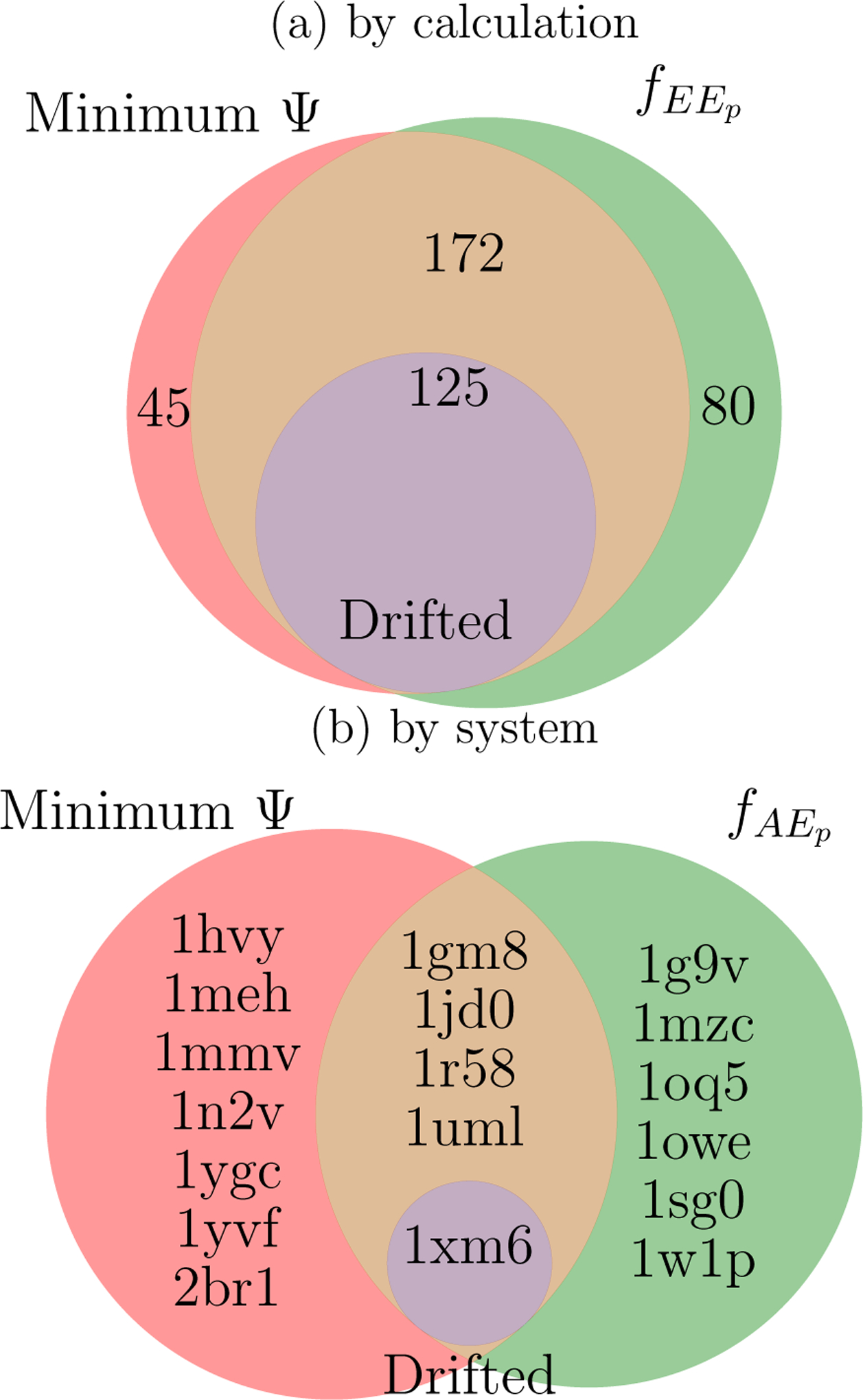
Incorrect binding pose predictions, or geometric decoys, arise when a nonnative pose has a lower score than any native pose. The Venn diagrams show the overlap between sets of (a) BPMF calculations or (b) systems in which there are geometric decoys according to the interaction energy in milestone E (Minimum Ψ), the pose-specific BPMF ($f_{E{E}_p}$ in panel (a) and $f_{A{E}_p}$ in panel (b)), or because no native poses were observed (Drifted). Panel (a) is labeled by the number of BPMF calculations and is based on poses observed in each calculation. Panel (b) is labeled by PDB identifiers for the particular systems and is based on poses observed in all BPMF calculations for a system.

DISCUSSION

Thermodynamic state initialization and automatic adaptation reliably yields reasonable protocols

The selection of intermediate states between two thermodynamic milestones of interest is a ubiquitous problem in molecular simulation. The usual approach to this problem is an iterative trial-and-error process starting from a naive protocol, checking for issues such as replica exchange bottlenecks, and manually inserting and removing states as necessary. I have developed a simple and robust approach to initialize a series of thermodynamic states based on only a single adjustable parameter, the thermodynamic speed. In the vast majority of cases, the initialization protocol yielded consistent replica exchange rates across neighboring thermodynamic states without further fine-tuning. I also developed an automated approach to add additional states when the observed replica exchange rate falls below 40%. With this procedure, I was able to run a large number of simulations on a diverse array of protein-ligand complexes without manual intervention. The described approach to trailblazing and adapting thermodynamic state space may find use in other classes of simulations.

Replica exchange calculations in this present study include more thermodynamic states than most published molecular simulations. Conventional wisdom about replica exchange is that an optimal number of replicas will maximize efficiency. With too few replicas, there is limited configuration space overlap between neighbors and exchange rates are vanishingly small. With too many replicas, metrics of replica exchange efficiency, such as a mean round-trip time, diminish. However, in a recent study involving extensive simulation of several distinct processes, my group found that if there are no bottlenecks in which the replica exchange rate is below 40%, the number of states has little impact on the convergence of free energy estimates³⁵. Hence, I chose to include a large number of states to minimize the probability that later sampling will explore different regions of configuration space and reduce the exchange rate between neighboring states.

While useful, the described thermodynamic state initialization process remains imperfect. Replica exchange is particularly beneficial when the important configuration space of a thermodynamic state is a subset of the important configuration space of another. The present procedure is limited to the variation of a single thermodynamic parameter between milestones. Future improvements could accommodate varying multiple parameters (e.g. separate parameters for the temperature, van der Waals grids, and electrostatic grids) in between thermodynamic states of interest to promote sampling while minimizing unnecessary traversals of configuration space.

Most free energy differences between sampled states are converged

It has been argued that many simulations of biomolecular binding processes do not adequately sample relevant configuration space and therefore results are not converged and are irreproducible⁴³. Within his discussion of problematic degrees of freedom, Mobley⁴³ highlighted ligand binding modes and internal conformational changes in small molecules as common reasons for failed convergence. In the majority of simulations considered in this paper, f_AD estimates are very precise. Achieving precise free energy differences between milestones A and D requires adequate sampling of both of the aforementioned problematic classes of conformational transitions. The precise results suggest that the described approach is successful at addressing the sampling problems for simulated thermodynamic states.

BPMF convergence and native pose prediction is predicated on overlap between milestones D and E

While free energy differences between milestones A and D were precise in nearly all systems, the precision of f_DE estimates was more variable, limiting the convergence of BPMF calculations and the accuracy of native pose prediction. The performance of f_DE estimates and native pose prediction was highly dependent on whether the ligand was considered desolvated or fully solvated when bound to the protein, implicating the solvation option as a key factor in the overlap between the important configuration spaces of milestones D and E. The strong performance of the interaction energy based on milestone E in identifying the native binding pose suggests that it is desirable to bring sampling closer to the importance configuration space of milestone E (opposed to making milestone E more like milestone D with either solvation option). In future work, more precise BPMF estimates may be attained by introducing intermediate states or by altering the force field for milestone D to become more similar to milestone E. For example, milestone D could be based on a grid that uses generalized Born instead of Poisson-Boltzmann electrostatics. A related possibility is to model desolvation of the ligand due to the receptor using a grid-based fractional desolvation term⁴⁴. The strong performance of the consensus binding pose prediction based on all BPMF estimates for a system suggests that more precise BPMF calculations will also yield improved binding pose prediction.

Even with shortcomings in BPMF convergence, the present native pose prediction strategies perform comparably to other docking programs (Table 1). Because the Astex Diverse Set⁹ is a widely used benchmark, I will only mention a few results. In the original paper on the dataset, the standard GOLD protocol predicted the native pose within 2 Å in 80.5% of systems⁹. With best-practice structures, GLIDE was successful according to the same criterion for in 82% of systems (Figure 1 of Repasky et al.⁴⁵). ICM has particularly strong performance, successful in 91% of systems⁴⁶. For comparison, when ranking poses with the free energy based on the force field in milestone E, the calculations described herein are successful in 75.8% of Desolvated and 83.9% of Full BPMF calculations (Table 1). A caveat to this comparison is that the BPMF calculations were started with the native pose (as well as poses generated by UCSF DOCK 6), but other methods were required to sample the binding pose de novo. Another helpful reference point is a recent comprehensive evaluation by Wang et al.⁴⁷, who found that 10 programs were successful in 40% to 60% of complexes in the PDBbind refined set (version 2014).

Ligand electrostatics in the protein environment are better treated as fully solvated

One of the more surprising results is that the Full solvation option outperforms the Desolvated option by yielding lower BPMFs and better binding pose predictions. After all, a ligand that is bound to a protein must shed most if not all of its hydration shell! A possible explanation is that many protein binding sites could mimic the dielectric environment of water. To facilitate protein folding and solubility, soluble proteins usually contain hydrophobic residues in the interior and hydrophilic residues on the exterior. Since binding sites are primarily on protein surfaces, bound ligands may be surrounded by residues whose dielectric behavior resembles water.

CONCLUSIONS

I have developed a reasonably robust method to estimate BPMFs for protein-ligand systems. The largest sources of imprecision are found to be configuration space overlap between representations of the complex.

References

- 1.Minh DDL, J. Chem. Phys 137, 104106 (2012). [DOI] [PMC free article] [PubMed] [Google Scholar]
- 2.Nguyen TH and Minh DDL, J. Chem. Phys 148, 104114 (2018). [DOI] [PMC free article] [PubMed] [Google Scholar]
- 3.Mobley DL, Graves AP, Chodera JD, McReynolds AC, Shoichet BK, and Dill KA, J. Mol. Biol 371, 1118 (2007). [DOI] [PMC free article] [PubMed] [Google Scholar]
- 4.Ucisik MN, Zheng Z, Faver JC, and Merz KM, J. Chem. Theory Comput 10, 1314 (2014). [DOI] [PMC free article] [PubMed] [Google Scholar]
- 5.Xie B, Nguyen TH, and Minh DDL, J. Chem. Theory Comput 13, 2930 (2017). [DOI] [PMC free article] [PubMed] [Google Scholar]
- 6.Nguyen TH, Zhou H-X, and Minh DDL, J. Comput. Chem 39, 621 (2018). [DOI] [PMC free article] [PubMed] [Google Scholar]
- 7.Minh DDL, arXiv 1507.03703v1 (2015).
- 8.Xie B and Minh DDL, J. Comput.-Aided Mol. Des 33, 61 (2019). [DOI] [PMC free article] [PubMed] [Google Scholar]
- 9.Hartshorn MJ, Verdonk ML, Chessari G, Brewerton SC, Mooij WTM, Mortenson PN, and Murray CW, J. Med. Chem 50, 726 (2007). [DOI] [PubMed] [Google Scholar]
- 10.Gallicchio E and Levy RM, J. Comput.-Aided Mol. Des 26, 505 (2012). [DOI] [PMC free article] [PubMed] [Google Scholar]
- 11.Wang K, Chodera JD, Yang Y, and Shirts MR, J. Comput.-Aided Mol. Des 27, 989 (2013). [DOI] [PMC free article] [PubMed] [Google Scholar]
- 12.Wang L, Wu Y, Deng Y, Kim B, Pierce L, Krilov G, Lupyan D, Robinson S, Dahlgren MK, Greenwood J, et al. , J. Am. Chem. Soc 137, 2695 (2015). [DOI] [PubMed] [Google Scholar]
- 13.Pattabiraman N, Levitt M, Ferrin TE, and Langridge R, J. Comput. Chem 6, 432 (1985). [Google Scholar]
- 14.Meng EC, Shoichet BK, and Kuntz ID, J. Comput. Chem 13, 505 (1992). [Google Scholar]
- 15.Minh DDL, J. Comput. Chem 39, 1200 (2018). [DOI] [PMC free article] [PubMed] [Google Scholar]
- 16.Hinsen K, J. Comput. Chem 21, 79 (2000). [Google Scholar]
- 17.Shirts MR and Chodera JD, J. Chem. Phys 129, 124105 (2008). [DOI] [PMC free article] [PubMed] [Google Scholar]
- 18.Wang J, Wolf RM, Caldwell JW, Kollman PA, and Case DA, J. Comput. Chem 25, 1157 (2004). [DOI] [PubMed] [Google Scholar]
- 19.Jakalian A, Bush BL, Jack DB, and Bayly CI, J. Comput. Chem 21, 132 (1999). [DOI] [PubMed] [Google Scholar]
- 20.Jakalian A, Jack DB, and Bayly CI, J. Comput. Chem 23, 1623 (2002). [DOI] [PubMed] [Google Scholar]
- 21.Eastman P and Pande VS, Comput. Sci. Eng 12, 34 (2010). [DOI] [PMC free article] [PubMed] [Google Scholar]
- 22.Onufriev A, Bashford D, and Case DA, Proteins: Struct., Funct., Bioinf 55, 383 (2004). [DOI] [PubMed] [Google Scholar]
- 23.Baker NA, Sept D, Joseph S, Holst MJ, and McCammon JA, Proc. Natl. Acad. Sci. USA 98, 10037 (2001). [DOI] [PMC free article] [PubMed] [Google Scholar]
- 24.Oberlin D and Scheraga HA, J. Comput. Chem 19, 71 (1998). [Google Scholar]
- 25.Venkatachalam CM, Jiang X, Oldfield T, and Waldman M, J. Mol. Graph. Model 21, 289 (2003). [DOI] [PubMed] [Google Scholar]
- 26.Diller DJ and Verlinde CLMJ, J. Comput. Chem 20, 1740 (1999). [Google Scholar]
- 27.Michel J and Essex JW, J. Comput.-Aided Mol. Des 24, 639 (2010). [DOI] [PubMed] [Google Scholar]
- 28.Duane S, Kennedy AD, Pendleton BJ, and Roweth D, Phys. Lett. B 195, 216 (1987). [Google Scholar]
- 29.Jiang W and Roux B, J. Chem. Theory Comput 6, 2559 (2010). [DOI] [PMC free article] [PubMed] [Google Scholar]
- 30.Chodera JD and Shirts MR, J. Chem. Phys 135, 194110 (2011). [DOI] [PubMed] [Google Scholar]
- 31.Lu N and Kofke DA, J. Chem. Phys 114, 7303 (2001). [Google Scholar]
- 32.Weinhold F, J. Chem. Phys 63, 2479 (1975). [Google Scholar]
- 33.Shenfeld DK, Xu H, Eastwood MP, Dror RO, and Shaw DE, Phys. Rev. E 80, 46705 (2009). [DOI] [PubMed] [Google Scholar]
- 34.Crooks GE, Phys. Rev. Lett 99, 100602 (2007). [DOI] [PubMed] [Google Scholar]
- 35.Nguyen TH and Minh DDL, J. Chem. Theory Comput 12, 2154 (2016). [DOI] [PubMed] [Google Scholar]
- 36.Chodera JD, Chem J. Theory Comput 12, 1799 (2016). [DOI] [PMC free article] [PubMed] [Google Scholar]
- 37.Zwanzig R, J. Chem. Phys 22, 1420 (1954). [Google Scholar]
- 38.van der Walt S, Colbert SC, and Varoquaux G, Comput. Sci. Eng 13, 22 (2011). [Google Scholar]
- 39.Lang P, Brozell SR, Mukherjee S, Pettersen E, Meng EC, Thomas V, Rizzo RC, Case DA, James T, and Kuntz ID, RNA 15, 1219 (2009). [DOI] [PMC free article] [PubMed] [Google Scholar]
- 40.Pordes R, Petravick D, Kramer B, Olson D, Livny M, Roy A, Avery P, Blackburn K, Wenaus T, Wu¨rthwein F, et al. , J. Phys.: Conf. Ser 78, 012057 (2007). [Google Scholar]
- 41.Towns J, Cockerill T, Dahan M, Foster I, Gaither K, Grimshaw A, Hazlewood V, Lathrop S, Lifka D, Peterson GD, et al. , Comput. Sci. Eng 16, 62 (Sep-Oct 2014). [Google Scholar]
- 42.Wood RH, Muhlbauer WCF, Thompson PT, Mühlbauer WC, and Thompson PT, J. Phys. Chem 95, 6670 (1991). [Google Scholar]
- 43.Mobley DL, J. Comput.-Aided Mol. Des 26, 93 (2012). [DOI] [PubMed] [Google Scholar]
- 44.Mysinger MM and Shoichet BK, J. Chem. Inf. Model 50, 1561 (2010). [DOI] [PubMed] [Google Scholar]
- 45.Repasky MP, Murphy RB, Banks JL, Greenwood JR, Tubert-Brohman I, Bhat S, and Friesner RA, J. Comput.-Aided Mol. Des 26, 787 (2012). [DOI] [PubMed] [Google Scholar]
- 46.Neves M. a. C., Totrov M, and Abagyan RA, J. Comput.-Aided Mol. Des 26, 675 (2012). [DOI] [PMC free article] [PubMed] [Google Scholar]
- 47.Wang Z, Sun H, Yao X, Li D, Xu L, Li Y, Tian S, and Hou T, Phys. Chem. Chem. Phys 18, 12964 (2016). [DOI] [PubMed] [Google Scholar]
- 48.Sfiligoi I, Bradley DC, Holzman B, Mhashilkar P, Padhi S, and Wurthwein F, in 2009 WRI World Congress on Computer Science and Information Engineering (IEEE, Los Angeles, California USA, 2009), pp. 428–432, ISBN 978-0-7695-3507-4. [Google Scholar]
- 49.Humphrey W, Dalke A, and Schulten K, J. Mol. Graphics 14, 33 (1996). [DOI] [PubMed] [Google Scholar]
Associated Data
This section collects any data citations, data availability statements, or supplementary materials included in this article.