CALDER: Inferring phylogenetic trees from longitudinal tumor samples

Abstract

Summary

Longitudinal DNA sequencing of cancer patients yields insight into how tumors evolve over time or in response to treatment. However, sequencing data from bulk tumor samples often has considerable ambiguity in clonal composition complicating the inference of ancestral relationships between clones. We introduce CALDER, an algorithm to infer phylogenetic trees from longitudinal bulk DNA sequencing data. CALDER explicitly models a longitudinally-observed phylogeny incorporating constraints that longitudinal sampling imposes on phylogeny reconstruction. We show on simulated bulk tumor data that longitudinal constraints substantially reduce ambiguity in phylogeny reconstruction and that CALDER outperforms existing methods that do not leverage this longitudinal information. On real data from two chronic lymphocytic leukemia patients, we find that CALDER reconstructs more plausible and parsimonious phylogenies than existing methods, with CALDER phylogenies containing fewer tumor clones per sample. CALDER’s use of longitudinal information will be advantageous in further studies of tumor heterogeneity and evolution.

Primer

Cancer is an evolutionary process where somatic mutations accumulate in a population of cells over time. The population of cells that form a tumor is heterogeneous, with subpopulations of cells, or clones, containing different complements of somatic mutations. The abundances of clones change over time and in response to treatment, due to selection for advantageous mutations and/or random genetic drift. To study the forces that shape tumor evolution, cancer researchers use DNA sequencing of one or more samples from the same tumor to measure the genomic heterogeneity within a tumor. Researchers then employ techniques from phylogenetics to reconstruct the somatic mutational history of individual tumors.

A major challenge in phylogenetic analysis of cancer is that the vast majority of cancer sequencing uses DNA from bulk tumor samples; thus, the resulting data is a mixture of DNA sequences from cancerous cells with different somatic mutations, as well as from normal cells. Since standard phylogenetic techniques are not designed to handle such mixtures, a number of specialized phylogenetic mixture algorithms have been developed in the past few years. These specialized algorithms derive the composition of each tumor sample as a mixture of clones and infer the ancestral relationships between these clones. While phylogenetic mixture algorithms are computationally sophisticated, it is often impossible to derive a unique clonal structure and phylogenetic tree from bulk tumor data: there are too many ways to separate the mixed data into clones.

A promising approach to overcome the ambiguity in bulk tumor sequencing data is to identify additional structure in the data. For example, in some cases, multiple tumor samples are sequenced longitudinally, i.e., at multiple distinct times during the progression of cancer in an individual. The issue of separating the mixed DNA data in each individual bulk tumor sample persists in longitudinal sequencing. However, the temporal ordering of longitudinal samples provides additional information that reduces ambiguity in the inference of clonal composition and the reconstruction of a phylogenetic tree. In this paper, we show how to leverage this temporal information to derive more accurate phylogenetic trees from longitudinal bulk tumor samples. We introduce a new algorithm, Cancer Analysis of Longitudinal Data through Evolutionary Reconstruction (CALDER), that models the structure in longitudinal samples. We show that CALDER outperforms existing phylogenetic mixture algorithms that do not utilize temporal relationships between samples.

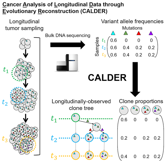
Graphical Abstract

eTOC Blurb:

Cancer is an evolutionary process in which genetically distinct populations of cells accumulate somatic mutations. Reconstructing this evolutionary process from bulk tumor samples is challenging, as such samples are mixtures of multiple subpopulations, or clones. We introduce Cancer Analysis of Longitudinal Data through Evolutionary Reconstruction (CALDER), an algorithm to reconstruct tumor phylogenies from longitudinal bulk DNA sequencing data by leveraging the temporal relationships between longitudinal samples. CALDER outperforms existing approaches that do not utilize temporal information.

Introduction

Cancer is an evolutionary process, where cells accumulate somatic mutations over time (Nowell 1976). As a result of this clonal evolution, most tumors are heterogeneous, with populations of cells, or clones, containing different combinations of somatic mutations. The clonal composition of a tumor may shift over time, particularly in response to treatment. Longitudinal sequencing, or sequencing DNA from tumor samples of the same patient at different time-points, is increasingly being used to track the progression of cancer over time (M. Griffith et al. 2015; Nadeu et al. 2016; Rose-Zerilli et al. 2016; Haber and Velculescu 2014). For example, Nadeu et al. (2016) performed longitudinal DNA sequencing of 48 chronic lymphocytic leukemia (CLL) patients to study the impact of clonal and subclonal driver mutations on clonal dynamics and disease progression. In another study, M. Griffith et al. (2015) performed longitudinal sequencing of an acute myeloid leukemia (AML) patient and found a clone with a driver mutation in the gene IDH2 that was present in less than 2% of the pretreatment sample, but subsequently became the dominant clone after relapse. Longitudinal sequencing helps to measure clones that are present in small proportions prior to treatment, but become founder clones of a relapse or metastasis. Early longitudinal sequencing studies were mostly performed in blood cancers where sample acquisition is straightforward. With the advent of noninvasive sampling of circulating tumor DNA (ctDNA) and circulating tumor cells (CTCs) – i.e., liquid biopsies (Haber and Velculescu 2014) – longitudinal sequencing is now possible for many types of cancer. Longitudinal sequencing studies allow researchers to track the evolutionary trajectories of cancer and hold promise for providing greater understanding of how tumor clones and individual mutations interact and respond to treatment.

A fundamental step in studying the evolutionary dynamics of cancer is the construction of a phylogenetic tree that describes the ancestral history of somatic mutations and cell lineage. The vertices of such a tree correspond to cells (or clones) in the tumor, and edges describe ancestral relationships between cells/clones. The problem of constructing a phylogenetic tree from measurements of individual taxa is a well-studied problem. However, when analyzing DNA sequencing data of bulk tumor samples – each containing thousands to millions of cells – one must instead build a phylogenetic tree from mixtures of taxa. In recent years, a number of specialized algorithms have been developed to solve this phylogenetic mixture problem (Strino et al. 2013; Jiao et al. 2014; El-Kebir, Oesper, et al. 2015; Popic et al. 2015; Malikic et al. 2015; Deshwar et al. 2015; El-Kebir, Satas, Oesper, et al. 2016; Satas and Raphael 2017; H. Dang et al. 2017; Jiang et al. 2016; Reiter et al. 2017; El-Kebir, Satas, and Raphael 2018). While these algorithms are designed to address the complexities of bulk sequencing data, none directly integrate the constraint that samples are measured longitudinally.

In this paper, we introduce an algorithm, Cancer Analysis of Longitudinal Data through Evolutionary Reconstruction (CALDER), that leverages information in longitudinal samples to reconstruct phylogenetic trees from longitudinal bulk DNA sequencing data. CALDER relies on a model of longitudinally-observed phylogenies as vertex-colored trees where the order of colors encodes the temporal order of the samples. We formulate the Longitudinal Variant Allele Frequency Factorization Problem (LVAFFP), a generalization of the problem of reconstructing a tree from bulk samples where the samples are temporally ordered. We derive a combinatorial characterization of the solutions to the LVAFFP as constrained spanning trees of a directed graph constructed from the variant allele frequencies (VAFs) of somatic mutations. Based on insights on the longitudinal structure of DNA sequencing data, we also develop an absence-aware method to cluster mutations into clones. We compare CALDER to several existing approaches (Jiao et al. 2014; El-Kebir, Oesper, et al. 2015; Malikic et al. 2015) for tumor phylogeny reconstruction on simulated and real longitudinal sequencing data. On simulated bulk sequencing data, we show that longitudinal constraints reduce the number of phylogenetic trees that describe the data by up to 90%, and on average by 30%. On real data from chronic lymphocytic patients (Rose-Zerilli et al. 2016; Schuh et al. 2012), we find that CALDER produces more plausible evolutionary trees that respect the longitudinal ordering of the data.

Results

CALDER algorithm

In this section, we describe our CALDER algorithm that infers a clone tree and the clonal composition of a tumor from longitudinal bulk DNA sequencing data. First, we introduce a model for longitudinally-observed phylogenies as vertex-colored trees in which the order of colors encodes the temporal order of the samples. Next, we formulate the Longitudinal Variant Allele Frequency Factorization Problem (LVAFFP), a generalization of the problem of reconstructing a tree from bulk samples where the samples are temporally ordered. Finally, we describe how to model uncertainty in observed mutation frequencies using an absence-aware clustering algorithm and formulate the LVAFFP with uncertainty.

Longitudinal observations of tumor evolution

We represent the evolutionary history of a tumor at the single-cell level as an edge-weighted binary cell tree P = (V,E), where a vertex v ∈ V is a cell, a directed edge (v, w) ∈ E between two cells indicates a parental relationship, the weight of an edge indicates the lifespan of a cell, and edges are labeled by the mutation(s) that distinguish child from parent. In longitudinal data, we observe a cell tree at a series of time-points t₁ < t₂ <… < t_m during the evolutionary process. Let C₁,…, C_m be the disjoint sets of cells present at time-points t₁,…t_m, respectively. We define a longitudinally-observed cell tree P = (V, E, c) to be a vertex-colored tree where:

1. Every vertex v ∈ V has a color c(v) ∈ {0,…, m} where c(v) = i indicates that v ∈ C_i, and c(v) = 0 indicates that v is not observed;

2. For every path p = r,…, v from the root r to a leaf v, the non-zero colors on the path are encountered in numerical order.

Figure 1A shows an example of a longitudinally-observed cell tree.

Figure 1:

(A) (Left) A cell tree describes the cell division and mutation history of a tumor, where vertices are cells and edges are parental relationships. We are typically not able to observe this evolutionary process continuously, and instead have a set of observations from discrete time-points t₁, t₂, and t₃. (Right) A longitudinally-observed cell tree describes the ancestral relationships between the observed cells. Cells are labeled (colored) with the time-point that they are observed. (B) (Left) A clone proportion matrix U describes the composition of a tumor at each time-point t_i, and a perfect phylogeny matrix B (1-to-1 with a mutation tree T) describes the evolutionary relationships between clones. (Right) Construction of the observed clone tree P_U,B from clone proportion matrix U and perfect phylogeny matrix B.. (C) Not all VAFFP solutions correspond to longitudinally-observed clone trees. In this example, the frequency matrix F has multiple factorizations. One factorization F = U₁B₁ (top) corresponds to a longitudinally-observed clone tree, but another factorization F = U₂B₂ (bottom) does not. This is evident in the red highlighted path, which does not respect the ordered coloring.

With bulk sequencing data, we do not observe individual cells directly and instead reconstruct tumor evolution at the resolution of clones, or populations of cells that share a set of mutations. We define a longitudinally-observed clone tree P = (V,E,c) where each vertex v ∈ V corresponds to a distinct population of cells, edges (v, w) ∈ E are ancestral relationships, and colors c follow the properties stated above.

Reconstructing longitudinal phylogenetic trees from bulk sequencing data

We first describe the problem of constructing a phylogenetic tree from n single-nucleotide mutations measured in m bulk tumor samples from the same individual. For each sample t and each mutation i, we compute the variant allele frequency (VAF) f_t,i as the fraction of reads from sample t that cover position i and contain the variant allele (i.e., a somatic mutation) at position i. In the absence of copynumber aberrations, the VAF f_t,i is directly proportional to the proportion of cells in sample t that contain mutation i. We represent the observed data as an m × n frequency matrix F =[f_t,i]. As in El-Kebir, Oesper, et al. (2015), we assume that each mutation corresponds to a clone (i.e., we assume that mutations have been clustered according to their VAFs (Roth et al. 2014; Miller et al. 2014; Jiao et al. 2014). Each tumor sample t is then a mixture of clones, where u_t,v is the proportion of clone v in sample t. Thus, u_t,v≥0 and ${\sum }_{v=1}^n{u}_{t,v}\le 1$. We define the m×n clone proportion matrix U = [u_t,v].

The fundamental problem in reconstructing a phylogenetic tree from bulk tumor samples is to identify the clone tree T and clone proportion matrix U that generated the observed mutation frequencies F. Multiple algorithms have been developed to solve this problem in various settings (Jiao et al. 2014; El-Kebir, Oesper, et al. 2015; Malikic et al. 2015; Popic et al. 2015; Deshwar et al. 2015; Satas and Raphael 2017; El-Kebir, Satas, Oesper, et al. 2016; H. Dang et al. 2017; El-Kebir, Satas, and Raphael 2018; Jiang et al. 2016; Reiter et al. 2017). All of these algorithms rely on the infinite sites assumption, (ISA), which states that a mutation occurs at a genomic position at most once during evolution. Under the ISA – also known as the perfect phylogeny model (Gusfield 1997) – there is a one-to-one correspondence between phylogenetic trees T and a collection of 0 / 1-valued perfect phylogeny matrices B whose rows correspond to clones and columns correspond to mutations, where b_v,i indicates if clone v has mutation i.

Using this one-to-one correspondence, El-Kebir, Oesper, et al. (2015) formulated the problem of reconstructing a phylogenetic tree from bulk tumor samples as a matrix factorization problem.

Variant Allele Frequency Factorization Problem (VAFFP).

Given frequency matrix F, find perfect phylogeny matrix B and clone proportion matrix U such that F = UB.

In the VAFFP, there are no assumptions regarding the temporal relationships between bulk sequencing samples. Indeed, often there are multiple factorizations F = UB for a given frequency matrix F. Suppose now that the DNA sequencing data is obtained from longitudinal sampling of bulk tumor samples at a series of time-points t₁ < t₂ < …t_m. Intuitively, the information that samples are longitudinal should provide additional constraints on the phylogenetic tree T (or equivalently matrix B) and the clone proportions U. We now derive these constraints. First, we recall that the mutation trees T =(V_T, E_T) describe the evolutionary relationships between clones. Vertices v ∈ V_T correspond to clones, and edges (v, w) ∈ E_T correspond to parental relationships between clones. We label each edge of a mutation tree with the mutation(s) that distinguish the parent and child vertex. Let M_v be the set of mutations present in the clone corresponding to vertex v. Edge (v,w) ∈ E_T is labeled by the difference M_v \ M_w in mutations between the clones. Under the ISA, each mutation appears at most once on an edge in T. Let μ be a mapping from each vertex v ∈ V_T to the mutation on its incoming edge, e.g., μ (v) = j . Without loss of generality, we use a single phylogenetic character to represent the set of mutations on each edge. Mutation trees are analogous to n-clonal trees as described by El-Kebir, Oesper, et al. (2015). Under the ISA, the clones that contain the mutation i are the first clone v that acquired mutation i (i.e., μ (v) = i ), and the descendants Δ_v of v. Thus, we have that the frequency $f_{t,i}={\sum }_{w=1}^n{u}_{t,w}{b}_{w,i}=u_{t,v}+{\sum }_{w\in {\Delta }_v}{u}_{t,w}$.

The constraints provided by longitudinal samples are derived on a vertex-colored observed clone tree P_U,B, which is determined by the clone proportion matrix U and perfect phylogeny matrix B (together with B’s corresponding mutation tree T). Figure 1B gives an example of the construction of P_U,B, with further details in STAR Methods. The colored vertices in P_U,B correspond to non-zero entries in U, and the edges in P_U,B maintain the ancestral relationships in T: if mutation i precedes mutation j in T, then i also precedes j in P. In general, there are multiple clone trees that could be generated from a U and B – for example, one could add arbitrarily many unobserved clones with corresponding uncolored vertices. However, this construction yields a unique clone tree P_U,B. Moreover, if there exists a longitudinally-observed clone tree corresponding to the factorization (U, B), then the P_U,B constructed as described in STAR Methods is longitudinally observed.

Thus, given DNA sequencing data from longitudinal bulk tumor samples, the problem one wants to solve is the following variation of the VAFFP.

Longitudinal Variant Allele Frequency Factorization Problem (LVAFFP).

Given frequency matrix F whose rows correspond to longitudinal samples, find a perfect phylogeny matrix B and clone proportion matrix U such that F = UB and the observed clone tree P_U,B is longitudinally observed. Interestingly, given a frequency matrix F obtained from longitudinal sampling, it is possible to obtain a factorization F = UB where the observed clone tree P_U,B is not longitudinally observed (Figure 1C). Thus, the LVAFFP is not equivalent to the VAFFP. Moreover, the LVAFFP, like the VAFFP, is NP-complete (see proof in Method S1). We characterize solutions to the LVAFFP in STAR Methods and describe both an ILP and an enumeration algorithm to solve the LVAFFP in Method S1.

Reconstructing longitudinal trees with uncertain data

In the previous sections, we assumed that the observed mutation frequencies F were the true mutation frequencies. On real data, the mutation frequencies are estimated from counts of aligned sequence reads and thus the mutation frequencies have uncertainty. This uncertainty limits the resolution of tumor subpopulations that can be distinguished, and the standard approach is to cluster mutations and infer the phylogeny on these clusters (Roth et al. 2014; Miller et al. 2014; Zare et al. 2014). Indeed, we have observed that popular mutation clustering algorithms do not explicitly distinguish between mutations that are present at very small frequencies in a sample and mutations that are absent (Roth et al. 2014; Miller et al. 2014). This is particularly problematic in the context of the LVAFFP because the coloring of the observed clone tree P_U,B depends on the presence and absence of clones in samples. As the inferred clones depend directly on the mutation clustering, a clustering error could invalidate the correct longitudinal solution.

We address this issue in the context of the LVAFFP by introducing an absence-aware clustering algorithm that explicitly models the presence or absence of mutations in a sample. This algorithm relies on the principle that if a pair of mutations is present in the same set of clones, then the pair will be present in the same set of samples. We leverage this information to distinguish between true low-frequency mutations and absent mutations by partitioning the set of mutations into subsets of cooccurring mutations prior to clustering (see STAR Methods for details).

Even with the correct clustering of mutations, there remains ambiguity in the solution of the LVAFFP. Specifically, given an uncertain frequency matrix F (on individual mutations or clusters of mutations), we aim to find an $\widehat{F}\approx F$ such that $\widehat{F}=UB$ where the observed clone tree P_U,B is longitudinally observed. However, for a fixed mutation tree T (with corresponding perfect phylogeny matrix B), there may be many possible clone proportion matrices U such that F ≈ UB and P_U,B is longitudinally observed. In particular, it is generally possible to infer a U with all entries strictly positive and many entries having small values. These trivially longitudinal solutions are typically uninteresting, as they imply that all clones are present at all time-points even through the inferred clonal proportions are very small in many samples (see STAR Methods for details). We aim to find longitudinal solutions (U, B) where the clones present in each sample are strongly supported by the observed frequencies. To address this, we impose two additional constraints on our solutions. First, we minimize the number of non-zero entries in U by adding a regularization term ∥U∥₀ to the objective function. Second, we require that all non-zero entries of U exceed a minimum threshold h; that is, we require that u_t,v = 0 or u_t,v ≥ h for all t, v. These additional constraints prevent trivially longitudinal solutions and require that small clone proportions are well supported by the data.

To model uncertainty in VAFs during tree reconstruction, we use confidence intervals as was done previously (Strino et al. 2013; El-Kebir, Oesper, et al. 2015; Popic et al. 2015; El-Kebir, Satas, Oesper, et al. 2016; Malikic et al. 2015). Extending longitudinal constraints to using generative probabilistic models of observed read counts (Jiao et al. 2014; Satas and Raphael 2017; Deshwar et al. 2015) is left for future work. Specifically, we derive a confidence interval $f_{t,i}^{-}\le f_{t,i}\le f_{t,i}^{+}$ for each entry f_t,i from the number of reads covering position i. Let F⁻ be the matrix of lower bounds on frequency values, and let F⁺ be the matrix of upper bounds. Using these confidence intervals, we formulate the following problem.

Longitudinal Variant Allele Frequency Factorization Problem with Uncertainty (LVAFFP-U).

Given frequency matrices F⁻ and F⁺, find a frequency matrix $\widehat{F}$, clone proportion matrix U, and perfect phylogeny matrix B such that: $\widehat{F}=UB$, $f_{t,i}^{-}\le {\widehat{f}}_{t,i}\le f_{t,i}^{+}$ for all time-points t and mutation clusters i, u_t,v ∉ (0, h) for all time-points t and clones v, ∥U∥₀ is as small as possible, and P_U,B is longitudinally observed.

Our algorithm, Cancer Analysis of Longitudinal Data through Evolutionary Reconstruction (CALDER) formulates and solves this problem as a mixed integer linear program (MILP) (see Method S1).

Longitudinal constraints reduce ambiguity on simulated data

First, we use simulated data to assess what fraction of solutions to the VAFFP are longitudinal, i.e., solutions to the LVAFFP. We generate 10 mutation trees using the simulation procedure described in El-Kebir, Satas, and Raphael (2018), each tree having between 4 and 13 vertices. For each tree, we generate 10⁶ frequency matrices F for each value m = 2,…,9 samples, resulting in a total of 8×10⁷ F matrices. Further details are in STAR Methods. We solve the VAFFP and the LVAFFP for each F, counting the number $S={\mathcal{S}}_F$ of solutions to the VAFFP and the number $L={\mathcal{L}}_F$ of solutions to the LVAFFP. Note that because all solutions to the LVAFFP are also solutions to the VAFFP, L ≥ S. Because we are primarily interested in the difference between L and S, we restrict our analysis to those instances for which L < S. We find that on the 423,328 instances with L < S (representing 0.5%-11% of the instances for each tree; mean 5.3%, median 3.9%), L ≈ 0.7S on average (and also median), with a minimum of L ≈ 0.07S (Figure 2A-B). These results demonstrate that even with no error in the VAFs, longitudinal constraints result in fewer possible solutions to the VAFFP in a nontrivial fraction of cases.

Figure 2: Comparisons on simulated data.

(A-B) Comparison of the number S of solutions to the VAFFP and the number L of solutions to the LVAFFP on 423,328 simulated m×n frequency matrices F which were generated uniformly at random from a total of 10 tree topologies, with m = 2,…, 9 and n = 4,…,13 . (A) Histogram showing the proportion of solutions to the VAFFP which are also solutions to the LVAFFP. (B) Scatterplot showing how the relationship between S and L. Note that we exclude instances where L = S. (C-D) Results from CALDER, PhyloWGS, and CITUP on 178 simulated tumors. (C) The tree error (proportion of ancestor-descendant relationships incorrectly inferred) for each method on each tumor. (D) The presence-absence error for each method on each tumor.

CALDER accurately recovers tumor evolution on simulated data

We compare CALDER with two existing methods for phylogenetic tree reconstruction on simulated bulk DNA sequencing data. We simulate data using the tumor simulation from El-Kebir, Satas, and Raphael (2018) modified to model longitudinal sampling (see STAR Methods for details). We generated 178 simulated tumors using this model, each with 2-5 longitudinal samples (mean 4.97, median 5) and 65-234 mutations (mean 129.33, median 126). We ran CALDER, PhyloWGS (Deshwar et al. 2015) and CITUP (Malikic et al. 2015) on each collection of simulated tumor samples using the default parameters for each method (see STAR Methods and Table S1 for running time and space details). For CALDER we first cluster mutations using the absence-aware clustering algorithm described in STAR Methods, while for PhyloWGS and CITUP we use their built-in clustering methods. We assess the performance of each algorithm using two metrics: (1) tree error, the proportion of inferred ancestor-descendant relationships that are incorrect; (2) presence-absence error, the proportion of mutations that are incorrectly inferred as present (mutation frequency > 0) or absent (mutation frequency = 0). We describe the computation of these quantities in STAR Methods.

We find that CALDER infers significantly more accurate trees than other methods, with a median tree error of 0.269, as opposed to 0.297 for PhyloWGS and 0.552 for CITUP (Figure 2C; CALDER vs. PhyloWGS p < 10⁻³, CALDER vs. CITUP p < 10⁻³⁰, Wilcoxon signed-rank test). Additionally, CALDER outperforms PhyloWGS and CITUP in the estimation of mutation frequencies F, with a median presence-absence error of 0.199 for CALDER vs. 0.294 for both PhyloWGS and CITUP (Figure 2D; CALDER vs. PhyloWGS p < 10⁻²⁹. CALDER vs. CITUP p < 10⁻²⁹. Wilcoxon signed-rank test). The similarity between CITUP and PhyloWGS error values is due to the fact that both of them produce trivially longitudinal solutions for nearly all 178 simulated tumors: 170 CITUP solutions are trivially longitudinal (with 4 other solutions violating the permenant extinction condition), and all 178 PhyloWGS solutions are trivially longitudinal. Since mutation frequencies determine clonal proportions, these results imply that CALDER better estimates tumor composition across the time-points compared to PhyloWGS and CITUP.

CALDER analysis of longitudinal CLL sequencing data

We apply CALDER to longitudinal sequencing data from 13 chronic lymphocytic leukemia (CLL) patients from Rose-Zerilli et al. (2016). We find that longitudinal constraints result in fewer phylogenetic trees (i.e., L < S) for 4 of the 7 patients that were sampled at more than 2 time-points, Figure 3 summarizes CALDER results on patient 9, whose tumor was sequenced at 4 time-points during treatment, using targeted deep sequencing of 21 mutations that were identified at diagnosis. CALDER finds 110 maximal mutation trees with 9 mutations, 74 of which yielded longitudinally-observed clone trees (Figure 3A). Figure 3B shows an example mutation tree T₁ and the corresponding longitudinally-observed clone tree P₁.

Figure 3: Longitudinal constraints reduce ambiguity on real data.

CALDER results on CLL patient 9 from Rose-Zerilli et al. Rose-Zerilli et al. (Rose-Zerilli et al. 2016). (A) 110 mutation trees are consistent with the mutation frequencies measured in this patient, but only 74 of these trees correspond to longitudinally-observed clone trees. (B) Example of a mutation tree T₁ and its corresponding longitudinally-observed clone tree P₁. (C) A mutation tree T₂ that does not correspond to a longitudinally-observed clone tree. Without the requirement of a minimum clone proportion h, we obtain the longitudinally-observed clone tree P₂. (D) Clone proportion matrix U₂ corresponding to T₂ has many small entries u_t,v < 0.001 (highlighted in red). These small proportions are required to meet longitudinal constraints. The support for the presence of clone 5 at each time-point t is the difference in frequency between mutations TSPEAR and SERPINB2. With the exception of t₄, this difference is within the confidence bounds of each mutation, and thus clone 5 is unlikely to be present at time-points t₁, t₂, and t₃.

To demonstrate the importance of the regularization term ∥U∥₀ and the minimum clone proportion h in the LVAFFP-U, we examine in more detail a mutation tree T₂ for which CALDER did not report a longitudinally-observed clone tree. We compute a clone proportion matrix U₂ and a mutation tree T₂ that minimize $\mid \widehat{F}-\overline{F}{\mid }_1$, where the entries of $\overline{F}$ are means of the mutation frequency confidence intervals, such that $\widehat{F}=U_2{B}_2$ and the corresponding clone tree P₂ is longitudinally observed. Figure 3C shows the mutation tree T₂ and the corresponding longitudinally-observed clone tree found by this approach. This resulting clone proportion matrix U₂ has many entries u_t,v < 0.001 (Figure 3). In particular, clone 5 is inferred to be present at all time-points in order to meet longitudinal constraints, but has small mixture proportions (< 0.001) at time-points t₂ and t₃ (Figure 3D). According to the structure of the tree T₂, the mixture proportion of clone 5 in a sample is equal to the difference in frequencies between mutations TSPEAR and SERPINB2. While the frequencies of these mutations are well separated at t₄, they are indistinguishable (within the confidence intervals) at t₂ and t₃. Thus, the sequencing data does not support the presence of these clones, implying that the tree T₂ is implausible. This example demonstrates how CALDER leverages longitudinal constraints to reduce ambiguity in the inference of clone trees and clonal composition.

CALDER infers more plausible trees on longitudinal data than existing methods

We apply CALDER to a CLL patient CLL003 from Schuh et al. (2012) that was previously analyzed in the papers introducing the PhyloSub (Jiao et al. 2014), CITUP (Malikic et al. 2015), and AncesTree (El-Kebir, Oesper, et al. 2015) tumor phylogeny algorithms. For this patient, high-depth targeted sequencing was performed at five time-points, and the published analysis reported 20 mutations. We excluded 3 mutations whose VAFs were ≫ 0.5 as these likely overlap with copynumber aberrations; the published results from AncesTree (El-Kebir, Oesper, et al. 2015) also exclude the same 3 mutations. We cluster mutations as described in STAR Methods, obtaining 4 mutation clusters which we label A, B, C, and D. CALDER infers a clone tree containing 4/5 clusters and 15/17 mutations (Figure 4A). This clone tree is longitudinally observed and shows a process of ongoing clonal evolution in this patient, with mutations in cluster B occurring between t₁ and t₂, and mutations in cluster C occurring between t₂ and t₃ We see the tumor composition change from consisting primarily of clone 4 (containing mutation clusters A and D) at t₁, to consisting primarily of clone 3 (containing mutation clusters A, B and C) at t₅.

Figure 4: Results from (A) CALDER and previously published results from (B) PhyloSub (Jiao et al. 2014), (C) AncesTree(El-Kebir, Oesper, et al. 2015), and (D) CITUP(Malikic et al. 2015), on CLL patient CLL003 from Schuh et al. (Schuh et al. 2012).

For CALDER, PhyloSub, and CITUP, edges are labeled by mutation clusters. Mutations that CALDER and AncesTree excluded from tree construction are marked in boldface. Clone proportions are visualized using TimeScape (Smith et al. 2017).

We compare the CALDER solution to the published results from PhyloSub (Jiao et al. 2014), AncesTree (El-Kebir, Oesper, et al. 2015), and CITUP (Malikic et al. 2015) on this patient (Figure 4B-D). The maximum-likelihood tree inferred by PhyloSub (Figure 4B) violates longitudinal constraints (highlighted in red on the tree), with clone 1 being present only at t₂ and t₅. The tree reported by AncesTree (Figure 4B) includes only 5/17 mutations. The corresponding clone tree is trivially longitudinal, with all clones present at all time-points, and consequently implies that the evolution of these clones occurred before the first sample was taken. Many entries in the corresponding clone proportion matrix are very small (highlighted in red), and the presence of these clones is not well-supported by the data. For example, the presence of clone 3 at time-point t₁ is determined by the presence of mutation NPY. However, only 0.09% of the total reads (42 of 45,586) at this locus support this mutation, which is within the range of the estimated per-base sequencing error rate for Illumina sequencers of ≥ 0.1% (Glenn 2011). Overall, we find that the CALDER solution for this patient is more plausible than the PhyloSub and AncesTree solutions. Interestingly, the tree inferred by CITUP (Figure 4C) is longitudinally observed (but not trivially longitudinal), despite the fact that CITUP does not explicitly enforce longitudinal constraints. It is possible that the combinatorial optimization algorithm used in CITUP favors solutions where U is sparse, leading to a longitudinal solution in this case.

Discussion

Longitudinal sampling is becoming more common in cancer studies. In leukemias and lymphomas, obtaining longitudinal samples is straightforward, while in solid tumors, ctDNA and circulating tumor cell sequencing technologies are providing the ability to monitor cancer patients over time. Longitudinal sequencing enables researchers to gain further insight into tumor evolution by revealing shifts in clonal composition over time and/or in response to treatment. Here we demonstrated how longitudinal observations inform the reconstruction of phylogenetic trees from bulk tumor samples. We introduced CALDER, an algorithm that leverages constraints from longitudinal sampling to reduce ambiguities in the reconstruction of phylogenies from bulk DNA sequencing data. We also introduced an absence-aware clustering algorithm that distinguishes between mutations that are absent in a sample and those that are present in low frequency. This absence-aware clustering is particularly important for enforcing longitudinal constraints, which rely on the presence and absence of clones. In addition, absence-aware clustering is helpful when analyzing cellular migration patterns using tumor samples from distinct anatomical sites, e.g., primary tumor and metastases samples from the same patient, as studied by El-Kebir, Satas, and Raphael (2018). We showed on simulated and real data that CALDER yields more plausible phylogenetic trees than existing approaches.

There are several limitations of the present approach and directions for future work. First, as with any tumor phylogeny construction algorithm, CALDER relies on clustering of mutations into clones. While we presently cluster in advance of phylogeny reconstruction, simultaneous absence-aware clustering and phylogenetic reconstruction with CALDER is an important future goal, as has been shown previously for methods that do not use longitudinal constraints (Satas and Raphael 2017; Jiao et al. 2014; Deshwar et al. 2015; Jiang et al. 2016). Second, we focused our analysis on SNVs in diploid regions, ignoring copy number aberrations (CNAs) which complicate tumor phylogeny reconstruction (Deshwar et al. 2015; El-Kebir, Satas, Oesper, et al. 2016; Jiang et al. 2016). While this was a reasonable approach for the leukemias studied here, for highly aneuploid tumors it might be difficult to identify diploid regions, and only a small fraction of somatic SNVs may be found in such regions. For such highly aneuploid tumors, an extension of the CALDER algorithm to solve generalizations of the LVAFFP problem (e.g., as in Deshwar et al. (2015) and El-Kebir, Satas, Oesper, et al. (2016)) will be valuable. Third, in both bulk and single-cell DNA sequencing data, there is an issue of incomplete sampling, where only a subset of cancer clones/cells is measured; for example, clones present in low proportions or in different spatial locations may not be measured. Further work extending longitudinal constraints to accomodate incomplete sampling is needed.

While CALDER was developed to analyze bulk sequencing data under the infinite sites assumption, we note that the longitudinal model we have presented is general, and can be extended to analyze other data types including single-cell sequencing, methylation, and gene expression data. Some of these data types may require extensive further work to develop an algorithm that applies longitudinal constraints. However, even without this work, one can apply longitudinal constraints post-hoc to solutions of exiting algorithms to assess their plausibility. Finally, while we presented the longitudinal model in the context of cancer evolution, we note that no part of the model or algorithm is specific to cancer, and CALDER can be applied to other evolving systems. One promising application of, CALDER is to study the shifting composition of bacterial populations from longitudinal metagenomic samples (Faust et al. 2015).

STAR Methods

Contact for Reagent and Resource Sharing

Further information and requests for resources and reagents should be directed to and will be fulfilled by the Lead Contact, Ben Raphael (braphael@princeton.edu).

Method Details

Constructing the observed clone tree P_U,B

We construct the observed clone tree P_U,B from clone proportion matrix U and perfect phylogeny matrix B as follows:

1. Add observed clones. For each vertex v ∈ T and the corresponding column j = μ (v) of U, we represent the observations of v in the observed clone tree as follows. Let t_i1 < t_i2 <…< t_tk be the non-zero entries in column v of U. Add path π(v) = v₀ → v_i1 →… → v_ik to P_U,B. such that c (v₀) = 0, and c(v_iℓ) = t_iℓ for ℓ = 1…k.

2. Add mutation edges. Let $t_v^{\text{min}}=\text{min}\{t;u_{t,v}+{\sum }_{w\in {\Delta }_v}{u}_{t,w}>0\}$, where Δ_v is the set of descendants of v in T. For each edge (v, w) in T, add edge (v′, w′) to P_U,B, where $v^{\prime }={\text{argmax}}_{x\in \pi \left(v\right)}\left\{c\right(x);c(x)<t_w^{\text{min}}\}$ and w′ is the uncolored vertex corresponding to clone w.

3. Remove redundant uncolored vertices. If v is an uncolored vertex with: (1) incoming edge (u, v) labeled with mutation i; (2) exactly one outgoing edge (v,w); and (3) the edge (v,w) is unlabeled; then replace vertex v and edges (u, v) and (v,w) with a single edge (u, w) labeled with mutation i.

Characterizing solutions to the LVAFFP

For a frequency matrix F, let ${\mathcal{S}}_F=\left\{\right(U,B)\mid F=UB\}$ be the set of solutions to the VAFFP, and let ${\mathcal{L}}_F=\left\{\right(U,B)\mid F=UB$ and P_U,B is longitudinally observed} be the set of solutions to the LVAFFP. Note that for all frequency matrices F, ${\mathcal{L}}_F\subseteq {\mathcal{S}}_F$. El-Kebir, Oesper, et al. (2015) and Popic et al. (2015) have previously characterized ${\mathcal{S}}_F$ as a set of constrained spanning trees on a particular directed graph, and describe algorithms to enumerate these trees. Thus, one approach to solving the LVAFFP is to enumerate all trees corresponding to solutions in ${\mathcal{S}}_F$ (solutions to the VAFFP) and check whether the corresponding clone trees are longitudinally observed. In the following, we describe a procedure to enumerate ${\mathcal{L}}_F$ directly.

First, we review the necessary and sufficient conditions that characterize solutions $(U,B)\in {\mathcal{S}}_F$; these conditions were presented in El-Kebir, Oesper, et al. (2015) and Popic et al. (2015). For a vertex v ∈ T, let δ_v be the children of v. In order for T to determine clones with non-negative mixture proportions, the following condition must hold for all samples t and clones v,

$$f_{t,\mu \left(v\right)}\ge \sum _{w\in {\delta }_v}{f}_{t,\mu \left(w\right)}.$$ (1)

This is known as the Sum Condition in El-Kebir, Oesper, et al. (2015). A frequency matrix F and mutation tree T = (V, E) (corresponding to perfect phylogeny matrix B) satisfying the Sum Condition uniquely determine a clone proportion matrix U with F = UB, as follows:

$$u_{t,v}=f_{t,\mu \left(v\right)}-\sum _{w\in {\delta }_v}{f}_{t,\mu \left(w\right)}.$$ (2)

We will say that a tree T is a solution to the VAFFP (i.e., $T\in {\mathcal{S}}_F$) provided that the U defined in Equation 2 has non-negative entries.

Figure 1B shows that there are frequency matrices F for which ${\mathcal{L}}_F⊊{\mathcal{S}}_F$. Thus, we are interested in deriving conditions on F that characterize ${\mathcal{L}}_F$. First, we derive conditions on a mutation tree T and clone proportion matrix U for the corresponding clone tree P_U,B to be longitudinally observed. For a mutation tree T, let Δ_v be the set of vertices in the subtree of T rooted at v. For a clone v, let $t_v^{\text{min}}=\text{min}\{t;u_{t,v}+{\sum }_{w\in {\Delta }_v}{u}_{t,w}>0\}$ represent the first sample after its birth, and let $t_v^{\max }=\text{min}\{t;t\ge t_v^{\text{min}},u_{t,v}=0\}$ represent the first sample after its death. We have the following result.

Lemma 1. The following conditions are necessary and sufficient for a proportion matrix U and mutation tree T to determine a longitudinally-observed clone tree P:

1. Permanent extinction. For all clones v, u_t,v = 0 for all $t\ge t_v^{\max }$.

2. Lineage continuity. For each edge (v, w) ∈ E_T, $t_w^{\text{min}}\le t_v^{\max }$.

Using the relationship between clone proportion matrix U and frequency matrix F (Equation 2), we can express $t_v^{\text{min}}$ and $t_v^{\max }$ directly in terms of the frequency matrix as follows:

$$t_v^{\text{min}}=\text{min}\{t;f_{t,\mu \left(v\right)}>0\}$$ (3)

$$t_v^{\max }=\text{min}\{t;t\ge t_v^{\text{min}},f_{t,\mu \left(v\right)}=\sum _{w\in {\delta }_v}{f}_{t,\mu \left(w\right)}\}.$$ (4)

Note that Δ_v disappears from the definition of $t_v^{\text{min}}$, as mutation μ(v) is shared by all clones w ∈ Δ_v, and that the strict equality in the definition of $t_v^{\max }$ directly corresponds to a mixture proportion of 0.

Then, the necessary and sufficient conditions on F for a mutation tree T = (V, E) and a clone proportion matrix U to determine a longitudinally-observed clone tree are as follows:

1. Sum condition (SC). For all clones v and samples t, $f_{t,\mu \left(v\right)}\ge {\sum }_{w\in {\delta }_v}{f}_{t,\mu \left(w\right)}$.

2. Permanent extinction condition (PEC). For all clones v, $f_{t,\mu \left(v\right)}={\sum }_{w\in {\delta }_v}{f}_{t,\mu \left(w\right)}$ for all samples $t\ge t_v^{\max }$.

3. Lineage continuity condition (LCC). For each edge (v, w) ∈ E, $t_w^{\text{min}}\le t_v^{\max }$.

Trivially longitudinal factorizations

It is not difficult to see that only the zero entries in U determine whether a pair B, U correspond to a longitudinally-observed clone tree, as stated in the following Lemma.

Lemma 2. If F = UB for some perfectphylogeny matrix B and clone proportion matrix U, and U is strictly positive (i.e., u_t,v > 0 for all time-points t and clones v), then the observed clone tree P_{U, B} is longitudinally observed.

As a result, we refer to solutions of the LVAFFP with strictly positive U as trivially longitudinal. See Supplemental Information Figure S1 for an example. Such trivially longitudinal solutions are especially problematic when there is uncertainty in F, i.e., in the LVAFFP-U. Specifically, for a fixed mutation tree T, the clone proportion u_{t, v} for a clone v at time-point t satisfies $u_{t,v}={\widehat{f}}_{t,\mu \left(v\right)}-{\sum }_{w\in {\delta }_v}{\widehat{f}}_{t,\mu \left(w\right)}$, and thus is equal to the slack between the frequency of the mutation on the incoming edge and the sum of the frequencies of the mutations on the outgoing edges. Because it is rare that the upper bound $f_{t,\mu \left(v\right)}^{+}$ on the left term is exactly equal to the lower bound ${\sum }_{w\in {\delta }_v}{f}_{t,\mu \left(w\right)}^{-}$ on the right term, solutions to the LVAFFP-U can generally be obtained with all entries u_t,v > 0.

Enumerating spanning trees

In this section, we use the three constraints from the previous section – i.e., the sum condition, permanent extinction condition and lineage continuity condition – to enumerate the set ${\mathcal{L}}_F$ of solutions to the LVAFFP. Following El-Kebir, Oesper, et al. (2015) and Popic et al. (2015), we define the ancestry graph G_F = (V,E) for a frequency matrix F to be the directed graph with vertices V = {1,…,n} and edges E = {(v,w)∣f_t,v ≥ f_t,w for all t ∈ [1, m]}. The set ${\mathcal{S}}_F$ of solutions to the VAFFP correspond to the set of spanning trees of G where the sum condition (SC) is met at each vertex (El-Kebir, Oesper, et al. 2015; Popic et al. 2015). Similarly, the set ${\mathcal{L}}_F$ of solutions to the LVAFFP is the set of spanning trees where the sum condition (SC), permanent extinction condition (PEC) and lineage continuity condition (LCC) are met.

We enumerate the set ${\mathcal{L}}_F$ by adapting the Gabow-Myers algorithm (Gabow and Myers 1978) as was done previously for the VAFFP and extensions (Popic et al. 2015; El-Kebir, Satas, Oesper, et al. 2016; Satas and Raphael 2017). The Gabow-Myers algorithm iteratively builds a spanning tree by considering the addition of a single edge to the growing tree using depth-first exploration and backtracking. In our adapted algorithm, we add an edge to the tree only if for the resulting subtree T', the SC, PEC and LCC are met. See Method S1 for the full details of the algorithm.

Absence-Aware Clustering

When there is uncertainty in variant allele frequencies, there are typically sets of mutations whose frequencies are indistinguishable. The standard approach to address this issue is to cluster mutations into clones either prior to (Roth et al. 2014; Miller et al. 2014; Zare et al. 2014) or simultaneously with phylogeny reconstruction (Satas and Raphael 2017; Jiao et al. 2014; Deshwar et al. 2015; Jiang et al. 2016). In real data, however, it may difficult to distinguish between mutations that are present in low proportions and mutations that are absent from a sample. Clustering algorithms do not explicitly distinguish between these two classes, and thus may group mutations that are present in low proportion in a sample into the same cluster as mutations that are absent from a sample. Indeed, we have observed this behavior on real data using popular mutation clustering algorithms (Roth et al. 2014; Miller et al. 2014). Such clustering errors are particularly problematic in the analysis of longitudinal data, where the presence and absence of clones in different samples determine whether a specific phylogenetic tree is consistent with longitudinal samples.

We develop an absence-aware approach to cluster mutations into clones. Specifically, this approach relies on the principle that if a pair of mutations is present in the same set of clones, then they will be present in the same set of samples. Thus, prior to clustering, we partition the set of mutations into subsets where each subset of mutations is present in the same set of samples. Then we perform clustering independently on each of these subsets of mutations.

To perform absence-aware clustering, we first determine the posterior probability of each mutation being present in a sample. Let X = 1 indicate the presence of a mutation in a sample and X = 0 indicate absence. If V is the number of reads at the locus with the mutation, and R is the total number of reads covering the locus, then, the posterior probability of a mutation being present is

$$\text{Pr}(X=x\mid V,R)\propto \text{Pr}(V\mid R,X=x)\text{Pr}(X=x).$$ (5)

We model read counts with a binomial distribution with probability of success f, such that Pr(V ∣ R, X) = Binomial (V ∣ f, R). If the mutation is present, X = 1, we do not know the proportion of cells that contain the mutation, and thus we model the probability of success f ~ Uniform(0,1) or equivalently f ~ Beta (α = 1, β = 1). If the mutation is absent, X = 0, we let f = ϵ = 10⁻⁴ to account for sequencing errors. With a uniform prior probability Pr(X = x) = 0.5, we have

$$\text{Pr}(X=0\mid A,R)\propto 0.5\cdot \text{Binomial}(V\mid f=ϵ,R),$$ (6)

$$\text{Pr}(X=1\mid A,R)\propto 0.5\cdot \text{Beta}-\text{Binomial}(V\mid \alpha ,\beta ,R).$$ (7)

For a mutation i, we assign a presence/absence profile ${\overline{\mathbf{x}}}_i=[{\overline{x}}_{1,i},\dots ,{\overline{x}}_{m,i}]$ such that for sample t, a mutation is determined to be present (${\overline{x}}_{t,i}=1$) if the posterior probability Pr(X_t,i = x ∣ A_t,i,R_t,i) > 0.95. To cluster, we run PyClone (Roth et al. 2014) on each set of mutations ${\mathcal{A}}_{\mathbf{x}}$, such that all mutations $i\in {\mathcal{A}}_{\mathbf{x}}$ have the same sample profile ${\overline{\mathbf{x}}}_i=\mathbf{x}$. This yields a set of cluster assignments ${\mathcal{C}}_{\mathbf{x}}$ for each sample profile x . The set of clusters we use is then the union over all cluster profiles $\mathcal{C}={\mathrm{U}}_{\mathbf{x}}{\mathcal{C}}_{\mathbf{x}}$.

To assess the impact of the absence-aware clustering, we compare the results of CALDER using clusters from our absence-aware clustering algorithm (‘CALDER-aa’) to CALDER using clusters from PyClone (Roth et al. 2014) (‘CALDER-pc’). We evaluate the two approaches on 151 tumors, a subset of the 178 tumors used to compare phylogeny inference methods in the main text. We find that CALDER-aa and CALDER-pc have comparable presence-absence error: CALDER-aa has lower presence-absence error on 58 instances, while CALDER-pc has lower presence-absence error on the remaining 93 (Figure S2). Both methods have significantly lower error than the original input data (CALDER-aa vs. Original p < 10⁻⁵, CALDER-pc vs. Original p < 10⁻⁹. Wilcoxon signed-rank test). On the other hand, we find that CALDER-aa has significantly lower tree error than CALDER-pc (p < 2.9×10⁻²³, Wilcoxon signed-rank test). Thus, the absence-aware clustering enables more accurate inference of longitudinal tumor phylogenies.

Error-free simulation framework

In order to explore the differences between the VAFFP and the LVAFFP, and particularly, the number of solutions to each, we developed an error-free simulation framework. Given a mutation tree T and a number m of samples, we first randomly assign clone presence and absence in each sample according to longitudinal constraints. Then, we sample mixture proportions from a Dirchlet distribution with uniform α parameters for all clones present (e.g., for a sample containing 3 clones, α₁ = α₂ = α₃) to obtain a clone proportion matrix U. Finally, we use these mixture proportions to compute a frequency matrix F.

To determine clone presences, each clone is assigned a $t_v^{\text{min}}\in [1,m]$ and $t_v^{\max }\in [1,m+1]$. The root r is assigned $t_r^{\text{min}}=1$ and $t_r^{\max }\sim U(1,m+1)$. Then, moving down the tree, each clone w with parent v is assigned $t_w^{\text{min}}\sim U\left(t_v^{\text{min}},t_v^{\max }-1\right)$ and $t_v^{\max }\sim U\left(t_w^{\text{min}},m\right)$. Each clone v is present in all samples t such that $t_v^{\text{min}}\le t<t_v^{\max }$. Clone mixture proportions for all clones present at each time-point t are then a sample from Dir(α₁, α₂,…α_n) where α₁ = α₂ =…= α_n = 1/2n. Let Δ_v represent the set of clones in the subtree of T rooted at clone v, and let μ(v) represent the mutation corresponding to this clone. Then, each entry in the frequency matrix $f_{t,\mu \left(v\right)}={\sum }_{w\in {\Delta }_v}{u}_{t,w}$.

Tumor growth simulation

We adapted an agent-based branching simulation framework from El-Kebir, Satas, and Raphael (2018) to simulate longitudinal sequencing data from an evolving tumor. In this framework, a population of cells grows according to a branching process, where in each generation a cell either replicates (with probability related to the number of driver mutations it has) or dies. If a cell replicates, then with probability p = 0.2 it will acquire a new mutation, and if so, with probability p = 0.001 this new mutation will be a driver mutation. To simulate tumors with subclonal populations whose abundance varies across samples, we set the other parameters of the simulation as follows: the minimum number of cells to begin taking samples was 10⁷, the fitness advantage s for driver mutations was 0.02, and 40 generations of the simulation elapsed between subsequent samples. We generated a total of 178 simulated tumors using different seeds for the random number generator that governs the tumor growth and sampling processes. Additional details on the simulation are in El-Kebir, Satas, and Raphael (2018).

For each simulated tumor, we generate simulated DNA sequencing data from up to 5 longitudinal samples. Sequencing data was generated using a read depth of 200X, which is typical for whole-exome sequencing. To obtain simulated mutation data for each sample, we first identify somatic mutations with a VAF > 0.02. Then, for each identified mutation, the total number of reads R is sampled from a Poisson distribution with mean 200. The number of variant reads is then sampled from a binomial distribution with the true VAF as the rate parameter and total reads R as the number of trials.

We compare the cancer phylogeny methods using a single optimal solution output by each algorithm. For CALDER, we took the first optimal tree as the solution. For CITUP, we selected the first tree with minimal Bayesian Information Criterion (computed by the method). For PhyloWGS, we selected the first tree with maximal log-likelihood (computed by the method).

Quantification and Statistical Analysis

Data processing

Confidence intervals for VAFs were estimated from read counts using Beta posterior with a uniform prior, using the Bonferroni correction for multiple hypothesis as in El-Kebir, Satas, and Raphael (2018). Specifically, let C be a mutation cluster, and let a_t,i and r_t,j denote the number of variant reads and reference reads, respectively, for mutation i in sample t (note that this formulation is well-defined for clusters of size 1, i.e., individual mutations). Assuming a uniform prior on the frequency of cluster $C\in \mathcal{C}$ in sample t yields a beta posterior distribution over frequencies, i.e., Beta $\left(1+{\sum }_{i\in C}{a}_{t,i},1+{\sum }_{i\in C}{r}_{t,i}\right)$. We use Bonferroni multiple hypothesis correction to compute intervals $[f_{t,C}^{-},f_{t,C}^{+}]$ from the aforementioned beta distribution such that the family-wise type-I error rate is 1 – α = 10%, e.g., given a patient with n = 10 mutations, m = 5 samples, and a 90% confidence level, we compute intervals using the resulting confidence level of 99.8%. Any mutation i with a lower bound frequency $f_{t,i}^{-}>.5$ in any sample t was considered to have abnormal copy number and was discarded before clustering or enumeration, and intervals for the remaining mutations were recomputed with the new value of n. All results in the paper were obtained using a precorrection confidence level – = 0.9 and a minimum clone proportion threshold h = 0.01. Before enumeration, every interval with a lower bound $f_{t,i}^{-}<h$ for sample t and mutation i was adjusted to $f_{t,i}^{-}=0$ to enable the inference of absences.

Patient 9 from Rose-Zerilli et al. (2016), which we analyze in Figure 3, had 21 mutations targeted by deep sequencing. According to the above criterion of $f_{t,i}^{-}>0.5$ for any sample t, 6 mutations were determined to have abnormal copy number and were not considered for analysis.

Metrics for evaluating results on simulated data

We use two metrics to evaluate the accuracy of CALDER and competing methods on simulated data. The presence-absence error evaluates the ability of methods to identify mutations that are present in the tumor samples, and is defined as follows. Let M (i) indicate the mutation cluster containing mutation i and let ${\widehat{f}}_{t,M\left(i\right)}$ indicate the frequency of this cluster in sample t of the inferred frequency matrix $\widehat{F}$. If mutation i is not present in the tree, then ${\widehat{f}}_{t,M\left(i\right)}=0$. We define presence-absence error as:

$$\text{Presence}-\text{absence error}(F,\widehat{F})=\frac{1}{nm}\sum _{t=1}^m\sum _{i=1}^n{}_1\{\lceil f_{t,i}\rceil \ne \lceil {\widehat{f}}_{t,M\left(i\right)}\rceil \}.$$ (8)

We define tree error as the proportion of ancestral relationships that are incorrect in the inferred tree, as previously described by Satas and Raphael (2017). A pair i and j of mutations can have one of four possible ancestral relationships: i is an ancestor of mutation j (i ≺ j); j is an ancestor of mutation i (j ≺ i); i and j are clustered together in the tree (M(i) = M(j)): i and j are not on the same path to the root (i and j are incomparable). To compute tree error, we construct a confusion matrix $Q\left(T,\widehat{T}\right)={\mathbb{Z}}^{4\times 4}$ whose rows correspond to these 4 relationships in the ground truth mutation tree T and columns correspond the same relationships in the inferred mutation tree $\widehat{T}$. Each entry q_k,k', indicates the number of pairs of mutations (i,j), where i < j, having ground truth relationship corresponding to row k and the inferred relationship corresponding to column k'. Given the confusion matrix Q, the tree error is computed as:

$$\text{Tree error}\left(Q\right)=1-\frac{{\sum }_{k=1}^4{q}_{k,k}}{{\sum }_{k=1}^4{\sum }_{k^{\prime }=1}^4{q}_{k,k^{\prime }}}.$$ (9)

Running time and space

Table S1 specifies the running time and memory details for the 3 phylogeny inference methods that were run on the simulated data, including the average and total resource clone proportion across the 178 instances. All methods were run with their default parameters, using the “multievolve” version of PhyloWGS and the iterative version of CITUP. CALDER was run on a laptop with an Intel i9-8950HK processor and 16 GB of memory. Resource consumption for CALDER also includes the resource consumption for running absence-aware clustering on each instance. The other 2 methods were run on cluster machines with Intel Xeon X5675 processors. PhyloWGS was allocated 4 processors to match the number of chains run by default, whereas for CITUP we noticed no difference in allocating more than a single processor. Both methods were allocated 8 GB of memory, which was not a limiting factor. Note that the entries for memory in the “Total” columns are the maximum memory clone proportion across all instances, as this is a more meaningful quantity than the total amount of memory.

Data and Software Availability

CALDER is publicly available at github.com/raphael-group/calder. This repository also contains instructions for running CALDER, as well as the branching simulation data and the code used to generate these simulated tumors.

The Absence-Aware Clustering algorithm is publicly available at github.com/raphael-group/absence-aware-clustering

The CLL data used in the paper are published previously and available with the original publications (Rose-Zerilli et al. 2016; Schuh et al. 2012).

KEY RESOURCES TABLE

REAGENT or RESOURCE	SOURCE	IDENTIFIER
Deposited Data
Branching simulation data	This paper	https://github.com/raphael-group/calder/tree/master/branching-sim
Chronic lymphocytic leukemia (CLL) data shown in Figure 4	Rose-Zerilli et al., 2016	https://www.ncbi.nlm.nih.gov/pmc/articles/PMC4861248/
Chronic lymphocytic leukemia (CLL) data shown in Figure 4	Schuh et al., 2012	https://www.ncbi.nlm.nih.gov/pubmed/22915640
Software and Algorithms
Cancer Analysis of Longitudinal Data through Evolutionary Reconstruction (CALDER)	This paper	https://github.com/raphael-group/calder
Absence-Aware Clustering	This paper	https://github.com/raphael-group/Absence-Aware-Clustering
TimeScape	Smith et al., 2017	https://bioconductor.org/packages/timescape/
PyClone	Roth et al., 2014	https://github.com/aroth85/pyclone
PhyloWGS	Deshwar et al., 2015	https://github.com/morrislab/phylowgs
Clonality Inference in Tumors Using Phylogeny (CITUP)	Malikic et al., 2015	https://shahlab.ca/projects/citup/

Highlights:

• Longitudinal sequencing provides additional information for phylogeny inference

• CALDER leverages longitudinal information to derive phylogeny from mixed samples

• CALDER yields more accurate trees on simulated and real cancer data

• Longitudinal model extendable to other data types such as single-cell sequencing

Glossary

Infinite sites assumption (ISA)

a constraint on phylogenetic trees whereby each phylogenetic character (e.g. a genomic locus) mutates at most once on the tree.

Integer linear program (ILP)

a linear program in which the variables x_i are constrained to integer values.

Linear program (LP)

a type of optimization problem where a linear function f(x₁,…,x_n) is maximized or minimized over a region specified by linear constraints on the variables x_i.

Mixed-integer linear program (MILP)

a linear program in which a subset of the variables x_i are constrained to integer values.

Perfect phylogeny

a phylogenetic tree whose characters satisfy the infinite sites assumption.

References

- Dang H, White B, Foltz S, Miller C, Luo J, Fields R, and Maher C (2017). ClonEvol: clonal ordering and visualization in cancer sequencing. Annals of Oncology 28, 3076–3082. [DOI] [PMC free article] [PubMed] [Google Scholar]
- Deshwar AG, Vembu S, Yung CK, Jang GH, Stein L, and Morris Q (2015). PhyloWGS: reconstructing subclonal composition and evolution from whole-genome sequencing of tumors. Genome Biology 16, 35. [DOI] [PMC free article] [PubMed] [Google Scholar]
- Faust K, Lahti L, Gonze D, Vos W. M. de, and Raes J (2015). Metagenomics meets time series analysis: unraveling microbial community dynamics. Current Opinion in Microbiology 25, 56–66. [DOI] [PubMed] [Google Scholar]
- Gabow HN and Myers EW (1978). Finding All Spanning Trees of Directed and Undirected Graphs. Society for Industrial and Applied Mathematics 7, 280–287. [Google Scholar]
- Glenn TC (2011). Field guide to next-generation DNA sequencers. Molecular Ecology Resources 11, 759–769. [DOI] [PubMed] [Google Scholar]
- Griffith M, Miller CA, Griffith OL, Krysiak K, Skidmore ZL, Ramu A, Walker JR, Dang HX, Trani L, Larson DE, et al. (2015). Optimizing cancer genome sequencing and analysis. Cell Systems 1, 210–223. [DOI] [PMC free article] [PubMed] [Google Scholar]
- Gusfield D (1997). Algorithms on strings, trees, and sequences: computer science and computational biology. Cambridge University Press. [Google Scholar]
- Haber DA and Velculescu VE (2014). Blood-based analyses of cancer: circulating tumor cells and circulating tumor DNA. Cancer Discovery 4, 650–661. [DOI] [PMC free article] [PubMed] [Google Scholar]
- Jiang Y, Qiu Y, Minn AJ, and Zhang NR (2016). Assessing intratumor heterogeneity and tracking longitudinal and spatial clonal evolutionary history by next-generation sequencing. Proceedings of the National Academy of Sciences 113, E5528–E5537. [DOI] [PMC free article] [PubMed] [Google Scholar]
- Jiao W, Vembu S, Deshwar AG, Stein L, and Morris Q (2014). Inferring clonal evolution of tumors from single nucleotide somatic mutations. BMC Bioinformatics 15,35. [DOI] [PMC free article] [PubMed] [Google Scholar]
- El-Kebir M, Oesper L, Acheson-Field H, and Raphael BJ (2015). Reconstruction of clonal trees and tumor composition from multi-sample sequencing data. Bioinformatics 31, i62–i70. [DOI] [PMC free article] [PubMed] [Google Scholar]
- El-Kebir M, Satas G, Oesper L, and Raphael BJ (2016). Inferring the mutational history of a tumor using multi-state perfect phylogeny mixtures. Cell Systems 3, 43–53. [DOI] [PubMed] [Google Scholar]
- El-Kebir M, Satas G, and Raphael BJ (2018). Inferring parsimonious migration histories for metastatic cancers. Nature Genetics 50, 718. [DOI] [PMC free article] [PubMed] [Google Scholar]
- Malikic S, McPherson AW, Donmez N, and Sahinalp CS (2015). Clonality inference in multiple tumor samples using phylogeny. Bioinformatics 31, 1349–1356. [DOI] [PubMed] [Google Scholar]
- Miller CA, White BS, Dees ND, Griffith M, Welch JS, Griffith OL, Vij R, Tomasson MH, Graubert TA, Walter MJ, et al. (2014). SciClone: inferring clonal architecture and tracking the spatial and temporal patterns of tumor evolution. PFoS Computational Biology 10, e1003665. [DOI] [PMC free article] [PubMed] [Google Scholar]
- Nadeu F, Delgado J, Royo C, Baumann T, Stankovic T, Pinyol M, Jares P, Navarro A, Martin-Garcia D, Bea S, et al. (2016). Clinical impact of clonal and subclonal TP53, SF3B1, BIRC3, NOTCH1 and ATM mutations in chronic lymphocytic leukemia. Blood, blood–2015. [DOI] [PMC free article] [PubMed] [Google Scholar]
- Nowell PC (1976). The clonal evolution of tumor cell populations. Science 194, 23–28. [DOI] [PubMed] [Google Scholar]
- Popic V, Salari R, Hajirasouliha I, Kashef-Haghighi D, West RB, and Batzoglou S (2015). Fast and scalable inference of multi-sample cancer lineages. Genome Biology 16, 91. [DOI] [PMC free article] [PubMed] [Google Scholar]
- Reiter JG, Makohon-Moore AP, Gerold JM, Bozic I, Chatteqee K, Iacobuzio-Donahue CA, Vogelstein B, and Nowak MA (2017). Reconstructing metastatic seeding patterns of human cancers. Nature Communications 8, 14114. [DOI] [PMC free article] [PubMed] [Google Scholar]
- Rose-Zerilli MJ, Gibson J, Wang J, Tapper W, Davis Z, Parker H, Larrayoz M, McCarthy H, Walewska R, Forster J, et al. (2016). Longitudinal copy number, whole exome and targeted deep sequencing of good risk ’IGHV-mutated CLL patients with progressive disease. Leukemia 30,1301. [DOI] [PMC free article] [PubMed] [Google Scholar]
- Roth A, Khattra J, Yap D,Wan A, Laks E, Biele J, Ha G, Aparicio S, Bouchard-Côté A, and Shah SP (2014). PyClone: statistical inference of clonal population structure in cancer. Nature Methods 11, 396. [DOI] [PMC free article] [PubMed] [Google Scholar]
- Satas G and Raphael BJ (2017). Tumor phylogeny inference using tree-constrained importance sampling. Bioinformatics 33, i152–i160. [DOI] [PMC free article] [PubMed] [Google Scholar]
- Schuh A et al. (2012). Monitoring chronic lymphocytic leukemia progression by whole genome sequencing reveals heterogeneous clonal evolution patterns. Blood 120, 4191–4196. [DOI] [PubMed] [Google Scholar]
- Smith MA, Nielsen CB, Chan FC, McPherson A, Roth A, Farahani H, Machev D, Steif A, and Shah SP (2017). E-scape: interactive visualization of single-cell phylogenetics and cancer evolution. Nature Methods 14, 549. [DOI] [PubMed] [Google Scholar]
- Strino F, Parisi F, Micsinai M, and Kluger Y (2013). TrAp: a tree approach for fingerprinting subclonal tumor composition. Nucleic Acids Research 41, e165–e165. [DOI] [PMC free article] [PubMed] [Google Scholar]
- Zare H,Wang J, Hu A,Weber K, Smith J, Nickerson D, Song C,Witten D, Blau CA, and Noble WS (2014). Inferring clonal composition from multiple sections of a breast cancer. PLoS Computational Biology 10, e1003703. [DOI] [PMC free article] [PubMed] [Google Scholar]
Associated Data
This section collects any data citations, data availability statements, or supplementary materials included in this article.
Supplementary Materials
Data Availability Statement