The Origins of Anterograde Interference in Visuomotor Adaptation

Abstract

Anterograde interference refers to the negative impact of prior learning on the propensity for future learning. There is currently no consensus on whether this phenomenon is transient or long lasting, with studies pointing to an effect in the time scale of hours to days. These inconsistencies might be caused by the method employed to quantify performance, which often confounds changes in learning rate and retention. Here, we aimed to unveil the time course of anterograde interference by tracking its impact on visuomotor adaptation at different intervals throughout a 24-h period. Our empirical and model-based approaches allowed us to measure the capacity for new learning separately from the influence of a previous memory. In agreement with previous reports, we found that prior learning persistently impaired the initial level of performance upon revisiting the task. However, despite this strong initial bias, learning capacity was impaired only when conflicting information was learned up to 1 h apart, recovering thereafter with passage of time. These findings suggest that when adapting to conflicting perturbations, impairments in performance are driven by two distinct mechanisms: a long-lasting bias that acts as a prior and hinders initial performance and a short-lasting anterograde interference that originates from a reduction in error sensitivity.

Introduction

We gain robustness through adaptation: in the face of environmental and/or internal perturbations, adaptation allows us to maintain precise control of elementary movements like reaching and saccades. Like other types of learning, adaptation may lead to interference or facilitation depending on the level of congruency of sequentially learned materials. Facilitation of learning is commonly referred to as savings, a process by which subsequent exposure to the same perturbation results in faster learning (Krakauer, 2009; Pekny et al. 2011). In contrast, successive adaptation to opposing perturbations, for example rotation A followed by rotation B, may lead to a deficit in the learning of B. This phenomenon, known as anterograde interference, has been reported in various adaptation paradigms (Brashers-Krug et al. 1996; Sing and Smith, 2010; Tong and Flanagan, 2003; Wigmore et al. 2002; Leow et al. 2014). Yet, there is currently no consensus on whether anterograde interference is transient or long lasting. In fact, whereas some studies suggest that anterograde effects may last less than a few hours (e.g., Brashers-Krug et al. 1996; Thoroughman and Shadmehr 1999), others appear to point to a long-lasting impact in the time scale of days (Caithness et al. 2004; Miall et al. 2004). It has even been suggested that anterograde interference may be stronger than retrograde interference (Caithness et al. 2004; Miall et al. 2004; Sing and Smith 2010), masking the effect of interest in retrograde protocols aimed at unveiling the time course of memory consolidation (Miall et al. 2004).

This lack of consensus may be partly due to the method employed for measuring interference (Sing et al. 2009). Previous studies estimated the amount of interference of A on B predominantly based on the initial level of performance, computed by averaging through the first trials of the learning curve. This empirical measure does not discriminate between changes in learning rate and retention. That is, initial performance in B is a mixture of how much the subject has retained what they learned in A and how much they can learn from errors experienced in B. If anterograde interference arises from impairment in the ability to learn, one would expect that prior exposure to A would reduce the learning rate in B. Yet, with the exception of Sing and Smith (Sing and Smith 2010), no study that we are aware of has focused on the rate of learning as the fundamental measure of anterograde interference.

Here, we aimed to unveil the origins of anterograde interference by varying the time interval elapsed between adaptations to opposing rotations throughout a 24-h period. This approach allowed us to estimate how the passage of time affected two potential sources of performance impairment: (1) retention of an opposing prior memory versus (2) changes in the rate at which new information could be acquired. We recruited a large number of subjects (n = 93) in order to measure how adaptation changed from A to B, when the two events were separated by 5 min, 1, 6, and 24 h. We used a trial-by-trial error-based model of learning (Albert and Shadmehr 2018; Cheng and Sabes 2006; Donchin et al. 2003; Ethier et al. 2008; Smith et al. 2006) to determine the impact of prior learning on three separate processes: (1) biases in performance due to the memory of A, (2) the rate of memory decay in B, and (3) the capacity of learning from error in B. These three processes are represented separately by three specific model parameters: (1) the initial state of the learner in B, (2) the retention factor, and (3) the error sensitivity.

In contrast with previous findings, our work shows that anterograde interference recovers gradually with passage of time. This recovery proceeds despite initial impairments in performance that originate from a lingering memory of A that persists over a much longer time scale.

Materials and Methods

Participants

Ninety-three healthy volunteers (33 males; ages: mean ± std. dev. 24 ± 4 years old) with no known history of neurological or psychiatric disorders were recruited from the School of Medicine of the University of Buenos Aires. All subjects were right-handed as assessed by the Edinburgh Handedness Inventory (Oldfield 1971). The experimental procedure was approved by the local Ethics Committee and carried out according to the Declaration of Helsinki.

Experimental Paradigm

Subjects were seated in a comfortable chair and performed a center-out-back task using a joystick operated with the thumb and index fingers of their right hand. Visual information was presented on a computer screen. The right elbow laid comfortably on an armrest, and the wrist laid on a structure that fixed the joystick over a desktop. Subjects were told to maintain the same wrist posture across experimental sessions. The vision of the hand was occluded throughout the study.

At the beginning of each trial, we displayed one of eight potential targets (0.4 cm diameter, placed 2 cm from the start point and concentrically located 45° from each other) on a computer screen. Joystick position was represented on the screen with a gray cursor of the same size as the target. The gain of the joystick was set to discourage subjects from correcting their movements online. Specifically, a displacement of 1.44 cm of the tip of the joystick moved the cursor on the screen by 2 cm. On average, movement time for correct trials was 125.5 ± 26.6 ms (mean ± 1 std. dev.), providing little or no opportunity for within-movement corrections based on visual feedback. Participants were instructed to make a shooting movement through the target, as fast as possible, starting at target onset. There were 8 trials per cycle (1 for each target) and 11 cycles per block. The order of target presentation was randomized within each cycle.

Two types of trials were presented throughout the experimental session (Fig. 1A). During null trials, participants performed shooting movements in the absence of a perturbation. During perturbed trials, a counterclockwise (CCW, labeled as perturbation A) or a clockwise (CW, labeled as perturbation B) visual rotation of 30° was applied to alter the trajectory of the cursor.

Figure 1.

Experimental paradigm and learning curves. A. Paradigm. Subjects held a joystick and made pointing movements toward one of eight visual targets shown on a display. The experiment began with 11 cycles of null trials (Null) after which a 30° counterclockwise rotation was applied to the cursor for 66 cycles (perturbation A). Next, each experimental group waited a period of time ranging from 5 min to 24 h. After this break, subjects were immediately exposed to a 30° clockwise rotation (perturbation B) for 66 cycles. B. Behavior. Pointing angles on each trial were collapsed into cycles by identifying the median pointing angle across each cycle of eight trials. The shaded region indicates ±1 standard error of the median. Each group differs in the amount of time that elapsed between the exposure to the A and B periods (from top to bottom: 5 min, 1, 6, and 24 h). The behavior for each experimental group (gray) is compared with that of a control group (black) that was exposed to 11 cycles of null and then 66 cycles of the B perturbation.

Feedback about the subject’s movement was provided on each trial via the color of the cursor, which varied along a gradient between red (miss) and green (hit). Furthermore, subjects had a limited amount of time to complete the movement after the appearance of the target. If the elapsed time exceeded 900 ms, the trial was aborted and the cursor was turned red until the next trial. Target hits with error < 2.5° were rewarded with a simulated sound of an animated explosion. The total score (hit percentage) was displayed on the screen at the end of each block. Subjects were instructed to try to maximize this score throughout the experiment. The task was programmed using MATLAB’s Psychophysics Toolbox, Version 3 (Brainard, 1997).

Experimental Procedure

Figure 1A illustrates the experimental design. Participants were randomly assigned to one of four experimental groups or a control group. The experimental groups (Fig. 1A) performed one block (11 cycles) of null trials followed by six blocks (66 cycles) of CCW perturbed trials (perturbation A). After a variable time interval, each group performed six blocks (66 cycles) of the CW perturbation (perturbation B). The four experimental groups were distinguished by the amount of time that separated the two rotations: 5 min (n = 16), 1 h (n = 20), 6 h (n = 19), and 24 h (n = 18). This variation in the period between perturbations A and B allowed us to assess how the passage of time impacted the initial level of performance in B (first cycle), as well as on each subject’s ability to adapt to B.

A group of subjects (n = 20) experienced only the B perturbation. This control group served two purposes. First, it was critical for our analysis of anterograde interference, serving as our benchmark for performance in B without any potential influence of learning in A. Second, given that subjects always learned A before B, this group was key in ruling out an order effect. Control subjects performed one block (11 cycles) of null trials followed by six blocks (66 cycles) of B.

Data Post-Processing

For each trial, the pointing angle was computed based on the angle of motion of the joystick relative to the line segment connecting the start and target positions. Trials in which pointing angles exceeded 120° or deviated by more than 45° from the median of the trials for each cycle were excluded from further analysis (1.6% of all trials). After this processing, the trial-by-trial data were converted to cycle-by-cycle time series by calculating the median pointing angle in each 8-trial cycle for each subject. Unless otherwise noted, the cycle-by-cycle data were used for each analysis reported in this work.

Model-Free Data Analysis

We empirically quantified each subject’s learning rate in A and B by fitting a single exponential function (eq. 1) to the sequence of pointing angles measured in A and B periods.

(1)

Here represents the pointing angle on cycle t. The first cycle of the rotation was represented by t = 0. The exponential fits included three parameters. Parameters α and c determine the initial bias and the asymptote of the exponential, respectively. Parameter represents the learning rate of the subject. We constrained the relationship between α and c to force the exponential fit to intersect subject behavior at time step t = 0. Therefore, the exponential function had only two free parameters; the third was fixed by the initial level of subject performance. We fit one exponential function to the 66 cycles of the A rotation and another one to the 66 cycles of the B rotation (Fig. 1). Each period was fit using the fmincon function (MATLAB 2018a) to minimize the squared error between subject behavior and the exponential fit.

Although the exponential function closely approximates the decay of motor error during adaptation to a single perturbation, its learning rate parameter reflects a mixture of cycle-by-cycle forgetting and error-based learning. This potentially confounds our analysis of interference because during the A perturbation, the direction of forgetting (always toward baseline performance) opposes the direction of error-based learning. However, during the B perturbation, an initial bias in the performance of the experimental groups toward A causes forgetting and error-based learning to act in the same direction. This relationship switches once subjects pass the “zero point” of baseline performance: here retention and error-based learning again oppose one another. These considerations illustrate the difficulties inherent in using exponential fits to disambiguate the differential effects learning and forgetting may have on behavior.

State-Space Model

To better quantify subject performance in A and B, we used a state-space model that dissociates the effect of cycle-by-cycle learning from forgetting while appreciating initial biases in learning.

When people perform a movement that produces an unexpected result, they learn from their movement error and retain part of this learning over time. In other words, behavior during sensorimotor adaptation can be described as a process of error-based learning and trial-by-trial forgetting (Donchin et al. 2003; Smith et al. 2006; Thoroughman and Shadmehr 2000). State-space models of learning consider how the behavior of a learner changes due to trial-by-trial error-based learning and decay of memory due to the passage of time (i.e., trials). To examine the anterograde interference of A on B, we fit a single module state-space model to the empirical data. This allowed us to ascribe any differences in performance during the B period to meaningful quantities: sensitivity to error, forgetting rate, and initial state.

We imagined that the state of the learner (the internal estimate of the visuomotor rotation) changed from one cycle to the next, due to error-based learning and partial forgetting, according to equation (2).

(2)

Here represents the state of the learner on cycle t. Parameter is a retention factor that encapsulates how well the subject retains a memory of the perturbation from one cycle to the next. Parameter represents sensitivity to error and determines the rate at which each subject learns from error. The error sensitivity is multiplied by the visual error between the pointing angle and target. The change in state from one cycle to the next is corrupted by state noise , which we assumed to be Gaussian with mean zero and variance equal to .

The internal state of the subject is not a measurable quantity. Rather, on each cycle, the motor output of the subject is measured. We imagine that the motor output directly reflects the internal state but is corrupted by motor execution noise according to equation (3).

(3)

As with our exponential fit of equation (1), here represents the subject’s pointing angle on cycle t. We assumed that the motor execution noise corrupting the reaching movement was Gaussian with mean zero and variance equal to .

We fit the state-space model to cycle-by-cycle single-subject behavior using the expectation–maximization (EM) algorithm (Albert and Shadmehr 2018). The algorithm identified the parameter set that maximized the likelihood of observing each sequence of subject pointing angles given the parameters and structure of our state-space model. This parameter set contained six parameters: the retention factor a, error sensitivity b, state noise variance , motor noise variance , and two parameters describing the initial state of the learner. We modeled the initial state of the learner as a normally distributed random variable with mean and variance . The parameter served as our estimate of the initial bias of the learner.

To fit the model, we started the EM algorithm from 5 different initial parameter sets, performed 100 iterations of the algorithm (Albert and Shadmehr 2018), and selected the parameter set with the greatest likelihood. We fit our state-space model to single-subject behavior separately for the A and B periods. For the A period, we fit the 77 cycles encompassing the first 11 null cycles and the following 66 CCW rotation cycles (Fig. 1). We fit the initial null trials along with the perturbation trials to increase confidence in the model parameters. For the B period, we fit the 66 cycles encompassing the CW rotation (Fig. 1).

Validation of the Single State-Space Model

Our primary analysis assumed that learning could be represented using a single adaptive state. For a single-state system, impairment in the learning rate in B requires that the learning system (i.e., the model parameters) has changed from the A to the B period. In contrast, two-state models of learning posit that adaptation is supported by two parallel learning processes, a slow process that learns little from error but exhibits strong retention over trials and a fast process that learns greatly from error but has poor ability to retain its memory over trials. To validate the choice of a single-state over a two-state model, we fit a two-state model of learning to the A and B sequences of subject pointing angles and compared the single-state model and two-state model in their abilities to describe subject behavior using the Bayesian Information Criterion (BIC).

In a two-state model, the states evolve over trials according to equation (4).

(4)

Here, the slow and the fast states are represented by the quantities and , respectively. As with the single-state model (eq. 2), each state changes due to forgetting (described by its retention factor a) and error-based learning (described by its error sensitivity b). These internal estimates of the perturbation are additively combined to determine motor behavior according to equation (5).

(5)

We fit this two-state model of learning to subject behavior during the A and B periods using the EM algorithm (Albert and Shadmehr 2018). The algorithm identified the parameter set that maximized the likelihood of observing each sequence of subject pointing angles. We fit the model to the same cycles in A and B described for the single-state model fits. To fit the model, we started the EM algorithm from 20 different initial parameter sets, performed 250 iterations of the algorithm, and selected the parameter set with the greatest likelihood. The model parameter set consisted of nine variables: slow and fast retention factors and , slow and fast error sensitivities and , the variances of state evolution and motor execution, and three parameters for the initial state of the learner. We modeled the initial fast and slow states as normally distributed random variables with mean and and variance . Each model was fit under the linear constraints and . These constraints enforce that the slow state learns more slowly than the fast state but also retains its memory better from one trial to the next (Smith et al. 2006).

Then, we computed the Bayesian Information Criterion (BIC) for both models according to equation (6).

(6)

Here k represents the number of model parameters (6 for the single-state model, 9 for the two-state model), n represents the number of data points, and represents the maximum likelihood for the model fit obtained using the EM algorithm. To obtain a single estimate of BIC for each subject, we averaged the BIC over the A and B periods. To quantify the evidence for each model, we compared the BIC distributions for the single-state and two-state models for all subjects in the experimental groups using a paired t-test.

Statistical Assessment

Statistical differences were assessed at the 95% level of confidence. Prior to statistical testing, outlying parameter values were detected and removed based on a threshold of three median absolute deviations from the group median. For cases where our variables of interest did not fail tests for normality and equality of variance, we used a one-way ANOVA for our statistical testing. In cases where the statistical distributions failed tests for both equal variance across groups (Bartlett’s test) and normality (Shapiro-Wilk test), we used the Kruskal–Wallis test to detect nonparametric differences across experimental groups. In cases where our statistical tests indicated a significant effect of group (P < 0.05), we used either Tukey’s test or Dunnett's test (following one-way ANOVA) or Dunn’s test (following Kruskal–Wallis) for post hoc testing, and corrected for multiple comparisons using Bonferroni. For the latter (Dunn’s test), pairwise tests of all experimental groups were conducted against the control group. In cases where one-way ANOVA was used for statistical testing, complementary figures depict the mean statistical quantity for each group as well as the standard error of the mean, calculated assuming a normal distribution. In cases where Kruskal–Wallis was used for statistical testing, complementary figures depict the median statistical quantity for each group as well as the standard error of the median (estimated with bootstrapping). When comparing mean values against zero, a one-sample t-test test was used followed by the Bonferroni correction for multiple comparisons.

Results

Memory of A Decays in Time, but Persists Even after 24 h

When people adapt to perturbation A, and then switch to the opposite perturbation B, performance in B appears impaired (Brashers-Krug et al. 1996; Braun et al. 2009; Caithness et al. 2004; Shadmehr and Brashers-Krug 1997; Tong and Flanagan 2003). Pinpointing the origin of this behavioral deficit is difficult because performance in B may reflect two different processes: the level of retention of the memory of A and the ability to learn B. In addition, these factors may vary independently as a function of time. Our study aimed to dissociate between these two factors by varying the time interval elapsed between A and B as subjects adapted to conflicting visuomotor rotations.

On each trial, subjects moved a joystick to displace a cursor to one of eight targets. On average, movement time for correct trials was 125.5 ± 26.6 ms (mean ± 1 std. dev.), providing little or no opportunity for within-movement corrections. All groups initially trained in a baseline period of null trials (no perturbation), followed by adaptation to perturbation A (Fig. 1A). After completion of training in A, subjects in each group waited for a specific amount of time (5 min, 1, 6, or 24 h) and then were exposed to perturbation B. Fig. 1B shows the pointing angle during null trials (cycles 1–11), learning of A (cycles 12–77), and learning of B (cycles 78–143) for each of the experimental groups (gray curves) and the control group (black curve). As expected, the pointing angle during null trials was close to zero. During exposure to perturbation A, subjects shifted their pointing angle gradually, approaching −30° (Vaswani et al. 2015), but maintained small, sustained residual errors (Vaswani et al. 2015). After adapting to A and waiting the assigned time, subjects returned and were exposed to perturbation B.

How did learning of A impact performance in B? We quantified the initial level of performance in B as the mean pointing angle during the first cycle of adaptation for each group (Fig. 2A). Given that little or no learning is expected to take place in one cycle (1 cycle = one trial per target), this measure allowed us to estimate the recall of A.

Figure 2.

Effect of prior learning on the initial level of performance and the ability to learn. A. The initial level of performance in B, estimated from the mean pointing angle on the first cycle, is displayed here for all groups. Given that learning within one cycle is minimal, in the experimental groups this measure reflects the retention of the memory of A. Even at 24 h, there is roughly 50% retention of A. B. The rate of improvement (i.e., the learning rate) in B for all experimental groups and the control group is shown. In A and B, barplots represent the mean and median for each measure, respectively; error bars indicate ±1 standard error of the mean and median, respectively. Data for each subject is superimposed in gray. Asterisks indicate a level of significance of P < 0.05 (^*) or P < 0.001 (^***).

The initial level of performance in B was biased toward A and decayed as a function of time (Fig. 2A, one-way ANOVA, F_(88,4) = 39.59, P < 0.001; Dunnett’s test, control different from all experimental groups with P < 0.001; Tukey’s test, 5 min different from 24 h with P = 0.045, all other comparisons are nonsignificant). Notably, even at 24 h the memory of A remained strong, exhibiting nearly 50% retention (one-sample t-test against zero with Bonferroni correction: P < 0.001 for all experimental groups), while the control’s group pointing angle was not different from zero (P = 0.28). This observation is consistent with the presence of a lingering memory of A (Shadmehr and Brashers-Krug 1997; Thoroughman and Shadmehr 1999). This level of memory retention (48%) is comparable to that found for reaching under a visuomotor rotation of 30 degrees and for velocity-dependent force field (Caithness et al. 2004), suggesting that our findings are generalizable to other experimental paradigms.

In summary, during initial performance in B, the movements were strongly influenced by the presence of a memory of A. This memory decayed with time but was still present at 24 h.

Anterograde Interference Dissipates with Increasing Time Separating A and B

In order to assess the rate of learning, we fit the motor output for each subject in A and B with an exponential function (eq. 1). The exponential model accounted for 67.2 ± 13.2% (mean ± 1 std. dev.) of the variance in individual subject behavior. Note that this is almost double of the variance accounted for when fitting individual trials instead of cycles (35.2 ± 10.6%, mean ± 1 std. dev.). If the exponential curve was fit to the median behavior across the group, thus reducing cycle-by-cycle variability in reaching movements, the variance accounted for would be 92.1–95.9%, depending on the group.

We found that during the A period there was no difference in the learning rates across the four experimental groups (Kruskal–Wallis, X²(62) = 4.75, P = 0.19). That is, the various groups were indistinguishable during learning of A.

To examine if prior learning of A impaired the ability to learn B, we compared the rate of learning in B with that of the control group (Fig. 2B). Nonparametric testing revealed a significant effect of group on the ability to learn B (Fig. 2B; Kruskal–Wallis, X²(80) = 10.84, P = 0.029). Post hoc comparison between each experimental group and the control group identified a significant difference at 5 min and 1 h (Dunn’s test with Bonferroni correction, 5 min different from control with P = 0.044, 1 h different from control with P = 0.024), which disappeared by 6 h (6 and 24 h not different from control with P > 0.952). This temporal pattern in the impairment of motor learning is consistent with the theory of consolidation (Krakauer 2009).

Finally, to rule out the possibility that our results may be explained by an order effect (subjects always learned the CCW rotation before the CW rotation), we statistically compared the rate of learning of the control group with those of the experimental groups during learning in A. No differences were found between the learning rates of A and B control (Kruskal–Wallis, X²(78) = 5.53, P = 0.237). Therefore, the control condition rules out the possibility that our results are explained by the order in which the perturbations were learned.

In summary, while the lingering memory of A caused the starting point of the adaptation to be strongly biased in all experimental groups, the learning process itself was significantly impaired only at 5 min and 1 h. As the time interval lengthened, the ability to learn recovered.

Anterograde Interference Is Caused By a Decrease in Sensitivity to Error that Recovers with Time

The exponential model we employed for our empirical analysis implicitly assumed that the rate of learning remained constant across trials. For the B period, this assumption is unlikely to be true because initially, learning from the errors induced by B is aided by forgetting of the memory of A. That is, as the B period starts, performance falls toward the baseline, and the rate of this fall is due to two processes: forgetting of A and learning from error in B. During this period, forgetting and learning act in the same direction. However, once the performance crosses baseline levels, the influence of memory decay on behavior is in the opposite direction to learning from error. State-space models of learning disentangle these processes of forgetting and learning. For this reason, we fit a state-space model to each subject separately during the A and B periods (eqs. 2 and 3).

To assess which model was more appropriate to explain our data, we fit both a one-state and a two-state model of learning separately to the A and B periods and compared the likelihood of each model using the Bayesian Information Criterion (BIC). At the level of individual subjects, we found that a two-state model of learning was justified in only 5 of the 73 subjects across the experimental groups (Fig. 3A, black lines). Therefore, in our task, the measured behavior was better described by a single state (Fig. 3B, lower BIC for single-state model, paired t-test, t (92) = 16.133, P < 0.001) than a two-state model of learning. This is in agreement with previous work on visuomotor adaptation in reaching (Zarahn et al. 2008). Therefore, we fit a single-state model to the data.

Figure 3.

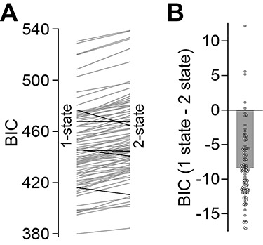
Validation of the single state-space model. A. We calculated the Bayesian Information Criterion (BIC) for single- and two-state model fits to individual subject behavior. The endpoint of each line shows the average BIC for the A and B periods (left, single-state model; right, two-state model). Each line depicts the result for a single subject. Black lines indicate subjects for which the two-state model was superior to the single-state model. B. We calculated the difference in BIC for the single-state and two-state models. Negative values indicate higher evidence for the single-state model. The bar depicts mean BIC, and error bars indicate ±1 standard error of the mean. Data for each subject is superimposed in gray.

The state-space model assumes that learning is governed by two processes: a process that learns from error and a process that retains a fraction of that memory from one trial to the next. The model closely tracked the observed behavior (Fig. 4A).

Figure 4.

State-space model fit. A. We fit individual behavior using a single-state model that estimated cycle-by-cycle forgetting, error-based learning, and initial bias. Each plot depicts the median pointing angle for each experimental group (gray lines) as well as the median pointing angle predicted from simulating the state-space model without noise (black lines) using the maximum likelihood model parameter sets identified for each subject. Behavior and state-space predictions are provided for the control group in the top left plot. The shaded error region indicates ±1 standard error of the median. B. Initial state of the learner at the start of the B period. C. Error sensitivity during the B period. D. Retention factor during the B period. In panels E–G, we repeated our primary analysis, excluding the initial cycles of large errors from the model fit. To this aim, based on our exponential model, we selected the cycle during which the pointing angle was nearest zero. E. New initial pointing angle for this analysis (black) and the true initial pointing angles at the start of B (gray). F. Error sensitivity of a state-space model after removing the initial period of large errors. G. Error sensitivity of the state-space model fit after removing the initial period of large errors (black) and fit to the entire B period (gray). Each bar represents the mean (B and E) or median (C, D, F, and G) parameter value for each group. Error bars indicate ±1 standard error of the mean or median. Data for each subject is superimposed in gray. Asterisks indicate a level of significance of P < 0.05 (^*), P < 0.01 (^**), or P < 0.001 (^***).

To quantify the model’s goodness of fit, we computed the fraction of each subject’s behavioral variance accounted for by our model fit (R₂). To measure this coefficient of determination, we computed the expected value of the behavior predicted by our stochastic model (eqs. 2 and 3) and compared this prediction with each individual subject’s data. We found that for single subjects, our model accounted for approximately 81.4 ± 8.4% (mean ± 1 std. dev.) of the variance in subject behavior. We repeated this analysis at the group level, where noise in the process of learning (eq. 2) and production of a movement (eq. 3) is smoothed over subjects. For each group, we computed the median behavior, the median behavior predicted by our model (Fig. 4A), and then the coefficient of determination for these two time courses. At the group level, the model accounted for 96.0–98.2% of the variance in median subject behavior.

Using the model parameters, we measured the impact of prior learning on (1) biases in performance due to the memory of A, (2) the rate of memory decay in B, and (3) the capacity to learn from error in B. These three processes are represented separately by three specific model parameters: (1) initial state of the learner in B, (2) retention factor, and (3) error sensitivity.

Unsurprisingly, the initial state of the learner in B (Fig. 4B) closely followed our empirical estimate of the initial level of performance in B (Fig. 2A). As the interval between A and B increased, the initial state of the learner in B, that is, the amount of the A memory retained over time, decreased (one-way ANOVA, F_(88,4) = 52.16, P < 0.001; Dunnett’s test, control different from all experimental groups with P < 0.001; Tukey’s test, 5 min different than 24 h with P = 0.023, all other comparisons are nonsignificant). However, despite this temporal decay, all experimental groups retained at least 50% of the memory of A (one-sample t-test with Bonferroni correction, all experimental groups P < 0.001), while the control group was not different from zero (P = 0.11). Therefore, impairment of performance in B was in part caused by a lingering memory of A that was present even at 24 h.

To what extent was the impairment in B driven by changes in the rate of error-based learning and the strength of memory retention? Similar to our empirical analysis, we first confirmed that the experimental groups did not differ in performance during the A period. That is, there was no difference in error sensitivity (Kruskal–Wallis, X²(65) = 1.16, P = 0.763) or retention factor (Kruskal–Wallis, X²(66) = 0.53, P = 0.912) across the experimental groups during adaptation to A. Yet, we found that error sensitivity was affected by prior learning (Fig. 4C; Kruskal–Wallis, X²(83) = 14.47, P = 0.006). Post hoc tests against the control group unveiled a significant reduction in error sensitivity at 5 min and 1 h but not at longer time intervals (Dunn’s test with Bonferroni correction, 5 min different from control with P = 0.008, 1 h different from control with P = 0.004, 6 and 24 h not different from control with P > 0.132). In contrast, we found no difference in the retention factor during learning in B for any of the experimental groups, including the control group (Fig. 4D; Kruskal–Wallis, X²(79) = 5.66, P = 0.226).

In summary, our state-space model pointed to a similar conclusion drawn from our empirical findings. Prior exposure to A resulted in a bias in the initial state of B that persisted through 24 h. However, despite this lingering initial bias, prior exposure produced a short-lived impairment in error sensitivity: error sensitivity in B resembled control values when the time between A and B was 6 h or more. Therefore, differences in performance in B for any time scale greater than 6 h were likely related to a prior memory of A and not to a deficit in learning.

Error Sensitivity Is Independent of Initial Error Size

We and others have shown that sensitivity to error declines as a function of error size (Kim et al. 2018; Marko et al. 2012; Wei and Körding 2009). This raises the concern that the differences in error sensitivity reported in Fig. 4C may be driven by the differences in the magnitude of the initial error experienced at the start of perturbation B. To address this possibility, we reanalyzed behavior in B, this time controlling for initial error size. To this aim, we fit an exponential function (eq. 1) and identified the cycle in which each participant exhibited a pointing angle near zero and refit our state-space model to the behavior after this point. In this way, model parameters could no longer be impacted by differences in initial error size across groups (Fig. 4E). We found that the pattern of error sensitivity described when fitting the whole behavior (Fig. 4C; Kruskal–Wallis, X²(83) = 14.47, P = 0.006; Dunn’s test 5 min vs. control, P = 0.008; Dunn’s test 1 hour vs. control, P = 0.004) persisted even when the initial error was near zero (Fig. 4F; Kruskal–Wallis, X²(81) = 11.25, P = 0.024; Dunn’s test 5 min vs. control, P = 0.041; Dunn’s test 1 hour vs. control, P = 0.007). Furthermore, no significant differences were found when the two analyses were compared (Fig. 4G; Wilcoxon signed rank test for each experimental group with Bonferroni correction, P > 0.177 for all groups).

In conclusion, these results indicate that the impact of prior learning on error sensitivity cannot be explained by the initial level of error experienced in B. Rather, the effect appears to be related to a deficit in the ability to learn.

Alternate Hypotheses: A Two-State Model Account of Anterograde Interference

The decrease in error sensitivity observed here is at odds with a prior account of anterograde interference in force field adaptation (Sing and Smith 2010), in which an impairment of learning arises from differing initial biases in the underlying adaptive states of a two-state system, rather than a change in sensitivity to error. Briefly, in the two-state framework, learning in B is hindered when the slower state of learning is biased toward earlier adaptation. We tested this idea in a supplementary analysis using a two-state model and found that it fails to account for our empirical data (Supplementary file 1). Therefore, the fact that the slow state is heavily biased toward A at the start of B cannot explain the deficit we observed in the speed of learning in B. In fact, fitting a two-state model in which parameters are free to vary from A to B (Supplementary file 2) yields a similar pattern of impairment in error sensitivity of the slow module to the one obtained with a single-state model, with no impact of anterograde interference on the fast module. This analysis suggests that the recovery of behavior we observe over time was not caused by the interaction of the fast and slow states (i.e., the initial bias) but rather by the restoration of error sensitivity of the slow process. Altogether, our findings indicate that anterograde interference in visuomotor adaptation is caused by a genuine impairment in error sensitivity both for one-state and two-state models of learning.

Discussion

How do motor memories influence one another? In this work, we studied the expression of anterograde interference in visuomotor adaptation by varying the time elapsed between learning opposing perturbations. We examined the impact of prior learning on the initial level of performance as well as the rate of learning over the time course of 5 min through 24 h. We found that these two parameters behaved very differently as a function of time. On one hand, adaptation in A biased the initial level of performance in B. Although the magnitude of this effect decreased with time, it remained strong at 24 h. On the other hand, prior adaptation impaired the ability to learn from error, resulting in reduced error sensitivity when perturbations were separated by 5 min and 1 h. Unlike the bias caused by prior learning, error sensitivity recovered with the passage of time. To the best of our knowledge, these findings demonstrate for the first time that anterograde interference, a fundamental concept in memory research, is caused by a reduction in error sensitivity that recovers over time.

Anterograde Interference Differs from a Lingering Memory of a Prior

There has been no general agreement in the sensorimotor literature regarding how to define and, therefore, quantify anterograde interference. With the exception of Sing and Smith (2010), who measured the relative change in learning rate, most previous studies estimated anterograde interference based on the initial level of performance, by averaging across the first trials/cycles/blocks (Brashers-Krug et al. 1996; Krakauer et al. 2005; Lee and Schweighofer 2009; Shadmehr and Brashers-Krug 1997; Tong and Flanagan 2003). For example, Tong and Flanagan (2003) reported interference at 5 min based on the average of the second and third cycles. Likewise, Miall et al. (2004) reported interference at 15 min based on the initial state obtained from fitting a power function, while noting that the rate of learning was not affected. Yet, it is likely that the initial level of performance, when averaged across trials, reflects not only the capacity for learning in B but also the bias of a lingering memory of A. Evidence supporting this possibility comes from force field studies showing that the preferred direction of the biceps and triceps during exposure to a second opposing force field is appropriate to solve the first force field (e.g., Thoroughman and Shadmehr 1999). Therefore, assessing anterograde interference based on the initial level of performance may overestimate its magnitude.

Here, we compared the bias imposed by the memory of A with the deficit observed in the rate of learning. We reasoned that if, as suggested by previous work, the initial level of performance reflects the level of anterograde interference, then the two measures should behave similarly as a function of time. In contrast, we found that initial performance was profoundly hindered throughout the 24 h of testing whereas the ability to learn resembled control levels starting at 6 h. Furthermore, the fact that the pattern of error sensitivity persisted when controlling for initial error size suggests that anterograde interference is caused by a genuine downregulation of error sensitivity.

Anterograde Interference and Memory Stabilization

Our work sheds light on a long-standing debate regarding the failure of retrograde protocols at unveiling the time course of memory consolidation. Over the past two decades, several laboratories have attempted to uncover the time course of memory stabilization using behavioral protocols based on retrograde interference (e.g., Brashers-Krug et al. 1996; Caithness et al. 2004; Krakauer et al. 2005). In these studies, subjects usually adapt to opposing perturbations A (A₁) and B separated by a time interval that varies between minutes to 24 h. Next, they wait for a further period of time (usually 24 h) and are again exposed to A (A₂) to assess the integrity of the motor memory. Consolidation of the memory of A should be reflected as the presence of savings (a faster rate of learning) in A₂. Although this approach has proved successful in declarative (Lechner et al. 1999; Tulving 1969) and some kinds of motor skill learning tasks (Korman et al. 2007; Walker et al. 2003), it has led to inconclusive results in sensorimotor adaptation. In fact, with the exception of three force field studies reporting release from interference at around 6 h (Brashers-Krug et al. 1996; Shadmehr and Brashers-Krug 1997) or later (Overduin et al. 2006), other experiments have shown complete lack of savings even if 24 h is interposed between A₁ and B (Bock et al. 2001; Caithness et al. 2004; Goedert and Willingham 2002; Krakauer et al. 2005). These inconsistencies have also been reported for perceptual and motor sequence learning, prism adaptation (Aberg and Herzog 2010; Goedert and Willingham 2002), and declarative tasks including the paired associate task (Houston 1967; Howe 1969; McGeoch 1933; Wixted 2004). Miall et al. (2004) have claimed that naïve performance at recall (A₂) reported in retrograde protocols (Caithness et al. 2004; Goedert and Willingham 2002; Krakauer et al. 2005) reflects a mixture of anterograde interference from B and the integrity of the memory of A, and not catastrophic retrograde interference. It is important to note, however, that these authors measured anterograde interference based on the initial level of performance. In light of our findings, the interpretation of these studies may need to be revisited. Our data indicates that, because release from interference starts at around 6 h, anterograde interference is not likely to cause naïve performance in A₂. Tracking the time course of recovery in learning rate reported here provides a new path forward for understanding the process of memory stabilization.

The temporal dissociation we observed between the initial level of performance and the rate of learning likely reflects the contribution of two distinct processes: (1) the persistence of a prior memory and (2) competition for neural resources that support learning. The formation of memory involves learning-dependent synaptic plasticity as part of a process known as long-term potentiation and depression (LTP and LTD). Given that biological substrates underlying synaptic plasticity are limited by nature, cellular modifications induced by learning temporarily constrain the capacity for further LTP induction. This phenomenon is known as occlusion and reflects competition for neural resources that support plasticity (Ling et al. 2002). Using this approach, it has been reported that motor skill learning in rats and humans is associated with LTP (Cantarero et al. 2013; Rioult-Pedotti et al. 1998; Rioult-Pedotti et al. 2000). Cantarero and collaborators showed that in fact, in humans, occlusion fades around 6 h after motor skill learning. In this light, we may speculate that adaptation in A may have partially occluded the capacity for further synaptic plasticity, thereby hindering adaptation in B. The timing of recovery from interference we describe here (starting around 6 h) coincides with the peak in functional connectivity of a visuomotor adaptation network that includes the primary motor cortex (M1), the posterior parietal cortex (PPC), and the cerebellum (Della-Maggiore et al. 2017). The timing of recovery is also in general agreement with recent results showing that in the minutes after conclusion of reach adaptation, the retention of the acquired memory depends on the somatosensory cortex, but this dependence is no longer present at 24 h (Kumar et al. 2019). These regions have been linked to memory formation in visuomotor rotation (Della-Maggiore et al. 2004; Hadipour-Niktarash et al. 2007; Landi et al. 2011; Richardson et al. 2006). Whether this timing reflects the process of motor memory consolidation is now a hypothesis amenable for testing.

Anterograde Interference Results From an Impairment in Error Sensitivity that Recovers with Time

Using a state-space model allowed us to identify which aspect of learning was affected by anterograde interference, that is, a deficit in the ability to learn from error or in the ability to retain information cycle-by-cycle. Here we found that anterograde interference could be attributed to a change in error sensitivity. It is well established that humans have the ability to change their error sensitivity depending on the errors they have experienced in the past (Gonzalez Castro et al. 2014). Current models of error sensitivity (Herzfeld et al. 2014) posit that sensitivity to a specific error increases gradually in an environment where that error is likely to occur again on the next trial and decreases gradually if the error is unlikely to occur again. In this way, sensitivity to an error is specific to one’s prior history of error. However, the decrease in error sensitivity we report here is of a different nature. Here, error sensitivity in B is reduced even though errors in B were never experienced during the A perturbation. This points to a different mechanism for error sensitivity modification, one in which learning of a perturbation actively suppresses learning of a different perturbation, potentially through a competition for neural resources that subsides at longer time intervals.

Substantial evidence indicates that visuomotor adaptation results from the interplay between explicit learning (driven by target error) and implicit learning (driven by prediction error) (Haith et al. 2015; Morehead et al. 2015; Taylor et al. 2014; Tseng et al. 2007). Could the changes we observed in error sensitivity be caused by differential contributions of implicit and explicit components of learning? This possibility is unlikely for two reasons. The reaction time (a marker for explicit learning) of experimental and control groups was similar in B (Supplementary file 3), suggesting that the relative implicit/explicit contribution to adaptation did not change with the amount of time separating A and B. In addition, the pattern of error sensitivity persisted even after the critical early cycles, generally associated with the use of explicit strategies, were excluded (compare Fig. 4C,F). Together, these results undermine the possibility that differences in the relative implicit/explicit contributions could account for our results.

In conclusion, we have examined the strength and duration of anterograde interference in visuomotor adaptation by tracking its impact on behavior during learning of opposing perturbations separated from 5 min through 24h. We found that prior learning dramatically hindered the initial state at all time intervals. This was likely due to a bias imposed by a lingering memory associated with adapting to the initial perturbation. Prior learning also impaired the ability to learn from errors for at least 1 h, but a release from interference was detected starting as early as 6 h post training. This finding is consistent with a process of memory stabilization for this type of learning. Our work suggests that the poor performance observed when opposing rotations are learned consecutively is driven by two distinct phenomena operating on different time scales (days vs. hours): a long-lasting influence of a memory that acts as a prior which negatively influences the initial level of performance and a shorter-lasting impairment of learning.

Funding

Argentinian Ministry of Defense (PIDDEF); Argentinian Agency for the promotion of Science and Technology (FONCyT, ANPCyT); University of Buenos Aires (UBACyT); National Institutes of Health (R01-NS078311, R01-NS095706 to R.S.). National Institutes of Health (NS-095706 to S.A.).

Notes

Conflict of Interest: None declared.

References

- Aberg KC, Herzog MH. 2010. Does perceptual learning suffer from retrograde interference? PLoS One. 5:e14161. [DOI] [PMC free article] [PubMed] [Google Scholar]
- Albert ST, Shadmehr R. 2018. Estimating properties of the fast and slow adaptive processes during sensorimotor adaptation. J Neurophysiol. 119:1367–1393. [DOI] [PMC free article] [PubMed] [Google Scholar]
- Bock O, Schneider S, Bloomberg J. 2001. Conditions for interference versus facilitation during sequential sensorimotor adaptation. Exp Brain Res. 138:359–365. [DOI] [PubMed] [Google Scholar]
- Brainard DH. 1997. The Psychophysics Toolbox. Spat Vis. 10:433–436. [PubMed] [Google Scholar]
- Brashers-Krug T, Shadmehr R, Bizzi E. 1996. Consolidation in human motor memory. Nature. 382:252–255. [DOI] [PubMed] [Google Scholar]
- Braun DA, Aertsen A, Wolpert DM, Mehring C. 2009. Motor task variation induces structural learning. Curr Biol. 19:352–357. [DOI] [PMC free article] [PubMed] [Google Scholar]
- Caithness G, Osu R, Bays P, Chase H, Klassen J, Kawato M, Wolpert D, Flanagan J. 2004. Failure to consolidate the consolidation theory of learning for sensorimotor adaptation tasks. J Neurosci. 24:8662–8671. [DOI] [PMC free article] [PubMed] [Google Scholar]
- Cantarero G, Tang B, O’Malley R, Salas R, Celnik P. 2013. Motor learning interference is proportional to occlusion of LTP-like plasticity. J Neurosci. 33:4634–4641. [DOI] [PMC free article] [PubMed] [Google Scholar]
- Cheng S, Sabes PN. 2006. Modeling sensorimotor learning with linear dynamical systems. Neural Comput. 18:760–793. [DOI] [PMC free article] [PubMed] [Google Scholar]
- Della-Maggiore V, Malfait N, Ostry DJ, Paus T. 2004. Stimulation of the posterior parietal cortex interferes with arm trajectory adjustments during the learning of new dynamics. J Neurosci. 24:9971–9976. [DOI] [PMC free article] [PubMed] [Google Scholar]
- Della-Maggiore V, Villalta JI, Kovacevic N, McIntosh AR. 2017. Functional evidence for memory stabilization in sensorimotor adaptation: a 24-h resting-state fMRI study. Cereb Cortex. 27:1748–1757. [DOI] [PubMed] [Google Scholar]
- Donchin O, Francis JT, Shadmehr R. 2003. Quantifying generalization from trial-by-trial behavior of adaptive systems that learn with basis functions: theory and experiments in human motor control. J Neurosci. 23:9032–9045. [DOI] [PMC free article] [PubMed] [Google Scholar]
- Ethier V, Zee DS, Shadmehr R. 2008. Spontaneous recovery of motor memory during saccade adaptation. J Neurophysiol. 99:2577–2583. [DOI] [PMC free article] [PubMed] [Google Scholar]
- Goedert KM, Willingham DB. 2002. Patterns of interference in sequence learning and prism adaptation inconsistent with the consolidation hypothesis. Learn Mem. 9:279–292. [DOI] [PMC free article] [PubMed] [Google Scholar]
- Gonzalez Castro LN, Hadjiosif AM, Hemphill MA, Smith MA. 2014. Environmental consistency determines the rate of motor adaptation. Curr Biol. 24:1050–1061. [DOI] [PMC free article] [PubMed] [Google Scholar]
- Hadipour-Niktarash A, Lee CK, Desmond JE, Shadmehr R. 2007. Impairment of retention but not acquisition of a visuomotor skill through time-dependent disruption of primary motor cortex. J Neurosci. 27:13413–13419. [DOI] [PMC free article] [PubMed] [Google Scholar]
- Haith AM, Huberdeau DM, Krakauer JW. 2015. The influence of movement preparation time on the expression of visuomotor learning and savings. J Neurosci. 35:5109–5117. [DOI] [PMC free article] [PubMed] [Google Scholar]
- Herzfeld DJ, Vaswani PA, Marko MK, Shadmehr R. 2014. A memory of errors in sensorimotor learning. Science (80- ). 345:1349–1353. [DOI] [PMC free article] [PubMed] [Google Scholar]
- Houston JP. 1967. Stimulus selection as influenced by degrees of learning, attention, prior associations, and experience with the stimulus components. J Exp Psychol. [DOI] [PubMed] [Google Scholar]
- Howe TS. 1969. Effects of delayed interference on list 1 recall. J Exp Psychol. 80:120–124. [Google Scholar]
- Kim HE, Morehead JR, Parvin DE, Moazzezi R, Ivry RB. 2018. Invariant errors reveal limitations in motor correction rather than constraints on error sensitivity. Commun Biol. 1:19. [DOI] [PMC free article] [PubMed] [Google Scholar]
- Korman M, Doyon J, Doljansky J, Carrier J, Dagan Y, Karni A. 2007. Daytime sleep condenses the time course of motor memory consolidation. Nat Neurosci. 10:1206–1213. [DOI] [PubMed] [Google Scholar]
- Krakauer JW. 2009. Motor Learning and Consolidation: The Case of Visuomotor Rotation. Adv Exp Med Biol. 629:405–21. [DOI] [PMC free article] [PubMed] [Google Scholar]
- Krakauer JW, Ghez C, Ghilardi MF. 2005. Adaptation to visuomotor transformations: consolidation, interference and forgetting. J Neurosci. 25:473–478. [DOI] [PMC free article] [PubMed] [Google Scholar]
- Kumar N, Manning TF, Ostry DJ. 2019. Somatosensory cortex participates in the consolidation of human motor memory. PLoS Biol. 17:e3000469. [DOI] [PMC free article] [PubMed] [Google Scholar]
- Landi SM, Baguear F, Della-Maggiore V. 2011. One week of motor adaptation induces structural changes in primary motor cortex that predict long-term memory one year later. J Neurosci. 31:11808–11813. [DOI] [PMC free article] [PubMed] [Google Scholar]
- Lechner HA, Squire LR, Byrne JH. 1999. 100 years of consolidation—remembering Müller and Pilzecker. Learn Mem. 6:77–87. [PubMed] [Google Scholar]
- Lee J-Y, Schweighofer N. 2009. Dual adaptation supports a parallel architecture of motor memory. J Neurosci. 29:10396–10404. [DOI] [PMC free article] [PubMed] [Google Scholar]
- Leow LA1, Hammond G, de Rugy A.. 2014. Anodal motor cortex stimulation paired with movement repetition increases anterograde interference but not savings. Eur J Neurosci. 40:3243–52. [DOI] [PubMed] [Google Scholar]
- Ling DSF, Benardo LS, Serrano PA, Blace N, Kelly MT, Crary JF, Sacktor TC. 2002. Protein kinase Mζ is necessary and sufficient for LTP maintenance. Nat Neurosci. 5:295–296. [DOI] [PubMed] [Google Scholar]
- Marko MK, Haith AM, Harran MD, Shadmehr R. 2012. Sensitivity to prediction error in reach adaptation. J Neurophysiol. 108:1752–1763. [DOI] [PMC free article] [PubMed] [Google Scholar]
- McGeoch JA. 1933. The formal criteria of a systematic psychology. Psychol Rev. 40:1–12. [Google Scholar]
- Miall RC, Jenkinson N, Kulkarni K. 2004. Adaptation to rotated visual feedback: a re-examination of motor interference. Exp Brain Res. 154:201–210. [DOI] [PubMed] [Google Scholar]
- Morehead JR, Qasim SE, Crossley MJ, Ivry R. 2015. Savings upon re-aiming in visuomotor adaptation. J Neurosci. 35:14386–14396. [DOI] [PMC free article] [PubMed] [Google Scholar]
- Oldfield RC. 1971. The assessment and analysis of handedness: the Edinburgh inventory. Neuropsychologia. 9:97–113. [DOI] [PubMed] [Google Scholar]
- Overduin SA, Richardson AG, Lane CE, Bizzi E, Press DZ. 2006. Intermittent practice facilitates stable motor memories. J Neurosci. 26:11888–11892. [DOI] [PMC free article] [PubMed] [Google Scholar]
- Pekny SE, Criscimagna-Hemminger SE, Shadmehr R. 2011. Protection and expression of human motor memories. J Neurosci. 31:13829–13839. [DOI] [PMC free article] [PubMed] [Google Scholar]
- Richardson AG, Overduin SA, Valero-Cabre A, Padoa-Schioppa C, Pascual-Leone A, Bizzi E, Press DZ. 2006. Disruption of primary motor cortex before learning impairs memory of movement dynamics. J Neurosci. 26:12466–12470. [DOI] [PMC free article] [PubMed] [Google Scholar]
- Rioult-Pedotti M-S, Friedman D, Hess G, Donoghue JP. 1998. Strengthening of horizontal cortical connections following skill learning. Nat Neurosci. 1:230–234. [DOI] [PubMed] [Google Scholar]
- Rioult-Pedotti MS, Friedman D, Donoghue JP. 2000. Learning-induced LTP in neocortex. Science. 290:533–536. [DOI] [PubMed] [Google Scholar]
- Shadmehr R, Brashers-Krug T. 1997. Functional stages in the formation of human long-term motor memory. J Neurosci. 17:409–419. [DOI] [PMC free article] [PubMed] [Google Scholar]
- Sing GC, Smith MA. 2010. Reduction in learning rates associated with anterograde interference results from interactions between different timescales in motor adaptation. PLoS Comput Biol. 6:e1000893. [DOI] [PMC free article] [PubMed] [Google Scholar]
- Sing GC, Joiner WM, Nanayakkara T, Brayanov JB, Smith MA. 2009. Primitives for motor adaptation reflect correlated neural tuning to position and velocity. Neuron. 64:575–589. [DOI] [PubMed] [Google Scholar]
- Smith MA, Ghazizadeh A, Shadmehr R. 2006. Interacting adaptive processes with different timescales underlie short-term motor learning. PLoS Biol. 4:e179. [DOI] [PMC free article] [PubMed] [Google Scholar]
- Taylor JA, Krakauer JW, Ivry RB. 2014. Explicit and implicit contributions to learning in a sensorimotor adaptation task. J Neurosci. 34:3023–3032. [DOI] [PMC free article] [PubMed] [Google Scholar]
- Thoroughman KA, Shadmehr R. 1999. Electromyographic correlates of learning an internal model of reaching movements. J Neurosci. 19:8573–8588. [DOI] [PMC free article] [PubMed] [Google Scholar]
- Thoroughman KA, Shadmehr R. 2000. Learning of action through adaptive combination of motor primitives. Nature. 407:742–747. [DOI] [PMC free article] [PubMed] [Google Scholar]
- Tong C, Flanagan JR. 2003. Task-specific internal models for kinematic transformations. J Neurophysiol. 90:578–585. [DOI] [PubMed] [Google Scholar]
- Tseng Y, Diedrichsen J, Krakauer JW, Shadmehr R, Bastian AJ. 2007. Sensory prediction errors drive cerebellum-dependent adaptation of reaching. J Neurophysiol. 98:54–62. [DOI] [PubMed] [Google Scholar]
- Tulving E. 1969. Retrograde amnesia in free recall. Science (80-). 164:88–90. [DOI] [PubMed] [Google Scholar]
- Vaswani PA, Shmuelof L, Haith AM, Delnicki RJ, Huang VS, Mazzoni P, Shadmehr R, Krakauer JW. 2015. Persistent residual errors in motor adaptation tasks: reversion to baseline and exploratory escape. J Neurosci. 35:6969–6977. [DOI] [PMC free article] [PubMed] [Google Scholar]
- Walker MP, Brakefield T, Allan Hobson J, Stickgold R. 2003. Dissociable stages of human memory consolidation and reconsolidation. Nature. 425:616–620. [DOI] [PubMed] [Google Scholar]
- Wei K, Körding K. 2009. Relevance of error: what drives motor adaptation? J Neurophysiol. 101:655–664. [DOI] [PMC free article] [PubMed] [Google Scholar]
- Wigmore V, Tong C, Flanagan JR. 2002. Visuomotor rotations of varying size and direction compete for a single internal model in a motor working memory. J Exp Psychol Hum Percept Perform. 28:447–457. [DOI] [PubMed] [Google Scholar]
- Wixted JT. 2004. The psychology and neuroscience of forgetting. Annu Rev Psychol. 55:235–269. [DOI] [PubMed] [Google Scholar]
- Zarahn E, Weston GD, Liang J, Mazzoni P, Krakauer JW. 2008. Explaining savings for visuomotor adaptation: linear time-invariant state-space models are not sufficient. J Neurophysiol. 100:2537–2548. [DOI] [PMC free article] [PubMed] [Google Scholar]
Associated Data
This section collects any data citations, data availability statements, or supplementary materials included in this article.