Experimental investigation of far‐field human cough airflows from healthy and influenza‐infected subjects

Abstract

Seasonal influenza epidemics have been responsible for causing increased economic expenditures and many deaths worldwide. Evidence exists to support the claim that the virus can be spread through the air, but the relative significance of airborne transmission has not been well defined. Particle image velocimetry (PIV) and hot‐wire anemometry (HWA) measurements were conducted at 1 m away from the mouth of human subjects to develop a model for cough flow behavior at greater distances from the mouth than were studied previously. Biological aerosol sampling was conducted to assess the risk of exposure to airborne viruses. Throughout the investigation, 77 experiments were conducted from 58 different subjects. From these subjects, 21 presented with influenza‐like illness. Of these, 12 subjects had laboratory‐confirmed respiratory infections. A model was developed for the cough centerline velocity magnitude time history. The experimental results were also used to validate computational fluid dynamics (CFD) models. The peak velocity observed at the cough jet center, averaged across all trials, was 1.2 m/s, and an average jet spread angle of θ = 24° was measured, similar to that of a steady free jet. No differences were observed in the velocity or turbulence characteristics between coughs from sick, convalescent, or healthy participants.

Practical Implications.

• The present work can be useful when quantifying air movement from coughs in healthcare settings.

• The results of the study can be used to identify safe separation distances and to develop preventative measures for the mitigation of person-to-person virus transmission.

1. INTRODUCTION

Communicable respiratory diseases have demonstrated the potential to cause global pandemics, which has resulted in increased economic expenditure, and many deaths worldwide. ¹ , ² The significance of the airborne route of virus transmission has been a topic of recent interest in the healthcare community. An outbreak of SARS‐CoV‐2 (COVID‐19) in December 2019 was the third major epidemic in the last 20 years caused by an animal coronavirus that had been transmitted to humans. ³ At the time of writing, there have been 45 171 confirmed infections and 1115 deaths worldwide attributed to COVID‐19. ⁴

Respiratory activities, such as coughing, sneezing, breathing, and talking, generate and disperse pathogen‐bearing droplets and aerosols. ⁵ The distance that these particles travel depends on both the size of the particle and the velocity at which it is expired. ⁶ Although large droplets play a significant role in virus transmission, they are expected to fall more quickly and are less likely to be inhaled. Several reviews support the claim that droplet nuclei smaller than 5 μm behave much like a gas and are capable of remaining suspended within the air for long periods of time, and may contribute to airborne virus transmission. ⁷ , ⁸

Several studies have tried to determine the size distribution of aerosolized particles produced by coughing, but the distributions varied between experiments. ⁹ , ¹⁰ , ¹¹ , ¹² , ¹³ It has been indicated that 99% of all expired particles are smaller than 10 μm and they can be easily inhaled by a susceptible host. By taking measurements of particles in their equilibrium states (after all volatile water content has evaporated), a multi‐modal distribution of particle sizes with peaks at 1 and 100 μm has been observed. ¹¹ , ¹² Biological sampling has confirmed the presence of viable pathogens within these aerosols. ¹⁴ , ¹⁵ , ¹⁶ Experimental investigations concerning subjects who have been naturally infected with influenza have shown that 65% of influenza RNA was found in particles smaller than 4 μm, although the presence of influenza RNA does not necessarily indicate the presence of viable viruses. ¹⁵ However, such investigations were conducted at or near the mouth of subjects.

The velocity at which infectious particles are introduced into the environment influences the potential for transmission. Several investigations have been conducted to examine the flow behavior of coughs at or near the mouth of human subjects, ¹⁷ , ¹⁸ , ¹⁹ , ²⁰ , ²¹ , ²² , ²³ , ²⁴ , ²⁵ but only one investigation has examined cough flow behavior beyond this region. ²⁶ While determining the cough flow behavior close to the mouth can be useful for determining boundary conditions for numerical or physical simulations, the flow behavior in the far field is more important when assessing the potential for virus transmission, since such separation distances are more common for most human interactions. Volumetric flow rates, volumes, and peak velocity times of coughs have been determined using spirometry techniques, ¹⁷ , ²¹ whereas shadowgraph techniques, ²² video imaging, ²⁴ , ²⁵ and particle image velocimetry (PIV) ¹⁸ , ¹⁹ , ²⁰ , ²³ , ²⁶ have been used to visualize the flow field. The experimental results vary significantly between experiments and between subjects, and no well‐defined model exists for near‐field or far‐field cough behavior. Furthermore, the separation distance that distinguishes between the near field and far field of cough flow behavior has not been defined. All previous investigations of the flow field have been conducted with healthy subjects and so there is no evidence indicating that coughs from subjects who have been naturally infected with respiratory viruses behave like those from healthy subjects. Statistical issues also become evident, due to the small number of subjects recruited for the experiments.

Very little is known about the production and dispersion of viral bioaerosols, even though such information is critical in healthcare settings during viral outbreaks. Viable influenza particles have been recovered through air sampling at hospitals, at health centers, and on airplanes, ²⁷ , ²⁸ , ²⁹ and several factors have been shown to influence airborne transmission of the influenza virus. Guinea pig models have demonstrated that low relative humidity (RH) and low temperatures enhanced the transmission of the influenza virus, whereas high RH and high temperatures interrupted transmission. ³⁰ , ³¹ , ³³ Despite this, there is a widespread adoption of the “3 ft/1 m” and “6 ft/2 m” rules, ³⁴ , ³⁵ which have considered such separation distances from patients infected with respiratory viruses to be safe, without any evidence to support the claim.

The objective of the present investigation was to test the “3 ft/1 m rule,” by conducting velocity measurements and bioaerosol sampling at x = 1.0 m from the mouth of human subjects. Based on an average mouth opening diameter of D = 0.02 m, ²¹ this region is calculated to be approximately x = 50D. Experiments were conducted to map the flow field of human coughs at greater distances than those studied previously and to develop a model for transient cough jet behavior. Subjects who have been naturally infected with influenza participated in experiments while they were sick and again when they had recovered. A cohort of healthy volunteers was recruited as a reference to assess any difference in the aerodynamic behavior of the coughs from the two groups. The velocity measurements were also used to validate computational fluid dynamics (CFD) models based on unsteady Reynolds‐averaged Navier‐Stokes (URANS) and large eddy simulation (LES) methods developed by Bi. ³⁶ While it has been demonstrated that viral aerosols are typically expired from breathing, ³⁷ the present investigation focuses solely on the fluid mechanics of coughing, since there is a potential for the transportation of aerosols and droplets further from the source.

2. METHODOLOGY

2.1. Experimental facility and procedure

The experimental chamber ²⁴ consisted of a 1.81 m × 1.81 m × 1.78 m enclosure, with all interior surfaces painted black, except for a glass window allowing optical access and a glass panel in the center of the chamber (Figure 1). The dimensions of the chamber were selected so that the cough airflow was not noticeably influenced by the chamber walls. A pear‐shaped opening, with a padded head rest and chin rest, fixed the participant's head in place, but allowed the participant to cough into the chamber with their nose and mouth unobstructed. Subjects were asked to cough 3 times each in separate particle image velocimetry (PIV) and hot‐wire anemometry (HWA) experiments with aerosol sampling. Participants waited for approximately 2 minutes between coughs to minimize the residual air motion within the chamber.

Figure 1.

Schematic diagram of experimental facility

2.2. Particle image velocimetry (PIV)

PIV has commonly been used as a non‐intrusive technique to measure airflow fields due to its accuracy and spatial resolution. For PIV experiments, the chamber was seeded with aerosolized titanium dioxide (TiO₂) particles (ranging between 0.15 and 0.47 µm with 69% of particles between 0.34 and 0.43 µm) that were dried in a vacuum oven. The particles were stored in a drum, which was placed on top of a loudspeaker that vibrated to aerosolize the powder. The seeding particles were carried into the chamber from the drum by a 30 kPa airline. Particles were illuminated by a 120 mJ per pulse, 532‐nm Nd:YAG laser, which was directed through an angled mirror and a cylindrical/spherical lens assembly to create a laser sheet (~1 mm thickness). Each pulse has a duration of 3‐5 ns, and synchronized image pairs were recorded by a CCD camera at a frequency of 15 Hz (2017‐18 experiments) and 16.7 Hz (2013‐14 experiments). ²⁶ An image separation time of Δt = 100 µs was used, while laser pulse delay and PIV exposure times of 400 and 405 µs were selected, respectively. Overall, a velocity uncertainty of 0.04 m/s was associated with the sum of pixel errors. Based on the approximate average peak measured velocity of V = 1.1 m/s, an uncertainty of 3.6% was observed.

In the experiments conducted in 2013‐14, much of the cough flow missed the small field of view in some trials, and many coughs missed completely. To contain the entire width of the cough within the imaged window and due to a necessary change in the camera used, a new field of view was selected for the experiments conducted in 2017‐18 (Figure 2). Both windows were centered at x = 1 m downstream from the participant, and they were translated downward to compensate for the typically downward initial cough trajectory. ²¹ A recursive Nyquist cross‐correlation algorithm was used, in TSI Insight 4G software, to process images into velocity vector arrays. A final spot dimension of 32 × 32 pixels was used for the 2013‐14 images, whereas it was increased to 64 × 64 pixels to compensate for the decrease in spatial resolution from 10.0 to 6.87 pixels/mm. Since the camera is farther from the laser sheet, increasing the field of view, a larger final spot dimension is necessary to ensure the proportion of validated vectors is over 85%. Eighty image pairs are recorded for each cough, allowing enough time for the cough to pass the field of view completely. The time at which the cough first reaches the measurement location was set to be t = 0.0 seconds.

Figure 2.

PIV field of view on cough chamber center plane

Time histories for the 2D instantaneous velocity magnitude, V, were computed according to Equation 1.

$$V=\sqrt{u^2+v^2}$$ (1)

where u is the streamwise velocity component in the x‐direction, and v is the vertical component in the y‐direction.

The time histories were extracted at the cough jet center, as well as at the chamber centerline and the HWA location, x = 1 m away from the subject. After examining the velocity contours and vector arrays, the cough jet center was defined as the midpoint of the cough, where the greatest velocities are present (a typical cough is shown in Figure 3). If no jet center was evident, the cough was not used for analysis. Coughs were also excluded from the analysis if, at each extraction location, the peak velocity was below 0.20 m/s, because low velocities made it impossible to distinguish the jet boundaries and locations required for this analysis. The peak velocity was calculated after subtracting the residual air motion present within the chamber prior to the arrival of the cough. This quantity was usually measured to be approximately 0.05 m/s.

Figure 3.

Instantaneous 2D velocity magnitude contour with overlaid vector arrows

Figure 4 displays an example of an instantaneous velocity time history. For further comparison, the cough jet center velocity magnitude profiles were normalized according to Equation 2. Time was normalized by a similar method according to Equation 3.

$$V_{\text{norm}}=\frac{V(t)-V_s}{V_{\text{peak}}-V_s}$$ (2)

where V_s is the residual velocity within the chamber at t = 0, and V _peak is the maximum velocity at the peak of the cough.

$$\tau =\frac{t}{t_{\text{peak}}}$$ (3)

where t _peak is the time at which V _peak is observed.

Figure 4.

Example instantaneous velocity time history at cough jet center with key quantities labeled

2.3. Hot‐wire anemometry (HWA)

HWA was used to measure the instantaneous velocity magnitude at single location. A constant temperature anemometry (CTA) unit was attached to a probe containing a tungsten wire 1.25 mm long and 5 µm in diameter, and voltage readings were recorded at a rate of 1 kHz. The system was calibrated for low airflow speeds using a specialized facility detailed in Mohamed. ³⁸ The sensor was located x = 1.00 m downstream from the mouth of the participant, y = −0.17 m below the inlet centerline, since preliminary trials had indicated that the cough jet traveled along a slightly downward trajectory. A moving average filter was applied to the measurements to filter out high‐frequency fluctuations and noise. The size of the averaging window was selected such that further increasing the window size did not substantially alter the root mean square of velocity fluctuations about the moving average. This occurred when the averaging window was approximately N = 200 samples, or t = 0.2 s. The HWA velocity time histories were normalized by the same method described earlier. The maximum overall combined standard uncertainty for HWA velocity measurements was determined to be 5.4% using the root sum square method described by Coleman and Steele. ³⁹

2.4. Computational fluid dynamics (CFD)

Two separate CFD models have been previously developed, based on large eddy simulation (LES) and unsteady Reynolds‐averaged Navier‐Stokes (URANS) methods, ³⁶ in which the boundary conditions were selected based on the average volumetric flow rate profiles and mouth opening diameters determined experimentally by Gupta et al. ²¹ The inlet velocity was specified to match that velocity (shown in Figure 5), and a mouth diameter of D = 0.0217 m was used for the simulation. The LES data were filtered using the same moving‐averaged method utilized to smooth the HWA data.

Figure 5.

Cough inlet velocity time history (CFD) calculated from volume flow rate and mouth diameter measured by Gupta et al (2009) ²¹

2.5. Participant recruitment

The recruitment procedures were approved by Western's Research Ethics Board (REB approval no. 108945). Subjects with influenza‐like illnesses were referred to the study after making an appointment to see a physician at Western Student Health Services. Following referral, subjects completed a questionnaire to determine whether they were eligible to participate in experiments. Participants needed to be between 18 and 35 years of age, and in the last 24 hours, they should have experienced a fever and cough/sore throat in the absence of any other known cause of illness (eg, allergies). Anyone who was immunocompromised, had underlying cardiopulmonary conditions, was pregnant, or smoked was excluded from the study. A total of 21 presumably ill subjects were recruited during the flu seasons of 2013‐14, 2016‐17, and 2017‐18. Measurements were recorded for “sick” trials, while the subjects were ill, and when they had recovered, the subjects returned for a set of “convalescent” experiments. Thirty‐seven healthy control subjects were recruited outside of the flu season.

2.6. Biological sampling (“sick” participants only)

To assess the presence of viral pathogens within the cough airflow, 2 polytetrafluoroethylene (PTFE) membrane filter cassettes (1 µm pore size) were attached to sampling pumps operating at 4000 ± 40 mL/min (SKC Inc, Airchek 224‐PCXR3). The filter cassettes were suspended within the chamber at distances of x = 0.5 m and x = 1.0 m from the mouth of the subject, along the chamber centerline. Air sampling was performed concurrently with the HWA measurements, and the pumps drew air onto the filters for a period of 15 minutes after the 3 coughs were performed to collect any virus‐laden droplets or aerosols that were expired. Assuming the cough enters horizontally, it is expected that the largest droplets to reach the sampling location at x = 1.0 m would be approximately 34 µm. ³⁶ A mid‐turbinate swab (MTS) specimen was also self‐collected immediately prior to the experiments to identify and verify the illness experienced by a subject. The filters and MTS were shaken for 10 seconds within a vial of UTM viral transport medium by a vortex shaker. The vials were stored at −80°C in a freezer until they were shipped, on dry ice, for analysis at Sunnybrook Health Sciences Centre and Research Institute: University of Toronto by the Department of Microbiology, Division of Infectious Diseases. The identity of all pathogens was determined by a multiplex polymerase chain reaction (multiplex PCR) from a panel of respiratory viruses. Biological sampling was not performed during “convalescent” trials, or throughout experiments with the group of “healthy” control subjects.

3. RESULTS AND DISCUSSION

Throughout the duration of the investigation, 77 sets of experiments were conducted for 58 different subjects. Table 1 summarizes the number of measurements taken for each method. In the 2014 investigation, the HWA probe was only used as a reference, and it was not calibrated. PIV data were not available during the 2017 study period.

Table 1.

Total number of samples across all cohorts

Flu season	Cohort	Number of subjects	Coughs sampled (PIV)	Coughs sampled (HWA)	Filter cassette samples	MTS samples
2017‐18	Sick	7	21	21	14	7
	Convalescent	7	21	21	–	–
	Healthy	25	75	75	–	–
2016‐17	Sick	9	–	27	18	9
	Convalescent	9	–	24	–	–
2013‐14	Sick	5	15	–	10	5
	Convalescent	3	9	–	–	–
	Healthy	12	36	–	–	–
Totals		77 a	177	171	42	21

^a 77 sets of experiments from 58 different subjects.

3.1. Biological samples (filter cassettes and MTS)

Table 2 summarizes the MTS results obtained throughout the investigation. Overall, the percentage of subjects with a confirmed respiratory virus (57%) was very good considering the recruitment methods. A recruitment strategy based on self‐referral may have resulted in an increased number of subjects, but it is expected that such a strategy would have resulted in a much greater proportion of negative results. While several investigations have demonstrated the presence of viral particles within the cough aerosols of human subjects, ¹⁴ , ¹⁵ , ¹⁶ no viral RNA was detected on any of the PTFE filters. It is possible that the virus‐containing aerosols or droplets were directed past the sampling locations due to the strength and angle of the cough. Another important reason is that the total mass of liquid expelled as droplets was very low (approximately 1‐4 mg per cough). ¹⁰ Since the sampling method relied on the deposition of aerosolized particles or droplets onto the filter surface, only the smaller droplets and nuclei could be collected. With such techniques, there is also a possibility that a virus could be destroyed upon contact with the membrane surface. ⁴⁰

Table 2.

MTS results

Date	Number of subjects	Recovered pathogens			Recruited subjects with verified illness
		Pathogen	Subjects	Total
2018	7	Influenza B	3	5	71%
		Adenovirus	1
		Coronavirus NL63	1
2017	9	Influenza A, H3N2	1	4	44%
		Coronavirus NL63	1
		Coronavirus OC43	1
		Respiratory syncytial virus	1
2014	5	Influenza A, H1N1	1	3	60%
		Coronavirus NL63	1
		Respiratory syncytial virus	1
Totals	21	–	–	12	57%

3.2. Cough direction and spread angles

The average location of the cough center at x = 1.0 m was at y = −0.122 m (below the cough inlet centerline, or 0.548 m above the chamber floor). The total range of cough exit angles measured was between 3° (above the centerline) and 15° (below the centerline), and an average downward angle of θ_c  = 7° was observed. Previously, cough angles have been defined at the mouth by two downward jet angles: θ ₁ = 15 ± 5° and θ ₂ = 40 ± 4° (Figure 6). ²¹ The average cough exit angle from the literature, determined by the midpoint between θ ₁ and θ ₂, was 27.5° below the horizontal, indicating that the head and chin rests used in the investigation adequately reduced this angle so that the cough could be measured at the desired location. The jet spread angle, θ, was calculated from the maximum measured width of the jet at x = 1.0 m. The upper and lower jet boundaries were selected to be the location at which the velocity fell below 0.05 m/s. An average spread angle of θ = 24° (Min. = 15°, Max. = 27°, Std. dev. = 3°) was measured, which is consistent with the spread angles previously determined. ²¹ , ²² Through a critical review and analysis of experimental and numerical investigations, it was determined that steady free jets also exhibited spreading angles between 20° and 35°, which was consistent with the findings of the present investigation. ⁴¹

Figure 6.

Cough jet angles, θ ₁ = 15 ± 5°, θ ₂ = 40 ± 4°, θ = 25 ± 9° (adapted from Gupta et al 2009)

3.3. Cough velocity

The peak velocity magnitude, V _peak, was used to characterize the strength of cough flow behavior in the far field. A comparison of the strengths of coughs from different cohorts is displayed in Table 3. As expected, the greatest average velocities were noticed at the cough center, followed by the HWA location. The centerline location had the fewest number of coughs with usable data. Very often, the cough missed this location entirely, or the peak velocity at the location was below 0.20 m/s.

Table 3.

Average peak 2D velocity magnitude point extractions (PIV)

Extraction location	Date	Coughs used for analysis	Cohort	Average V peak (m/s) by cohort	Average V peak (m/s) at location	Coughs used for analysis per location
Apparent cough jet center (PIV), (x = 1.00 m, y = −0.12 m) (average location)	2017‐18	13	Sick	1.34	1.17	126
		19	Convalescent	1.03
		66	Healthy	1.19
	2013‐14	9	Sick	0.75
		4	Convalescent	0.65
		15	Healthy	0.91
Hot‐wire location (PIV), (x = 1.00 m, y = −0.17 m)	2017‐18	14	Sick	1.03	0.92	138
		20	Convalescent	0.93
		69	Healthy	1.03
	2013‐14	10	Sick	0.68
		4	Convalescent	0.59
		21	Healthy	0.90
Cough chamber inlet centerline (PIV), (x = 1.00 m, y = 0.00 m)	2017‐18	2	Sick	0.83	0.71	53
		5	Convalescent	0.90
		14	Healthy	0.77
	2013‐14	11	Sick	0.62
		4	Convalescent	0.47
		17	Healthy	0.72
Hot‐wire anemometer (HWA), (x = 1.00 m, y = −0.17 m)	2017‐18	20	Sick	0.78	0.82	134
		13	Convalescent	0.86
		68	Healthy	0.75
	2016‐17	18	Sick	0.88
		15	Convalescent	1.01

A t test with a significance level of α = .05 did not show a statistically significant difference in the peak cough velocity magnitude, V _peak, between each cohort. Similar values were noticed for the average peak instantaneous velocities at the cough center, at HWA location, and along the inlet centerline (Tables 4 and 5) between cohorts, so it is expected that if more participants were recruited, and a greater number of coughs were analyzed, the average peak values would converge. Although the average velocities appear to be slightly lower in the 2013‐14 study, this slight variation may have occurred since the head and chin rest that fixes the participant's head in place was not present in the earlier study. This could have changed the trajectory of each cough and affected the measured velocity. Table 6 shows the resulting P values obtained for the comparisons between the sick cohort and the healthy group, convalescent group, and a group containing both. These values represent the probability that the average V _peak is the same between the groups indicated for each comparison. The obtained values are very high compared with the significance level. This indicated a strong possibility that the differences between the groups were obtained due to chance rather than a true difference in the strengths of the coughs between groups.

Table 4.

Average peak velocities at cough center (PIV)

Cohort	Number of coughs	Average V peak (m/s)	Standard deviation (m/s)
Sick	22	1.09	0.44
Convalescent	23	1.01	0.48
Healthy	81	1.22	0.55
All	126	1.17	0.52

Table 5.

Average peak velocities (HWA)

Cohort	Number of coughs	Average V peak (m/s)	Standard deviation (m/s)
Sick	38	0.84	0.49
Convalescent	28	0.98	0.59
Healthy	68	0.75	0.42
All	134	0.82	0.49

Table 6.

P values calculated for comparison of mean velocities

Sampling location (method)	P value for comparison between sick cohort and group indicated
	Convalescent	Healthy	Conv + healthy
Cough jet center (PIV)	0.56	0.31	0.50
HWA location (HWA)	0.30	0.32	0.27

The normalized profiles were plotted for the sick, convalescent, and healthy groups, and an average curve was obtained for each. These averages were plotted together (Figure 7), and the similarity in coughs between cohorts was further observed. A rapid increase in velocity up to the peak value is observed, followed by a quick decay of velocity to V _norm = 0.2 in the region of 1 < τ < 3, and ending with a gradually decreasing tail.

Figure 7.

Mathematical modeling of the average normalized instantaneous velocity magnitude time history, at cough center (x = 1.0 m)

The overall average curve representing all the cohorts can be used to develop a simple mathematical model for the normalized velocity profile, as described by the formulae in Equation 4 and shown in Figure 7. These formulae may be used to approximate the centerline velocity of a cough jet at x = 50D. Such a model may be used in the development of computational cough and transient jet simulations, or in the validation of coughs produced by physical simulations.

$$V_{\text{fit}}(\tau )=\left\{\begin{array}{c}{\tau }^{2.884},0\le \tau \le 1\\ \frac{0.5}{\tau -0.5},1<\tau \end{array}\right.$$ (4)

To better understand the relationship between the peak jet center velocity and the time at which it occurs, the two quantities are plotted in Figure 8, and a reciprocal fitting curve was obtained (Equation 5)

$$V_{\text{peak}}=\frac{k}{t_{\text{peak}}}$$ (5)

where k is a mathematical fitting parameter related to the average distance between the front of the jet and the point at which the maximum velocity occurs (k = 0.55 m for the cough jet center (PIV)).

Figure 8.

Variation of peak velocity with time of peak at cough center (x = 1.0 m, y location varies)

Although there is scatter in the data, a user may choose a V _peak value, obtain τ from Figure 8, and then use Equation 5 to determine the time of the peak. Equations (2), (3), (4) can then be used to determine the cough jet centerline velocity time histories at x = 50D.

3.4. Turbulence characteristics

The fluctuations about the moving average of the HWA signal were used to characterize the turbulence present at the peak of the cough. The normalized power spectral density (PSD) was used to indicate the distribution of turbulent energy. Figure 9 displays the normalized power spectral density for coughs for an example cough. A slope of −5/3 was observed between 8 and 100 Hz, which is consistent with the Kolmogorov decay law for the inertial subrange, and only subtle differences are observed between coughs. The turbulence scales in this region are larger than those of viscous dissipation, but smaller than those in the energy‐containing region. The turbulence intensity was estimated from Equation 6 (I _ua) and from integrating the area under the PSD curve (I _us).

$$I_{\text{ua}}=\frac{V_{\text{rms}}^{\prime }}{V_{\text{peak}}-V_s}$$ (6)

where $V_{\text{rms}}^{\prime }$ is the root mean square of velocity fluctuations.

Figure 9.

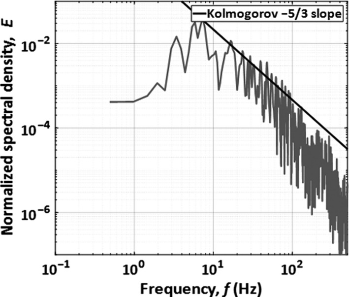
Normalized PSD of residual velocity fluctuations about the moving average

The turbulence intensity, computed from the residual fluctuations about the moving average and averaged across all coughs, was I _ua = 8.9%. As expected, this was very similar to the turbulence intensity computed from the power spectrum, and a value of I _us = 8.4% was calculated (4.6% difference).

3.5. Computational fluid dynamics (CFD) model comparison and analysis

The validity of the numerical simulation was determined by comparing the normalized experimental velocity profiles with those determined computationally (Figure 10). A peak velocity of 0.84 m/s is obtained from the URANS simulation, whereas it is higher in the LES with a value of 0.90 m/s. As expected, the peak velocity obtained from PIV experiments was slightly higher (1.17 m/s), since it was calculated from the instantaneous peak velocity magnitude, whereas the CFD values come from window‐averaged time histories. Both the URANS and LES showed good agreement with the experimental results. The LES may have been a better representation of a realistic cough, but it was substantially more computationally expensive and so may not be practical for some investigations.

Figure 10.

Normalized moving‐averaged velocity time histories (CFD) compared with average PIV instantaneous velocity time history and experimental modeling function V _fit(τ) at x = 1.0 m, on cough jet centerline (y = z = 0)

To gain a better understanding of the decay in V _peak with respect to distance (x) from the source, the instantaneous velocity time histories were extracted along the simulated cough centerline at 0.1‐m intervals, starting at the inlet and extending to x = 1.5 m. The normalized peak velocity,

V _peak‐n, was calculated according to Equation 7,

$$V_{\text{peak}-\mathrm{n}}=\frac{V_{\text{peak}}}{V_{\text{inlet}}}$$ (7)

where V _peak is the peak velocity magnitude observed at each location, and V _inlet is the peak velocity magnitude observed at the inlet, and it is shown vs distance from the inlet in Figure 11.

Figure 11.

Variation of normalized peak velocity and distance from the inlet (CFD)

As examined by Bi, ³⁶ the width of both steady and transient jets increases linearly from the virtual origin, x ₀. The cross‐sectional area of the jet is therefore proportional to (x − x ₀)² so a fitting curve that could be used to predict the decay of the peak velocity observed downstream was determined (Equation 8).

$$V_{\text{peak}-\text{fit}}\left(x-x_0\right)=\frac{A^2}{{\left[\left(x-x_0\right)+A\right]}^2}$$ (8)

where, for LES, A = 0.2810, x ₀ = 0.1098 m, and for URANS, A = 0.2372, x ₀ = 0.1602 m

Using the above equation, and the estimates of peak cough velocity and mouth diameter at the origin from Gupta et al, ²¹ the cough jet velocity will decay to 1% of its initial velocity at x = 115D. Since droplets and droplet nuclei smaller than 10 µm can remain suspended for long periods of time, ³⁶ it is likely that they will be transported by the jet and there is potential for the transmission of viruses at these distances. In practice, the ventilation currents within a room will play a more dominant role at such low velocities.

In this study, the near field was considered to be the region close to the mouth, where the flow field was primarily determined by the initial impulse of the cough, while the far field was defined as the region beyond this where the flow field resembled that of a transient turbulent free jet. In the far field, the velocity time history profiles were similar when normalized using the local peak velocity and timescale. Figure 12A‐D shows that this occurs where x > 0.3 m. When x < 0.3 m, a poor agreement is noticed between the CFD velocity time histories and the average of those obtained experimentally at x = 1.0 m. This means that the present model for far‐field cough flow can be considered valid in the region where x > 15D, based on an estimated mouth opening diameter of 0.0217 m. ²¹ By combining numerical and experimental results, the model can be applied to approximate the cough jet behavior at any location in the far field, although measurements of actual cough flow fields at greater distances than x = 1.0 m (50D) are recommended to confirm the validity.

Figure 12.

Normalized velocity magnitude time histories (A) for x = 0.0‐0.3 m, on cough jet centerline (y = z=0) (LES and ensemble‐averaged PIV), (B) for x = 0.0‐0.3 m, on cough jet centerline (y = z=0) (URANS and ensemble‐averaged PIV), (C) for x = 0.4‐1.5 m, on cough jet centerline (y = z=0) (LES and ensemble‐averaged PIV), and (D) for x = 0.3‐1.5 m, on cough jet centerline (y = z=0) (URANS and ensemble‐averaged PIV)

3.6. Limitations of the present work

The biological air sampling method used in this study was unable to assess the relative significance of far‐field virus transmission. This could mean that that three forced coughing events do not produce a significant quantity of viral droplets, or it is possible that the virus was present but not sampled due to the small area of the sampling cassettes. There is also a possibility that the air sampling method used destroyed the viral particles upon impaction, and, perhaps, in future investigations, aerosols should be sampled for more coughs or an alternative sampling method should be used.

It is possible that the type of viral infection will influence the production of mucous within the lungs and may alter the way a person will cough, such that it may not be accurate to consider all cough jets containing respiratory viruses as being identical. It is also assumed that the trajectory of a natural cough may be different from those studied here since the motion of the head is restricted in the trials. Another assumption used for this investigation is that a forced cough will behave aerodynamically like a naturally occurring cough.

4. CONCLUSIONS

By combining experimental measurements using particle image velocimetry and hot‐wire anemometry and data obtained from previous unsteady Reynolds‐averaged Navier‐Stokes (URANS) and large eddy simulation (LES) CFD simulations, a complete model for the cough centerline peak velocity decay has been developed. Although a high degree of variability is observed between individual coughs, the average profiles are a good representation of the expiratory airflow field produced by a human cough in the region x ≥ 15D. This approximate location can be used to distinguish between near‐field region, where the flow field is primarily governed by the initial cough impulse, and the far‐field region, where the locally scaled velocity time histories collapse upon each other. An average peak velocity of V = 1.17 m/s was observed at the cough center, x = 1.0 m downstream. This is comparable to the velocity determined by the LES (V = 0.90 m/s) and URANS (V = 0.84 m/s), which both used the value of peak velocity at the mouth (x = 0) given by Gupta et al (2009) from their experiments as the initial jet condition. The strong velocities measured provided evidence to dispute previously assumed safe separation distances, and therefore, there is incentive to develop more viable infection prevention methods. The average spread angle of 24° obtained experimentally was comparable to the values previously published for steady free jets, where a spreading angle between 20° and 35° is typically measured. ⁴¹

No statistically significant differences were observed in the velocity or turbulence characteristics between coughs from sick or healthy participants, and evidence was provided to support the claim that velocity data obtained from healthy participants in previous studies can be used to approximate the flow field of coughs from individuals who have been infected with respiratory viruses.

NOMENCLATURE

D

Cough average mouth opening diameter (m)

E

Normalized spectral density

I _ua

Turbulence intensity from moving average (%), $I_{\text{ua}}=\frac{V_{\text{rms}}^{\prime }}{V_{\text{peak}}-V_s}\times 100\%$

I _us

Turbulence intensity from power spectrum (%)

N

Number of samples from hot‐wire anemometer

t

Time (seconds)

t _peak

Time of peak instantaneous velocity for point velocity data (seconds)

Δt

Laser pulse separation time (µs)

u

Axial component of velocity (m/s)

V

2D velocity magnitude (m/s), $V=\sqrt{u^2+v^2}$

v

Vertical component of velocity (m/s)

V _fit

Average velocity magnitude mathematical fitting curve (m/s)

V _norm

Normalized 2D velocity magnitude, $V_{\text{norm}}=\frac{V(t)-V_s}{V_{\text{peak}}-V_s}$

V _peak

Peak 2D velocity magnitude (m/s)

V _peak‐n

Normalized peak 2D velocity magnitude

$V_{\text{rms}}^{\prime }$

Root mean square of velocity fluctuations (m/s)

V_s

Residual velocity when cough enters field of view (m/s)

x

Horizontal direction coordinate (m)

y

Vertical direction coordinate (m)

θ

Jet spread angle (°)

θ ₁

Upper boundary for downward cough angle (°)

θ ₂

Lower boundary for downward cough angle (°)

τ

Dimensionless time, $\tau =\frac{t}{t_{\text{peak}}}$

AUTHOR CONTRIBUTION

The experimental data collection and analysis was performed by Nicholas Dudalski, Ahmed Mohamed, and Eric Savory. The CFD models were developed by Ran Bi, Chao Zhang, and Eric Savory. The biological analysis was performed by Samira Mubareka and her team of researchers at Sunnybrook Research Institute. All authors contributed to and approved the final manuscript.

Dudalski N, Mohamed A, Mubareka S, Bi R, Zhang C, Savory E. Experimental investigation of far‐field human cough airflows from healthy and influenza‐infected subjects. Indoor Air. 2020;30:966–977. 10.1111/ina.12680

REFERENCES

- 1. de Francisco SN, Donadel M, Jit M, Hutubessy R. A systematic review of the social and economic burden of influenza in low‐ and middle‐income countries. Vaccine. 2015;33(48):6537‐6544. [DOI] [PubMed] [Google Scholar]
- 2. Lafond KE, Nair H, Rasooly MH, et al. Global role and burden of influenza in pediatric respiratory hospitalizations, 1982–2012: a systematic analysis. PLoS Medicine. 2016;13(6):e1002060. [DOI] [PMC free article] [PubMed] [Google Scholar]
- 3. Gorbalenya AE, Baker SC, Baric RS, et al. Severe acute respiratory syndrome‐related coronavirus‐The species and its viruses, a statement of the Coronavirus Study Group. bioRxiv. 2020. [Google Scholar]
- 4. World Health Organization . Coronavirus disease 2019 (COVID‐19). Situation report‐23. Reported February 12, 2020.
- 5. Morawska L. Droplet fate in indoor environments, or can we prevent the spread of infection? Indoor Air. 2006;16:335‐347. [DOI] [PubMed] [Google Scholar]
- 6. Xie X, Li Y, Chwang ATY, Ho PL, Seto WH. How far droplets can move in indoor environments – revisiting the wells evaporation‐falling curve. Indoor Air. 2007;17:211‐225. [DOI] [PubMed] [Google Scholar]
- 7. Tellier R. Aerosol transmission of influenza A virus: a review of new studies. J R Soc Interface. 2009;6:6. [DOI] [PMC free article] [PubMed] [Google Scholar]
- 8. Ai ZT, Melikov AK. Airborne spread of expiratory droplet nuclei between the occupants of indoor environments: a review. Indoor Air. 2018;28:500‐524. [DOI] [PubMed] [Google Scholar]
- 9. Yang S, Lee GWM, Chen CM, Wu CC, Yu KP. The size and concentration of droplets generated by coughing in human subjects. J Aerosol Med. 2007;20:484‐494. [DOI] [PubMed] [Google Scholar]
- 10. Xie X, Li Y, Sun H, Liu L. Exhaled droplets due to talking and coughing. J R Soc Interface. 2009;6:S703‐S714. [DOI] [PMC free article] [PubMed] [Google Scholar]
- 11. Morawska L, Johnson GR, Ristovski ZD, et al. Size distribution and sites of origins of droplets expelled from the human respiratory tract during expiratory activities. J Aerosol Sci. 2009;40:256‐269. [Google Scholar]
- 12. Johnson G, Morawska L, Ristovski Z, et al. Modality of human expired aerosol size distributions. J Aerosol Sci. 2011;42:839‐851. [Google Scholar]
- 13. Zayas G, Chiang MC, Wong E, et al. Cough aerosol in healthy participants: fundamental knowledge to optimize droplet‐spread infectious respiratory disease management. BMC Pulm Med. 2012;12:11. [DOI] [PMC free article] [PubMed] [Google Scholar]
- 14. Stelzer‐Braid S, Oliver BG, Blazey AJ, et al. Exhalation of respiratory viruses by breathing, coughing, and talking. J Med Virol. 2009;81(9):1674‐1679. [DOI] [PubMed] [Google Scholar]
- 15. Lindsley WG, Blachere FM, Thewlis RE, et al. Measurements of airborne influenza virus in aerosol particles from human coughs. PLoS ONE. 2010;5:e15100. [DOI] [PMC free article] [PubMed] [Google Scholar]
- 16. Lindsley WG, Blachere FM, Beezhold DH, et al. Viable influenza A virus in airborne particles expelled during coughs versus exhalations. Influenza Other Respir Viruses. 2016;10(5):404‐413. [DOI] [PMC free article] [PubMed] [Google Scholar]
- 17. Mahajan RP, Singh P, Murty GE, Aitkenhead AR. Relationship between expired lung volume, peak flow rate and peak velocity time during a voluntary cough manoeuvre. Br J Anaesth. 1994;72:298‐301. [DOI] [PubMed] [Google Scholar]
- 18. Afshari A, Azadi S, Ebeling T, et al. Evaluation of cough using digital particle image velocimetry. In Conference Proceedings. Second Joint EMBS‐BMES Conference 2002 24th Annual International Conference of the Engineering in Medicine and Biology Society. Annual Fall Meeting of the Biomedical Engineering Society (Cat. No. 02CH37392), IEEE, Piscataway, NJ, pp. 975‐976. [Google Scholar]
- 19. Zhu S, Kato S, Yang J. Study on transport characteristics of saliva droplets produced by coughing in a calm indoor environment. Build Environ. 2006;41:1691‐1702. [Google Scholar]
- 20. Chao C, Wan M, Morawska L, et al. Characterization of expiration air jets and droplet size distributions immediately at the mouth opening. J Aerosol Sci. 2009;40(2):122‐133. [DOI] [PMC free article] [PubMed] [Google Scholar]
- 21. Gupta JK, Lin CH, Chen Q. Flow dynamics and characterization of a cough. Indoor Air. 2009;19:517‐525. [DOI] [PubMed] [Google Scholar]
- 22. Tang JW, Liebner TJ, Craven BA, Settles GS. A Schlieren optical study of the human cough with and without wearing masks for aerosol infection control. J R Soc Interface. 2009;6(Suppl. 6):S727‐S736. [DOI] [PMC free article] [PubMed] [Google Scholar]
- 23. VanSciver M, Miller S, Hertzberg J. Particle image velocimetry of human cough. Aerosol Sci Technol. 2011;45:415‐422. [Google Scholar]
- 24. Nishimura H, Sakata S, Kaga A. A new methodology for studying dynamics of aerosol particles in sneeze and cough using a digital high‐vision, high‐speed video system and vector analyses. PLoS ONE. 2013;8(11):e80244. [DOI] [PMC free article] [PubMed] [Google Scholar]
- 25. Bourouiba L, Dehandschoewercker E, Bush JW. Violent expiratory events: on coughing and sneezing. J Fluid Mech. 2014;745:537‐563. [Google Scholar]
- 26. Savory E, Lin WE, Blackman K, et al. Western cold and flu (WeCoF) aerosol study preliminary results. BMC Res Notes. 2014;7(1):563. [DOI] [PMC free article] [PubMed] [Google Scholar]
- 27. Booth TF, Kournikakis B, Bastien N, et al. Detection of airborne severe acute respiratory syndrome (SARS) coronavirus and environmental contamination in SARS outbreak units. J Infect Dis. 2005;191(9):1472‐1477. [DOI] [PMC free article] [PubMed] [Google Scholar]
- 28. Blachere FM, Lindsley WG, Pearce TA, et al. Measurement of airborne influenza virus in a hospital emergency department. Clin Infect Dis. 2009;48(4):438‐440. [DOI] [PubMed] [Google Scholar]
- 29. Yang W, Elankumaran S, Marr LC. Concentrations and size distributions of airborne influenza A viruses measured indoors at a health centre, a day‐care centre and on aeroplanes. J R Soc Interface. 2011;8(61):1176‐1184. [DOI] [PMC free article] [PubMed] [Google Scholar]
- 30. Lowen AC, Mubareka S, Steel J, Palese P. Influenza virus transmission is dependent on relative humidity and temperature. PLoS Pathog. 2007;3(10):e151. [DOI] [PMC free article] [PubMed] [Google Scholar]
- 31. Lowen AC, Mubareka S, Steel J, Palese P. High temperature (30°C) blocks aerosol but not contact transmission of influenza virus. J Virol. 2008;82(11):5650‐5652. [DOI] [PMC free article] [PubMed] [Google Scholar]
- 32. Steel J, Lowen AC, Mubareka S, Palese P. Transmission of influenza virus in a mammalian host is increased by PB2 amino acids 627K or 627E/701N. PLoS Pathog. 2009;5(1):e1000252. [DOI] [PMC free article] [PubMed] [Google Scholar]
- 33. Mubareka S, Lowen AC, Steel J, Coates AL, Garcia‐Sastre A, Palese P. Transmission of influenza virus via aerosols and fomites in the guinea pig model. J Infect Dis. 2009;199(6):858‐865. [DOI] [PMC free article] [PubMed] [Google Scholar]
- 34. Deller B, Stolarsky G, Tietjen L. Preventing the transmission of avian or pandemic Influenza in health care facilities with limited resources: Learning resource package. Jhpiego: An affiliate of John Hopkins University. 2008;2:5. [Google Scholar]
- 35. Kennamer M. Infection Control for Health Care Providers. Albany: Thomson Delmar Learning; 2007;79‐85. [Google Scholar]
- 36. Bi R. A numerical investigation of human cough jet development and droplet dispersion. M.E.Sc. Thesis, Dept. Mech. & Matls. Eng., University of Western Ontario, London, Canada; 2018. [Google Scholar]
- 37. Yan J, Grantham M, Pantelic J, et al. Infectious virus in exhaled breath of symptomatic seasonal influenza cases from a college community. Proc Natl Acad Sci. 2018;115(5):1081‐1086. [DOI] [PMC free article] [PubMed] [Google Scholar]
- 38. Mohamed A. Experimental measurements of far‐field cough airflows produced by healthy and Influenza infected human subjects. M.E.Sc. Thesis, Dept. Mech. & Matls. Eng., University of Western Ontario, London, Canada; 2017. [Google Scholar]
- 39. Coleman HW, Steele WG. Experimentation, Validation, and Uncertainty Analysis for Engineers, 3rd ed. Hoboken, NJ: John Wiley & Sons, Inc.; 2009. [Google Scholar]
- 40. Verrault D, Moineau S, Duchaine C. Methods for sampling of airborne viruses. Microbiol Mol Biol Rev. 2008;72(3):413‐444. [DOI] [PMC free article] [PubMed] [Google Scholar]
- 41. Ball CG, Fellouah H, Pollard A. The flow field in turbulent round free jets. Prog Aerospace Sci. 2012;50:1‐26. [Google Scholar]