

Graphical abstract
Figure 1. FHFAG system. Ultra-precision machining for large aperture optical elements is becoming more and more important with the development of modern industry such as giant space telescope and large laser equipment. This paper is a critical paper which can take FHFAG in to the aforementioned practice as it studied the removal function theoretically and experimentally.

Keywords: Removal function, Fluid hydrodynamic, Fixed abrasive grinding, Fully coupled flow deformation model
Highlights
-
•
Building the fully coupled model to analyze liquid film characteristics.
-
•
Analysis of the removal mechanism of hard and brittle materials.
-
•
Building the relationship between the cutting depth and the concrete removal volume.
-
•
Machining experiments has been done to verify the correctness of the theoretical model.
-
•
Planarization processing experiment demonstrated practicability of the removal function.
Abstract
Fluid hydrodynamic fixed abrasive grinding (FHFAG) is now evolving into a promising finishing method underpinning the major advances across grinding and lapping sciences. While the advances have been startling, the key unmet challenge to date is the theoretical basis of removal function. Here, we approach this challenge by presenting a fully coupled flow deformation model. Given the separation function on microchannel from the grits fixed on the grinding pad, hydrodynamic pressure distribution with many dynamic pressure peaks and basic film thickness can be described theoretically. Combining with primary material removal mechanism the removal function of FHFAG was achieved. The experimental results showed a strong agreement with the prediction removal function model and its practicability has also been verified.
Introduction
Large aperture optical elements are attractive for many applications due to their superior properties [1], [2], [3], Machining of these hard and brittle materials has gained significant importance over decades [4]. Several modern processing methods have emerged to approach across the lapping and polishing manufacturing sciences. At the low frequency error scale, methods such as computer control optical polishing [5], [6] (CCOS) and bonnet polishing [7] (BP) can remove the profile error of the workpiece efficiently. While at the high frequency error scale, methods such as magneto rheological finishing [8], [9] (MRF) and ion beam figuring [10] (IBF) are taking hold in precision finishing stage. Generally, the combination of the methods mentioned above can approach to a highly qualified optical element [11]. A grand challenge in this area is to perform such processing both efficiently and precisely. Here, we present a new processing method called fluid hydrodynamic fixed abrasive grinding [12] (FHFAG, Fig. 1). Specifically, a fixed abrasive grinding pad has been used in a CCOS performance. More interestingly, we supply the grinding fluid which is deionized water from the center of the grinding pad. Key advances have emerged by a consideration of the hydrodynamic action of the liquid film between the grinding pad and workpiece. The liquid film in the microchannel separates the grinding tool and the optic elements that the grits, fixed on the grinding pad, will cut in the workpiece partially instead of totally. Therefore, the cutting depth can be changed by controlling the thickness and dynamic pressure distribution of the liquid film. This constitutes a totally novel perspective for utilizing liquid film in microchannel compared with traditional methods [13], [14]. While the advances have been startling, the key unmet challenge to date is the theoretical basis of removal function.
Fig. 1.

FHFAG system.
Fluid dynamic pressure distribution in microchannel has been extensively investigated over the past several decades [15], [16]. Continuum theory is applicable to single-phase liquid flow in microchannel, which implies that the equations developed for macroscale applications, such as the Reynolds equation, will be applicable to even small channels [17], [18]. However, given that the separation function of the grits stands in the path of the flow, the real fluid flow situation cannot be described by full film regime theoretical predictions [18], [19]. Besides, different deflections will appear near the different dynamic pressure peaks. The deflection will, in turn, affect the dynamic pressure distribution.
The partial film regime theory was employed in elastohydrodynamic lubrication firstly. The inclusion of surface irregularities in lubrication analysis can be traced back to the 1960s [20], [21], [22], in which the roughness is modeled as sinusoidal or saw-tooth waviness. Subsequently, Tseng and Saibel [23] introduced the stochastic concept based on random surface roughness analysis on lubrication. However, their method deals with surfaces with one-dimensional transverse roughness only. The stochastic model has been revived by Christensen and colleagues [24], [25], [26], [27], [28] in studying the lubrication process between rigid surfaces containing surface roughness modeled as ridges oriented transversely or longitudinally.
As described above, although FHFAG has been proven to be practical by a preliminary experiment, there is still no appropriate theoretical model to precisely describe the complicated flow field and contact situation. Here, we present a full coupling model which considers an advanced partial film regime theory and the deformation effect. Based on this model, a decisive removal function shape can be achieved by combination with primary material removal mechanism. A stable double peaks shape removal function was proved by both of the theoretical and experimental results.
Material and methods
Analysis for the liquid film characteristics
As shown in Fig. 1, the key point of FHFAG is the utilization of the liquid film. The system comprises some rules and assumptions: Using the exposed height maximum depth of the abrasive grinding polishing pad as the grinding state; the sum of the liquid film thickness and the maximum grinding depth is determined by the determined grinding pad; the polishing load is shared by the liquid film’s buoyancy and the contact force of the abrasive. The working load is shared by the contact force from the grits’ cutting action and buoyance from the fluid dynamic pressure. Besides, the basic film thickness distribution is the factor to decide the machining precision. Therefore, the liquid dynamic pressure distribution and basic film thickness distribution is the main research object for analysis for the liquid film characteristics.
The fluid hydrodynamic phenomenon in FHFAG is the central scientific problem. At the same time, it’s a very complicate system coupled by input parameters, procedural parameters and output parameters as shown in Fig. 2.
Fig. 2.

Basic logical relationships in FHFAG.
Basic arithmetic relations in Fig. 2 are presented in Equation (1) and Equation (2).
| (1) |
| (2) |
At first, the contact force (Fc) carries working load (Pload) alone when the fluid is not filled in the microchannel. Fc is the summation of all the grits’ normal cutting force which is decided by the cutting depth (hcut) for grits. So, the original thickness distribution can be achieved from pad’s surface topography and Pload which can both be regarded as the input parameters. When fluid comes into the microchannel and form a liquid film, the buoyancy force (P) which is the integral value in the working area will play an important role to share the carrying responsibility. Based on Equation (2), in order to reach a new balance, the channel will expand to decrease the Fc by reducing the hcut. On the other hand, the integrated film thickness (h) distribution will affect the dynamic pressure distribution conversely. Above all, the thickness of the film will get a final distribution to make the whole system get balanced.
Topography of the fixed abrasive grinding pad
The model of the grinding pad’s topography comprises the premise of establishing the fully coupling model. The height data of the grinding surface can describe the original contact situation precisely. A body-centered cubic cell model is applied to summarize the grinding pad’s topography. Spherical shape grits generate on the nodes of the cube. Under the condition of noninterference, the grits can vibrate randomly around their own corner.
Grains that shape on the pad tend to be cubic, cub octahedron, and spherical. The cubic and cub octahedron CeO2 grains produced by the regular method can easily scratch the glass and damage the subsurface. The spherical grains produced by the detonation technique exhibit better performance. For the universality of the method, all grit types in this research are supposed to be spherical. In fact, it is reasonable to make this simplification because the grains have a great negative rake when cutting. In the actual production, the particular level of CeO2 powder grits size can be obtained from the standard sieve’s screening. The grits size can be controlled in a certain range. However, the specific size for a single grit is not definite, and thus the central-limit theorem of statistics is used in the prediction of the particle size distribution. The grits’ size follows a Gaussian distribution as shown in Fig. 3a.
Fig. 3.

Establishment of the mathematical model for the grinding pad’s surface topography. (a) Grits size Gaussian distribution diagram. The grits follow Gaussian distributions whose size was controlled by a standard sieve between interval [dgmin, dgmax]. The expectancy was μg, and the variance was σg2. (b) Body cubic cell model. There are two grits in one cell on average. The volume concentration of the pad of the sample from Saint-Gobain is approximately 15.52%. Sg can be calculated as 14.87 μm from Equation (8). (c) Grit random offset schematic diagram. The offsets for direction X, Y, and Z are σx, σy, and σz, respectively, which should follow Gaussian distributions whose mathematical expectation is 0 and variance is Sg/6. (d) Grit number schematic diagram.
Equation (3) presents its probability density function. The size is controlled by a standard sieve between interval [dgmin, dgmax], and the expectancy is μg. Variance is σg2 represented by Equation (4) and Equation (5)
| (3) |
| (4) |
| (5) |
The establishment of the model can be summarized by Fig. 4. The first step is arranging the original grid point in an orderly manner. Mean spacing between two adjacent grits is the key factor. A body-centered cubic cell model (Fig. 3b) is applied in this research. It can be clearly seen that Sg, which is the length of the cubic edge, can be regarded as the spacing. It is related to the grits’ size and volume concentration of the pad.
| (6) |
| (7) |
where is the grits’ volume in a cubic cell; is the cubic cell’ volume; and is the average diameter of the grits. Therefore, (the volume concentration of the grits is 15.52%) is the ratio of and . The average diameter of the grits is the expectancy of the grits which means. Sg can be shown in Equation (8).
| (8) |
Fig. 4.

Mathematical model for the grinding pad’s surface topography. (a) Grid points prior to randomization. (b) Grid points after randomize. (c) Spherical grains generated around the grid points. (d) Sampling of height data in cylindrical coordinates.
In the real situation, the particles could not remain in the corners uniformly. Its central positions need random migration processing. The offsets for direction X, Y, and Z are σx, σy, and σz, respectively, which should follow a Gaussian distribution whose mathematical expectation is 0 and variance is Sg/6 (Fig. 3d). The grit whose sequence number is i, j, k is numbered in direction X, Y, Z as ijk, and the central position is (xijk, yijk, zijk) named Gijk (Fig. 3c). Equation (9) presents the final central position for the grits.
| (9) |
Fig. 4c shows the generation of spherical grits with different diameters. Sampling the height data in cylindrical coordinates makes it easier to apply to the annular research area.
In order to verify the correctness of this method, a real grinding pad was observed under KEYENCE VHX-1000.
The height data of the pad are obtained after processing the image of the real pad surface (Fig. 5a, 5c, 5d). Correlation coefficient was employed here to measure the degree of similarity between simulation results and the real pad. Finally, the correlation coefficient was 0.901 which demonstrated the statistical results of the simulation result and real pad (Fig. 5b) have good agreement that the simulation data are reliable, and can be used in the fully coupled model.
Fig. 5.

Grinding pad surface. (a) Real surface of W14 pad. Grits fixed on the pad are CeO2, with a diameter ranging from 10 μm to 14 μm. (b) Comparison between the real pad’s blade height distribution and simulation result. (c) Part of the W14 pad real surface with the organism being dyed. The pad organism was made of polyurethane, and its color was close to the particles. For convenience of handling and analyzing the image, a dyeing process was performed on the organism with black ink. (d) Gray scale image of Fig. c. Gray level is ranges from 0 to 255 s and the color changing from black to white as the number becomes larger. Each single grey level could correspond to a certain blade height.
Fully coupled model of the microchannel
The actual situation in the microchannel is very complex in the FHFAG system. The basic hypothesis of FHFAG is the buoyancy from the dynamic pressure and the contact force to carry working load. The pad organism is made of polyurethane. A certain degree of deformation will appear on the pad due to the stress from the dynamic pressure. Workpiece (e.g. fused silica glass) can be regarded as a rigid body because of its much greater hardness compared to that of the pad. Therefore, fluid–structure interaction relationships exist among numerous parameters.
Based on fluid mechanics theory and the special condition in the FHFAG system, a reformed Reynolds equation for two-dimensional pressure distributions is utilized here. Considering that the contact area is toroidal, [29] and the coefficient Re is supposed to be less than the critical one.
| (10) |
where ρ, and η are the density and viscosity of the grinding liquid respectively; ω is the rotation speed of the grinding pad; p is the dynamic pressure, which could also be also noted as p(r, θ); and H(r, θ) is the film thickness.
Equation (10) is the mathematical presentation of the fully coupled model for the FHFAG system. Specially, it’s P’s implicit function on r and θ. The deformation matrix concept and the finite difference method have been used in decoupling the mathematical model.
Particularity of FHFAG system is utilizing the coupling relationship among some parameters. The carrying capacity will be changed because of the changing dynamic pressure distribution. In addition, the pad’s deformation distribution will also be changed. Then, the film thickness must be updated according to the corresponding dynamic pressure distribution, which is the combination of the basic thickness of film and deformation of the pad, as shown in Equation (11).
| (11) |
The first part can be deduced by the grinding pad’s surface topography and cutting depth of grits as presented in Equation (12).
| (12) |
where hCYL(r, θ) is the grinding pad’s surface height of point(r, θ); Max(hCYL) is the maximum exposing height of the grinding pad surface; and hcut is the maximum cutting depth.
In actual production, the pressure peaks appear closed to the grits, which affects the pressure peaks’ distribution. Therefore, the deformation of the grinding pad caused by the pressure peaks cannot be neglected. The stress on the grinding pad can be regarded as Hertz stress [30], [31], and deformation can be deduced as Equation (13).
| (13) |
where δ(r, θ) is the deformation of point (r, θ); P(m, n) is the pressure on point (m, n); and E is the elastic-modulus of the pad.
Equation (10) is a partial differential equation of second order about P. In this research, the model is discretized and approximated to a polar-grid by applying a second-order accurate central difference in space [19].
δ(r, θ) is achieved by using the deformation matrix method because it cannot be integrated (see Supplementary 2 for details). An underrelaxation scheme is applied for approaching the true solution of the discretized equation (see Supplementary 3 for details). The working condition discussed in this paper is a ring-shaped grinding pad. The pad rotates at a certain speed and the fluid is injected from the central hole by a given pressure. Then, the fluid is discharged naturally from the pad’s edge by atmospheric pressure. Fig. 6a shows the calculation results of this model.
Fig. 6.

Calculation results for fully coupled model. (a) Fluid dynamic pressure distribution of the contact area. The input pressure is 0.3Mpa, working load is 120 N, and rotary speed of the grinding pad is 4000 rpm. Grits being fixed on the pad are diamond abrasive with a size of W28 (b) Generalized dynamic pressure along the diameter direction. The input pressure is 0.3Mpa; the dynamic pressure value in the picture is the average value of the pressure in the same radius. (c) Basic thickness of the microchannel and the buoyancy force by different velocity speed. The input pressure is 0.3Mpa.
The ridges of the dynamic pressure are caused by the dynamic grooves on the grinding pad. The maximum value is approximately 40Mpa, which can supply an efficient buoyancy force. The dynamic pressure peaks are caused by the grits. The tiny wedge gaps between the workpiece and different grits can make different pressure peaks. In fact, the cutting action of the grits can cut the continuity of the fluid, which is detrimental to the stability of the balanced state. Therefore, in another side, the dynamic grooves can strengthen the system’s stability. Fig. 6b shows the comparison result for different rotation speeds. The squeezing effect from the dynamic pressure distribution will lead to a certain degree of deformation of the substrate material. Poisson's effect can be used here to explain the waves; such as pressure distributions along the diameter direction. Moreover, the average pressure is increasing with the rising of the grinding tool’s rotation speed, which is fully compliant with fluid mechanism principle. The basic thickness of the microchannel means where the microchannel has no grits (Fig. 1). The dynamic pressure and the basic thickness will achieve a balanced state after the decoupling operation for the model. The cutting depth for each single grit can be obtained based on the balanced microchannel. The buoyancy force is the summation of the dynamic pressure. The buoyancy force and the contact force bear the working load. Both the basic film thickness and the buoyancy force have a positive relationship with grinding tool’s rotary speed (Fig. 6c).
Remove function for fused silica glass
Fused silica glass has some superior properties, such as high hardness and strength at elevated temperatures, chemical stability, low friction, and high wear resistance that it can be used as the material of large aperture optical elements. In this part, we make it as the workpiece material.
Generally, point of a plastic removal region for hard and brittle material is acceptable due to its hard and brittle property. However, the plastic removal region is so narrow that the plastic removal effect could be regarded as a planarization process without an actual material removal effect. Therefore, the brittle removal effect is studied in this research. Brittle fracture is the removal mechanism for hard and brittle material like fused silica glass. However, the relation between a chip’s volume and the cutting parameters still remains unclear. In this research, the relation is investigated from a geometrical perspective (Fig. 7).
Fig. 7.

Idealized lateral crack system. (a) The contact at load Pload leads to a crack of characteristic radius ch at depth below the surface. A scratching zone which presented as area 1 can be achieved. The plastic zone which is area 2 supports the grit. The contact angle is 2ψ, and the contact radius is a, and extends outwards to a radius ch. A material removal zone which is area 3 will drop off. (b) The overlapping of two grains.
An idealized lateral crack system [32] is cited here to characterize the brittle removal effect as shown in Fig. 7a. The penny-like lateral crack will extend to the surface and be removed when the grit moves away. All of the geometric elements in Fig. 7 could be obtained from the cutting depth hcut, and the physical properties of the glass itself. Therefore, the removal volume in unit time can be attained by Equation (14):
| (14) |
where S is the semi elliptic cross-sectional area, and is also an explicit function of hcut; and v is the linear velocity of the correspondent grit.
hcut and dg are the cutting parameters, except the glass’s physical properties. The semi elliptic cross-sectional area S in Equation (14) is the key factor to solve the problem. Once the grit moves, the lateral crack will be initiated, and it will propagate on the plane parallel to the substrate surface. The propagation of the cracks is controlled by tensile stresses. Evans et al [33], [34]. showed that the tensile stresses that cause the lateral fracture are at a maximum near the elastic–plastic boundary. Thus, it has been concluded that the depth h at which lateral cracks initiate is equal to the depth of the plastic zone ch. Equation (15) is based on elliptical area formula:
| (15) |
The indention length a, and the radius of the plastically deformed zone ch can be correlated via the Hill model of the expanding cavity in a perfect plastic material [35].
| (16) |
where m is a dimensionless constant, for which more recent research suggests m = 0.43, E, H, and μ is Young modulus, Vickers hardness, and Poisson's ratio, respectively for material. αk is a constant related with m as presented in Equation (17).
| (17) |
The equilibrium crack size cL can be expressed as a function of the applied load [33].
| (18) |
where E is Young modulus; and Kc is the fracture toughness of the substrate. The final removal function can be achieved as Equation (19).
| (19) |
φ, and P is decided by the local grit’s radius and local cutting depth presented by Equation (20) and Equation (21), respectively. In other words, the liquid film’s thickness distribution from the coupling model has decided the removal volume in unit time.
| (20) |
| (21) |
Combining the cutting depth distribution proposed previously and the removal volume model, the removal volume for a specific grit can be achieved. So, the accurate removal function is obtained after reasonable trajectory superposition processing. In order to compare with the experiment results, fixed point grinding processing has been calculated according to the removal function. Fig. 8 presents the final removal function for different working parameters (see Supplementary 4 for details). Values have been normalized for the convenience of observation and comparison with the experimental results.
Fig. 8.

Removal function under different working parameters for single point model. Each of the panel is the calculation result corresponding to the experiment number in Supplementary 4, Tab. S2. The scale bar on the right of the panels are the normalized values.
As shown in Fig. 8, the removal function for single spot is quite different with the traditional Preston equation method. A double peak shape appears along the radius direction.
Experimental equipment and experiment design
In order to verify the matching model, our experiment is performed in a three-axis NC grinding machine tool which is designed specifically for FHFAG as shown in Fig. 9. The whole system is fixed on the machine bed (7, Marble bed, Jinan River Trade and Industry Co. Ltd). A suspension system (1, DSBC-PPS, Festo) can balance the gravity of center outlet spindle (2, GS120, Taiwan Honghai Industry Co. Ltd) whose rotation speed ranging from 0 rpm to 12000 rpm, and the grinding tool (3) zoomed in by Fig. 9b. At the same time, it can also supply the working load ranging from 0 to 300 N on the workpiece (5, JC-Z02, China Building Material Academy). The Water tank (4) can storage the deionized water acting as the grinding liquid supplied from a water supply system (8) with original pressure 0.3Mpa. The water tank is fixed on a working stage which carried by the servo system (6). A temperature regulation system is used to control the liquid temperature at 20℃.
Fig. 9.
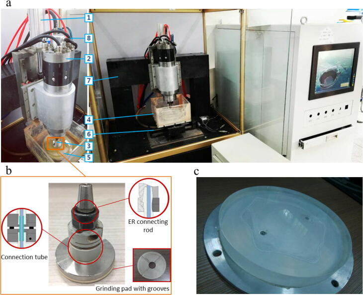
Experimental arrangement. (a) Scheme of the three-axis NC (b) Grinding tool. (c) Workpiece.
As shown in Fig. 9b, to strengthen the fluid dynamic pressure, dynamic grooves are made on the grinding pad (R1 = 20 mm, R2 = 5 mm). The substrate material of the pad is polyurethane (E = 85.3*10^6 Pa, μ = 0.4, ρ = 0.71*10^3Kg/m3). Grains being fixed on the pad are CeO2 abrasive with a size of W28. Before the experiments, our fused silica glass (E = 7.25*10^10 Pa, μ = 0.17, ρ = 2.2*10^3 Kg/m3) as shown in Fig. 9c is preprocessed to have a mirror-like surface. The surface roughness and the topography are measured before and after the machining. The instruments used is NANOVEA ST400 3D non-contact contour meter. A group of fixed-point grinding experiments have been performed. Working parameters being controlled in this experiment are designed the same as our theoretical calculation (see Supplementary 4 for details).
Results and discussion
Investigations were carried out into the comparison of experiment results and calculation results as shown in Fig. 10. The grinding experiment is a fixed-point process without the superposition of a trajectory and some other smooth process. Therefore, surface roughness is not regarded as the evaluation parameter in this experiment. All the data in the figure were normalized.
Fig. 10.

Comparison between experimental results and calculation results for fixed single point experiments. Each of the panel is the calculation result corresponding to the experiment number in Supplementary 4, Tab. S2. All the values have been normalized by the experiment results value of No. L23.
After the normalization, the experimental results can meet the calculation very well from the shape. The calculation values are a little greater than the experimental results. This can be explained by the wear condition of the grains in the experimental situation. In our calculation, the wear situation was not being taken into consideration. Correlation coefficient was employed here to measure the degree of similarity between experimental and calculation results. Finally, the correlation coefficient was 0.714 ± 0.102 which demonstrated the calculation model for the remove function is correct.
Fig. 10 presents the removal function at different rotary speeds and different working load. Interestingly, MRR at 2000 rpm is greater than at any other speed, which means that MRR possesses a parabolic relationship with rotational speed. At first, MRR increase with the increment of rotary speed; a peak is then achieved, followed by a decrease. Generally, MRR is positively correlated to the linear speed of the grits in the grinding process. However, the complex fully coupled model makes this occur in fluid hydrodynamic fixed abrasive grinding. Both the buoyancy force and basic film thickness have a positive relationship with rotary speed. Initially, carrying capacity is limited due to small speed, and the thickness of the film decreases to balance the constant working load by increasing the dynamic pressure and contact force. Therefore, rotary speed played a more important role in the process. However, the dynamic pressure would increase sharply when the speed reached a certain critical speed due to the effect from the dynamic grooves on the grinding pad. The dynamic pressure would raise the grinding pad, and the cutting depth for a single particle would decrease sharply. In addition, fewer grits could touch the workpiece surface. In this case, the increment of pressure played a more essential role. Therefore, the rotary speed affected the removal efficiency through a parabolic shape. The peak point can be considered as the critical speed.
Furthermore, the double peaks shape removal function appears clearly in the theoretical and experimental results. Specially, the removal value is very small when the speed is 4000 rpm. Theoretically, there would be no removal volume according to the model proposed above. The grits can contact the glass’s surface before the whole system reaches a balanced state. The contact would also make some scratches. The strong agreement between the experimental results and the theoretical results proves that the coupled model can accurately describe the complex situation in the microchannel.
Surface profile grinding experiments
As has been aforementioned, the purpose of FHFAG is substantially improving both accuracy and efficiency. In this surface profile experiment, the FHFAG has been used in a planarization processing for the workpiece.
The main purpose of planarization processing is removal the materials between the original and target size which can be defined as ΔE (x, y). The mathematical model of this processing can be depicted as the convolution of the removal function which can be defined as M (x, y) and the dwell time which can be defined as T (x, y) at some specific points. M (x, y) has been theoretically achieved and experimentally identified. T (x, y) needs a deconvolution calculation between ΔE (x, y) and M (x, y). Several kinds of mathematical models have had been developed as the matter of trajectory of the machining tool. As the T (x, y) research was not the main point of this paper, here we employed a general model depicted as regularization method of matrix equation [36].
The planarization processing area was a 100 × 100 mm square. The removal target was a 10 μm down edge processing error coming from the pre-machining process. The removal function employed here is planetary motion removal function being composed by the fixed-point removal function aforementioned. The speed ratio of autobiography and revolution was −10 and the eccentricity ratio was 0.9. Other working parameters being controlled in this experiment has been shown in Supplementary Table S3. The experiment results are shown in Fig. 11.
Fig. 11.

Surface profile grinding experiment results. The 3D profiles were measured by NANOVEA ST400 3D non-contact contour meter, and the step size were both 2.5 μm along x and y axis. Panel (a) (c) and (e) were the original profiles of #1 #2 and #3 pieces. Panel (b) (d) and (f) were the one-round FHFAG processed profiles of #1 #2 and #3 pieces. (g) is the material remove rate (MRR) in surface. Panel (h) and (g) show the PV an RMS statistics before and after the processing.
The results in Fig. 11h and Fig. 11i have shown a strong PV and RMS convergence function over the whole area by one-round FHFAG processing. The deference of the convergence rate came from the different working parameters. Fig. 11g showed a great material removal rate. The MRR can be 23.36 mm3/min which can surpass the limited MRR (6.81 mm3/min) of bonnet polishing processing method at the similar working parameters. The results of the profile grinding experiment have verified the PV and RMS convergence function and the high MRR ability of FHFAG.
Based on the experiment results, another planarization processing experiment was performed. The basic frame was grinding the surface from the low quality to high quality by several rounds with different working parameters. Here, we performed the planarization processing for three rounds employed the working parameters of L1 L2 and L3 in Fig. 11 sequentially. The processing time for each round was 33 min, 25 min and 8 min respectively. The experiment results have been shown in Fig. 12.
Fig. 12.

Planarization processing experiment results. The 3D profiles were measured by NANOVEA ST400 3D non-contact contour meter, and the step size were both 2.5 μm along x and y axis. Panel (a) (b) (c) and (e) are the surface profile for the original, 1 round processed, 2 rounds processed and 3 rounds processed grinding. Panel (e) and (f) are the PV and RMS convergence statistics.
PV for Fig. 12a, b, c and d were 18.72 μm, 8.77 μm, 5.17 μm and 3.82 μm respectively. RMS for Fig. 12a, b, c and d were 2.44 μm, 1.34 μm, 0.85 μm and 0.46 μm. these results can verify the processing convergence function of FHFAG. Besides, the total processing time of the three rounds was 68 min that the average MRR was 13.32 mm3/min without replacing the grinding pad (W28). The results demonstrated a controllable planarization processing with relatively high working quality and high efficiency which can verified the practicability of the removal function for FHFAG.
Conclusion
The fluid hydrodynamic fixed abrasive grinding described here constitutes a novel processing method for large optic elements. The basic concept is controlling the cutting depth for all of the grains by operating the fluid film. The experiment has demonstrated that the grinding pad can float on the film steadily, and the whole system can reach a balanced state. However, the actual situation of the film in the microchannel, which is the key to identifying the mechanism, is quite complex. Mutual coupling relations exist among several important quantities. The mathematical analysis performed for the entire machine process demonstrates that it is scientifically credible.
In summary, a fully coupled model that elucidates the fluid film’s actual complex situation and the grains’ cutting condition is proposed in this research. The grains fixed on the grinding pad have a strong segmentation effect on the fluid film. Specifically, the pressure peaks around the grits are harmful to the formation of static fluid film. However, the dynamic grooves on the grinding pad improve the system’s stability so that the coefficient Re can be supposed to be less than the critical one. The squeezing effect from the dynamic pressure distribution will lead to a certain degree of deformation of the substrate material. The deformation is polycyclic due to Poisson's effect. So, pressure distributions along the diameter direction appear as wave propagation. The combination of polycyclic deformation and grits’ working speed difference at different positions makes a double peaks shape removal function. The strong agreement between the experimental results and the theoretical results fully demonstrates that the prediction about the complex situation in the microchannel is reliable. Finally, the three-round planarization processing experiment with relatively high machining quality and efficiency demonstrated practicability of the removal function for FHFAG.
Declaration of Competing Interest
The authors declared that there is no conflict of interest.
Acknowledgments
This work is mainly supported by the National Science and Technology Major Project of the Ministry of Science and Technology of China (Grant No. 2013ZX04001000-207).
Footnotes
Peer review under responsibility of Cairo University.
Supplementary data to this article can be found online at https://doi.org/10.1016/j.jare.2020.05.023.
Appendix A. Supplementary material
The following are the Supplementary data to this article:
References
- 1.Betti R., Hurricane O. Inertial-confinement fusion with lasers. Nat Phys. 2016;12:435. [Google Scholar]
- 2.L.D. Feinberg, Engineering history of the james webb space telescope (jwst) optical telescope element, DOI (2018).
- 3.R.A. Hyde, Eyeglass. 1. Very large aperture diffractive telescopes, Appl. Opt., 38 (1999) 4198-4212. [DOI] [PubMed]
- 4.Dandekar C.R., Shin Y.C. Modeling of machining of composite materials: a review. Int. J. Mach. Tool Manu. 2012;57:102–121. [Google Scholar]
- 5.Cheng H.-B., Feng Z.-J., Cheng K., Wang Y.-W. Design of a six-axis high precision machine tool and its application in machining aspherical optical mirrors. Int. J. Mach. Tool Manu. 2005;45:1085–1094. [Google Scholar]
- 6.Cheung C.F., Kong L.B., Ho L.T., To S. Modelling and simulation of structure surface generation using computer controlled ultra-precision polishing. Precis Eng. 2011;35:574–590. [Google Scholar]
- 7.Zeng S., Blunt L. Experimental investigation and analytical modelling of the effects of process parameters on material removal rate for bonnet polishing of cobalt chrome alloy. Precis Eng. 2014;38:348–355. [Google Scholar]
- 8.Iqbal F., Jha S. Experimental investigations into transient roughness reduction in ball-end magneto-rheological finishing process. Mater Manuf Processes. 2018;1–8 [Google Scholar]
- 9.Singh A.K., Jha S., Pandey P.M. Nanofinishing of A Typical 3D Ferromagnetic Workpiece Using Ball end Magnetorheological Finishing Process. Int J Mach Tool Manu. 2012;63:21–31. [Google Scholar]
- 10.Bauer J., Frost F., Arnold T. Reactive ion beam figuring of optical aluminium surfaces. J Phys D-Appl Phys. 2017;50 [Google Scholar]
- 11.Fang F.Z., Zhang X.D., Weckenmann A., Zhang G.X., Evans C. Manufacturing and measurement of freeform optics. CIRP Ann. 2013;62:823–846. [Google Scholar]
- 12.Liu P., Lin B., Zhang X., Li Y. Fluid hydrodynamic fixed abrasive grinding based on a small tool. Appl Optics. 2017;56:1453–1459. [Google Scholar]
- 13.Liu H., Xu H., Ellison P.J., Jin Z. Application of computational fluid dynamics and fluid–structure interaction method to the lubrication study of a rotor–bearing system. Tribol Lett. 2010;38:325–336. [Google Scholar]
- 14.C. Hall, S.L. Dixon, Fluid mechanics and thermodynamics of turbomachinery, Butterworth-Heinemann2013.
- 15.Campbell I., Turner J. Turbulent mixing between fluids with different viscosities. Nature. 1985;313:39. [Google Scholar]
- 16.Amini H., Sollier E., Masaeli M., Xie Y., Ganapathysubramanian B., Stone H.A. Engineering fluid flow using sequenced microstructures. Nat Commun. 2013;4:1826. doi: 10.1038/ncomms2841. [DOI] [PubMed] [Google Scholar]
- 17.Ho C.-M., Tai Y.-C. Micro-electro-mechanical-systems (MEMS) and fluid flows. Annu Rev Fluid Mech. 1998;30:579–612. [Google Scholar]
- 18.Stroock A.D., Dertinger S.K., Ajdari A., Mezić I., Stone H.A., Whitesides G.M. Chaotic mixer for microchannels. Science. 2002;295:647–651. doi: 10.1126/science.1066238. [DOI] [PubMed] [Google Scholar]
- 19.Liu P., Lin B., Li Y., Zhang X., Fei J. Liquid film characteristic in fluid hydrodynamic fixed abrasive grinding. Int J Adv Manuf Technol. 2018;96:4205–4214. [Google Scholar]
- 20.Citron S.J. Slow viscous flow between rotating concentric infinite cylinders with axial roughness. J Appl Mech. 1962;29 [Google Scholar]
- 21.Burton R.A. Effects of two-dimensional, sinusoidal roughness on the load support characteristics of a lubricant film. J Fluids Eng. 1963;85:258. [Google Scholar]
- 22.The generation of pressure between rough, fluid-lubricated, moving, deformable surfaces: M. G. Davies, Lubrication Eng., 19 (6) (1963) 246–252; 5 figs., 7 refs, Wear, 7 (1964) 306.
- 23.Tzeng S.T., Saibel E. Surface roughness effect on slider bearing lubrication. Tribol Trans. 1967;10:334–348. [Google Scholar]
- 24.H. Christensen, Stochastic models for hydrodynamic lubrication of rough surfaces, ARCHIVE Proceedings of the Institution of Mechanical Engineers 1847-1982 (vols 1-196), 184 (1969) 1013-1026.
- 25.Christensen H., Tonder K.C. The hydrodynamic lubrication of rough bearing surfaces of finite width. J Tribol. 1971;93:324. [Google Scholar]
- 26.H. Christensen, A theory of mixed lubrication, ARCHIVE Proceedings of the Institution of Mechanical Engineers 1847-1982 (vols 1-196), 186 (1972) 421-430.
- 27.K. Tønder, H. Christensen, Waviness and roughness in hydrodynamic lubrication, ARCHIVE Proceedings of the Institution of Mechanical Engineers 1847-1982 (vols 1-196), 186 (1972) 807-812.
- 28.Christensen H., Tonder K. The hydrodynamic lubrication of rough journal bearings. J Tribol. 1973;95:166. [Google Scholar]
- 29.O. Reynolds, On the theory of lubrication and its application to mr. beauchamp tower's experiments, including an experimental determination of the viscosity of olive oil, Philos. Trans. R. Soc. London. 177, 191-203.
- 30.Johnson K. Cambridge University Press; Cambridge: 1974. Contact mechanics, 1985. [Google Scholar]
- 31.Hertz H. Ueber die Beruehrung elastischer Koerper (On Contact of Elastic Bodies) Gesammelte Werke (Collected Works) 1895;1 [Google Scholar]
- 32.Achtsnick M., Geelhoed P.F., Hoogstrate A.M., Karpuschewski B. Modelling and evaluation of the micro abrasive blasting process. Wear. 2005;259:84–94. [Google Scholar]
- 33.Marshall D.B., Lawn B.R., Evans A.G. Elastic/Plastic indentation damage in ceramics: the lateral crack system. J Am Ceram Soc. 1982;65:561–566. [Google Scholar]
- 34.Lawn B.R., Evans A.G., Marshall D.B. Elastic/Plastic indentation damage in ceramics: the median/radial crack system. J Am Ceram Soc. 1980;63:574–581. [Google Scholar]
- 35.R. Hill, The mathematical theory of plasticity, Oxford university press1998.
- 36.Yang M., Lee H. Dwell time algorithm for computer-controlled polishing of small axis-symmetrical aspherical lens mold. Opt Eng. 2001;40 [Google Scholar]
Associated Data
This section collects any data citations, data availability statements, or supplementary materials included in this article.