Projected t-SNE for batch correction

Abstract

Motivation

Low-dimensional representations of high-dimensional data are routinely employed in biomedical research to visualize, interpret and communicate results from different pipelines. In this article, we propose a novel procedure to directly estimate t-SNE embeddings that are not driven by batch effects. Without correction, interesting structure in the data can be obscured by batch effects. The proposed algorithm can therefore significantly aid visualization of high-dimensional data.

Results

The proposed methods are based on linear algebra and constrained optimization, leading to efficient algorithms and fast computation in many high-dimensional settings. Results on artificial single-cell transcription profiling data show that the proposed procedure successfully removes multiple batch effects from t-SNE embeddings, while retaining fundamental information on cell types. When applied to single-cell gene expression data to investigate mouse medulloblastoma, the proposed method successfully removes batches related with mice identifiers and the date of the experiment, while preserving clusters of oligodendrocytes, astrocytes, and endothelial cells and microglia, which are expected to lie in the stroma within or adjacent to the tumours.

Availability and implementation

Source code implementing the proposed approach is available as an R package at https://github.com/emanuelealiverti/BC_tSNE, including a tutorial to reproduce the simulation studies.

Contact

aliverti@stat.unipd.it

1 Introduction

Recent technological improvements in transcriptome analysis have led to many valuable insights into complex biological systems, with single-cell RNA transcription profiling (scRNAseq) analysis being one of the most popular tools to investigate intricate cellular processes (Hwang et al., 2018). In biostatistical analysis, low-dimensional representations of high-dimensional scRNAseq data are ubiquitous, playing a central role during multiple phases of scientific investigation. For example, visualization tools are used during normalization, correction and dimensionality reduction to evaluate success of the pipelines, and in downstream analysis to illustrate results from intermediate procedures such as clustering (e.g. Luecken and Theis, 2019; Lun et al., 2016; Vieth et al., 2019).

A wide variety of methods for linear and non-linear dimensionality reduction and data visualization are available, with t-distributed Stochastic Neighbour Embedding (t-SNE, Maaten and Hinton, 2008) and Uniform Manifold Approximation and Projection (UMAP, McInnes et al., 2018) being of great utility in analysing scRNAseq data. Such methods allow one to describe the dataset in two to three dimensions via graphical representations, highlighting the main structure of the data and preserving relevant properties such as the presence of isolated clusters (Kobak and Berens, 2019). During pre-processing, low-dimensional representations are fundamental for identifying potential issues in the data; for example, inadequate data integration or the presence of batch effects (Luecken and Theis, 2019; Lun et al., 2016). Indeed, without explicit adjustment, variations in the low-dimensional summaries may be driven by nuisance covariates—such as batches due to different devices used for an experiment—instead of the primary factors of scientific interest—such as cell types. In intermediate analyses, such batch effects can limit the utility of the low-dimensional graphical representations in visualizing, interpreting and communicating results from downstream processes conducted at the cell level; for example, clustering, cell annotations or compositional analysis (Wagner et al., 2016).

In a typical workflow, standardized pipelines proceed sequentially, with low-dimensional embeddings estimated after several steps involving normalization, integration, batch-correction and feature selection from raw data; see Luecken and Theis (2019) and references therein for a recent detailed review. However, such processing might lead to propagation of errors and unreliable representations. For example, over-correction of batch effects might also remove important biological features, and lead to low-dimensional embeddings which are not driven by such biological factors (e.g. Lun et al., 2016). Such an issue will be entirely propagated to downstream processes, leading to low-dimensional embeddings which cannot highlight information on factors of interest and might provide misleading evidence.

Motivated by the above considerations, the focus of this article is on producing batch-corrected modifications of t-SNE that can be used to remove associations with multiple batches from low-dimensional embeddings. Our methods are based on linear algebra results and modification of gradient descent optimization, therefore, providing simple and scalable tools in high-dimensional problems. The proposed procedure directly estimates low-dimensional embeddings which are not driven by systematic batch-effects, and provides a synthetic representation to correctly visualize results from different pipelines.

Several approaches are available in the literature for batch-correction and data integration, covering a wide range of methods which encompass linear modelling via Empirical-Bayes (Johnson et al., 2007), canonical correlation analysis (Butler et al., 2018) and Mutual Nearest Neighbours (MNN, Haghverdi et al., 2018); see Büttner et al. (2019) and references therein for a recent comparison, and the scater package (McCarthy et al., 2017) for a convenient implementation. Differently from routine corrections for scRNAseq data, our approach is not targeted to correct the entire set of high-dimensional data, but only its low-dimensional representation obtained via t-SNE. Therefore, the proposed approach directly relates to the framework of ‘removal of unwanted variations’ (RUV; see Grün and van Oudenaarden, 2015; Leek and Storey, 2007; Risso et al., 2014), where interest is on measuring latent variables which are not affected by batch-effects and experimental conditions, but are only driven by relevant biological factors.

Specifically, we introduce a novel modification of t-SNE to integrate batch correction into estimation of low-dimensional embeddings. Such an approach is not intended as a substitute to the canonical pipelines for downstream analysis; which, for example, focus on estimating clusters in the k-NN graph of the Principal Component (PC) subspace (e.g. Wolf et al., 2019). Instead, the proposed contribution serves as a parallel tool to provide a robust visualization of scRNAseq data, which is less subject to propagation of errors and can be used to validate results from different pipelines, or to identify potential pitfalls. Although there is some evidence that clustering in the t-SNE subspace can provide insights on the community structure of the data (Linderman and Steinerberger, 2019), such a procedure is generally not recommended in the analysis of scRNAseq data and is beyond the scope of the current article; see Kobak and Berens (2019) for further discussion. The proposed algorithm allows joint correction for multiple batches and leverages two different adjustments, to handle both linear and non-linear effects. Linear correction is achieved adapting the strategy of Aliverti et al. (2018), whereas correction for non-linear effects leverages a projection step during t-SNE optimization, related to the locally linear correction implemented in Haghverdi et al. (2018). A full implementation of the method is publicly available as an R package available at the link https://github.com/emanuelealiverti/BC_tSNE.

2 Materials and Methods

2.1 Notation and problem formulation

Consider a data matrix $X={\left\{{\mathit{x}}_i^{\text{T}}\right\}}_{i=1}^n$ with observations ${\mathit{x}}_i=(x_{i1},\dots ,x_{\mathit{ip}})$. In many biological applications, the number of features p is tremendously large and it is of interest to provide accurate low-dimensional representation of such high-dimensional data. Dimensionality reduction techniques focus on finding low-dimensional counterparts ${\mathit{y}}_i=(y_{i1},\dots ,y_{\mathit{iq}})$ of each ${\mathit{x}}_i$, preserving as much structure as possible with $q\ll p$ components; generally, q = 2 or q = 3 for the ease of graphical visualization. Original observations ${\mathit{x}}_i$ can potentially lie in a complex and highly non-linear manifold; for example, wrapped spaces such as rolls (e.g. Lee and Verleysen, 2005). In contrast, the desired low-dimensional embedding lie on a standard q-dimensional Euclidean space, and ${\mathit{y}}_i$ determines the position of observation i in such an embedded space.

Low-dimensional representations are constructed in order to preserve some specific structure of the original data; some examples include preserving Euclidean distances (Multidimensional Scaling, Kruskal, 1964), variances (Principal Component Analysis), neighbourhood graphs (Local Linear Embedding and Isomap, Roweis and Saul, 2000; Tenenbaum et al., 2000) or local similarities among points (Stochastic Neighbour Embedding, Hinton and Roweis, 2003). Many methods estimate an explicit function between the original data and their embeddings; for example, the PCA solution is a linear combination of the columns of $\mathbf{X}$. More recently, focus has shifted to obtaining ${\mathit{y}}_i$ without explicitly defining such a map, thus allowing a greater flexibility and range of application. In this article, we focus on the t-SNE methodology for dimensionality reduction and data visualization (Maaten and Hinton, 2008). t-SNE attempts to find low-dimensional representations that preserve local similarities among data points, with similarities parameterized as conditional probabilities of belonging to the same local neighbourhood. In the following paragraphs, we review the standard formulation of t-SNE before introducing our adjustments for batch effects.

2.2 Standard t-SNE algorithm

In the original input space, t-SNE defines dissimilarities among points as symmetric probabilities $p_{\mathit{ij}}=(p_{i|j}+p_{j|i})/2n$, with

$$p_{i|j}=\frac{\hspace{0.17em}\text{exp}\hspace{0.17em}\left(-0.5\left|\right|{\mathit{x}}_i-{\mathit{x}}_j|{|}^2/{\sigma }_i^2\right)}{\sum _{k,k\ne i}\hspace{0.17em}\text{exp}\hspace{0.17em}\left(-0.5\left|\right|{\mathit{x}}_i-{\mathit{x}}_k|{|}^2/{\sigma }_i^2\right)}.$$ (1)

Equation (1) can be interpreted as the probability that point i picks j as its neighbour, under a Gaussian kernel centred at ${\mathit{x}}_i$ and with standard deviation equal to σ_i. The intuition behind the introduction of p_ij comes from averaging $p_{i|j}$ and $p_{j|i}$ to reduce the relative impact of outliers and define a symmetric dissimilarity metric (Maaten and Hinton, 2008). The parameter ${\sigma }_i^2$ determines the width of the Gaussian kernel and, indirectly, the number of local neighbours associated with each point i, with $i=1,\dots ,n$. Defining ${\sigma }_i^2$ is a primary step in producing t-SNE embeddings, with the selection determining the perplexity of the resulting distribution (Maaten and Hinton, 2008; Hinton and Roweis, 2003). Large values of ${\sigma }_i^2$ correspond to a larger number of local neighbours and greater perplexity, whereas default values of perplexity range in the interval [10–50] (Maaten and Hinton, 2008). Embeddings generally show robustness to moderate changes in perplexity (Maaten, 2014).

Dissimilarity among points ${\mathit{y}}_i$ in the embedded space is defined through the kernel of a t-distribution with 1 degree of freedom, setting

$$q_{\mathit{ij}}=\frac{{\left(1+\left|\right|{\mathit{y}}_i-{\mathit{y}}_j|{|}^2\right)}^{-1}}{\sum _{k,k\ne i}{\left(1+\left|\right|{\mathit{y}}_i-{\mathit{y}}_k|{|}^2\right)}^{-1}}.$$ (2)

The t-SNE embeddings ${\mathit{y}}_i$ are selected minimizing the Kullback-Leibler divergence between p_ij and q_ij; note that p_ij does not depend on $\mathit{y}$ and is a fixed value given the input data. Let $\mathit{y}=({\mathit{y}}_1,\dots ,{\mathit{y}}_n)$ and highlight the dependency of q_ij on the embeddings $\mathit{y}$ in Equation (2) as $q_{\mathit{ij}}(\mathit{y})$. Formally, t-SNE is the solution to the following optimization problem:

$$\begin{array}{c}\underset{\mathit{y}}{\text{argmin}}\left\{L(\mathit{y})\right\}=\underset{\mathit{y}}{\text{argmin}}=\sum _{i=2}^n\sum _{j=1}^i{p}_{\mathit{ij}}\hspace{0.17em}\text{log}\hspace{0.17em}\frac{p_{\mathit{ij}}}{q_{\mathit{ij}}(\mathit{y})}\}.\hfill \end{array}$$ (3)

The objective function $L(\mathit{y})$ can be optimized through gradient methods. Indeed, the partial derivative of the loss functions in Equation (3) with respect to ${\mathit{y}}_i$ is equal to:

$$\begin{array}{c}\nabla L({\mathit{y}}_i)=\frac{\partial L}{\partial {\mathit{y}}_i}=4\sum _{\begin{array}{c}j=1\\ j\ne i\end{array}}^n(p_{\mathit{ij}}-q_{\mathit{ij}})q_{\mathit{ij}}Z({\mathit{y}}_i-{\mathit{y}}_j);\hfill \\ Z=\sum _{l\ne k}(1-||{\mathit{y}}_l-{\mathit{y}}_k|{|}^2{)}^{-1};\hspace{1em}\hspace{1em}\hspace{1em}\hspace{1em}\hspace{1em}\hspace{1em}\hspace{1em}\end{array}$$ (4)

see Maaten and Hinton (2008, Appendix A) for the complete derivation.

Therefore, the generic gradient descent step with momentum correction for updating ${\mathit{y}}_i$ at iteration t + 1 sets

$${\mathit{y}}_i^{(t+1)}={\mathit{y}}_i^{(t)}+{\eta }^{(t)}\nabla L({\mathit{y}}_i^{(t)})+{\alpha }^{(t)}\left({\mathit{y}}_i^{(t)}-{\mathit{y}}_i^{(t-1)}\right),$$ (5)

with ${\eta }^{(t)}$ indicating the learning rate and ${\alpha }^{(t)}$ the momentum term; see Maaten and Hinton (2008) for practical advices on the choice of such functions.

2.3 Batch-corrected t-SNE

Let $\mathbf{Z}$ denote an additional variable which contains batch information. We refer to the proposed method as BC-t-SNE (Batch-Corrected t-SNE) in the sequel. When the number of features p is extremely large and when it exceeds the number of observations n, direct application of t-SNE on the raw data $\mathbf{X}$ can be challenging, computationally inefficient and lead to poor results. Therefore, it is generally advised to perform a preliminary dimensionality reduction, and then apply t-SNE over such reduced representation to improve the results (Maaten, 2014). For example, default software implementation estimates t-SNE embeddings on the first k principal components, with k in the range [30–50] (e.g. Krijthe, 2015). Reducing the dimensionality from p to k speeds up computation and reduces noise without affecting local similarities among observations (Maaten and Hinton, 2008).

The first step of BC-t-SNE is motivated by the above considerations, and focuses on processing the data with the approach introduced in Aliverti et al. (2018) to explicitly obtain the optimal low-rank approximation of a matrix $\mathbf{X}$ in Frobenius norm under an orthogonality constraint between such approximation and the batch variable $\mathbf{Z}$. Therefore, the method removes linear effects between the reduced data and the variables in $\mathbf{Z}$ with minimal information loss. Such an approach is based on computing the residuals from a multivariate regression among the left singular vectors of $\mathbf{X}$ and $\mathbf{Z}$, and is therefore comparable with standard PCA in terms of computational requirements, providing a practical alternative to perform dimensionality reduction while simultaneously achieving batch removal. Although such a procedure is optimal in removing the linear influence of batches, effects beyond linearity might still affect t-SNE embeddings. In practical applications such higher-order effects are often small in magnitude, and second-order adjustment often lead to satisfactory results in terms of batch-correction (e.g. Aliverti et al., 2018). However, since the t-SNE embeddings ${\mathit{y}}_i$ are a complex non-linear functional of the original ${\mathit{x}}_i$, inclusion of higher-order constraints provides a reasonable conservative choice.

The second step of BC-t-SNE adjustment can be better motivated by introducing some details on gradient descent, which can be interpreted as an optimization to minimize the linearization of the loss function (Kullback–Leibler divergence for t-SNE) around the current estimates, including a smoothing penalty that penalizes abrupt changes (e.g. Hastie et al., 2015). To see that, consider the gradient descent step in Equation (5), setting without loss of generality ${\alpha }^{(t)}=0$. The following alternative representation holds:

$$\begin{array}{c}{\mathit{y}}_i^{(t+1)}=\underset{{\mathit{y}}_i\in {\mathbb{R}}^q}{\text{argmin}}\{L({\mathit{y}}_i^{(t)})+\langle \nabla L({\mathit{y}}_i^{(t)}),{\mathit{y}}_i-{\mathit{y}}_i^{(t)}\rangle -\frac{1}{{\eta }^{(t)}}\left|\right|{\mathit{y}}_i-{\mathit{y}}_i^{(t)}\left|{|}_2^2\right\}.\hfill \end{array}$$ (6)

This view of gradient descent facilitates the introduction of further constraints. Indeed, this aim is achieved by restricting the solution ${\mathit{y}}_i\in \mathcal{C}$, with $\mathcal{C}$ denoting a constrained region of the original space ${\mathbb{R}}^q$. Such a constraint can be easily imposed by performing a standard gradient step, and then projecting the result back into the constrained set $\mathcal{C}$, leading to a procedure referred to as projected gradient descent; see, for example, (Hastie et al., 2015, Section 5.3.2) for further details. The choice of the constrained set $\mathcal{C}$ covers a central role in the optimization, since the projection should be computed easily in order to make the method practical in high-dimensional applications. With this motivation in mind, we propose a computationally simple solution and restrict $\mathbf{Y}={\left\{{\mathit{y}}_i^{⊺}\right\}}_{i=1}^n$ such that it is orthogonal with the subspace spanned by the columns of $\mathbf{Z}$. This constraint can be easily imposed with linear regression, computing at each iteration a projected gradient step which constructs an update ${\tilde{\mathbf{Y}}}^{(t+1)}$ that projects the unconstrained solution ${\mathbf{Y}}^{(t+1)}$, making it orthogonal with the batch variables $\mathbf{Z}$. Pseudo-code illustrating the method is reported in Algorithm 1.

Algorithm 1.

Batch-COrrected t-SNE with projected gradient

1: procedure BC-t-SNE($\mathbf{X},\hspace{0.17em}\mathbf{Z}$; k)

2:   Apply OG (Aliverti et al., 2018) to extract the first k components of $\mathbf{X}$ and remove linear batch effects. Denote the n × k reduced and adjusted matrix as $\widehat{\mathbf{X}}$

3:   for$i=1,\dots ,n$do

4:   Perform binary search to find the value ${\sigma }_i^2$ that achieves desired level of perplexity (Maaten and Hinton, 2008)

5:   end for

6:   Compute the pairwise similarities p_ij in Equation 1 from $\widehat{\mathbf{X}}$ and ${\left\{{\sigma }_i^2\right\}}_{i=1}^n$

7:   for$t=1,\dots ,T$do

8:     Compute affinities q_ij defined in Equation 2

9:     for$i=1,\dots ,n$do

10:      Update ${\mathit{y}}_i^{(t+1)}$ (the i-th row of ${\mathbf{Y}}^{(t+1)}$) as ${\mathit{y}}_i^{(t+1)}={\mathit{y}}_i^{(t)}+{\eta }^{(t)}\nabla L({\mathit{y}}_i^{(t)})+{\alpha }^{(t)}\left({\mathit{y}}_i^{(t)}-{\mathit{y}}_i^{(t-1)}\right)$

11:     end for

12:     Compute ${\mathit{\beta }}^{(t+1)}\leftarrow \text{solve}({\mathbf{Z}}^{⊺}\mathbf{Z},{\mathbf{Z}}^{⊺}{\mathbf{Y}}^{(t+1)})$

13:     Compute projected gradient update, setting ${\tilde{\mathbf{Y}}}^{(t+1)}={\mathbf{Y}}^{(t+1)}-\mathbf{Z}{\mathit{\beta }}^{(\mathit{t+1})}$

14:   end for

15:   Return ${\tilde{\mathbf{Y}}}^{(T)}$.

16: end procedure

3 Simulation study

A simulation study is conducted to evaluate the performance of the proposed method on artificial scRNAseq data. Artificial single-cell RNA-sequencing data were generated with the BioConductor library splatter, which provides an interface to create complex datasets with several realistic features (Zappia et al., 2018). Specifically, a dataset consisting of p = 10 000 genes measured over n = 800 cells was generated with four batch effects and four different cell types. A complete tutorial to reproduce the artificial data and simulation study is available at the link https://github.com/emanuelealiverti/BC_tSNE.

The focus of the simulation is on assessing the success of BC-t-SNE at removing unwanted associations while retaining information of the scientific factors of interest, which correspond to cell types in this particular example. The adjusted approach is also compared with a standard implementation of t-SNE, available with R package Rtsne (Krijthe, 2015), and with routine methods for batch-correction. In particular, we apply the recently proposed MNN (Haghverdi et al., 2018) and Harmony (Korsunsky et al., 2019) methods for batch-correction, available through the R packages batchelor and harmony. In order to properly compare the methods, parameters of BC-t-SNE were fixed to the default configuration of the package Rtsne, which corresponds to setting the number of iterations T = 1000, a value of perplexity equal to 30 and ${\eta }^{(t)}=200,t=1,\dots T$ and ${\alpha }^{(t)}=0.5$ for t < 250 and ${\alpha }^{(t)}=0.8$ for $t\ge 250$; see also Maaten and Hinton (2008).

Figure 1 compares results from unadjusted t-SNE and the proposed method, respectively, in the upper and lower panels; both approaches are estimated over k = 30 reduced components. Results for the unadjusted case confirm the presence of strong batch effects. Indeed, cells are divided into four main clusters corresponding to the different batches, denoted with different point shapes. Within each cluster, smaller groups of cells of the same type are present; however, it is clear that the main clusters are driven by batch information instead of cell types. Therefore, results from the upper panel of Figure 1 do not allows us to properly identify regions of the space of partitions which are consistent with the factors of scientific interest. The bottom panels of Figure 1 illustrate results for BC-t-SNE, Harmony and MNN and show that, after adjustment, the effect of unwanted batches is effectively removed from the t-SNE embeddings. Indeed, different point shapes are uniformly spread across the four main clusters, which now correspond to the different cell types denoted with different colours. From visual inspection, all the competitors achieve satisfactory results in terms of removing batch effects while preserving cell types, with BC-t-SNE highlighting the presence of different clusters more distinctly than the competitors. Such preliminary findings are quantitatively evaluated in Tables 1 and 2, where the ability of the methods in removing batches (Table 1) and preserving cell types (Table 2) is evaluated in terms of silhouette coefficients (SIL), using the scone software (Cole et al., 2019), kBET test metric (Büttner et al., 2019), average LISI score (iLISI for batch removal and cLISI for cell types. Korsunsky et al., 2019) and principal components regression (PcR) using scater (McCarthy et al., 2017). All the measures have been normaliszed and rescaled in $[0-1]$, with 0 indicating perfect separation across groups and 1 perfect integration; note that the interpretation of such metrics is different depending on the partitioning under investigation. Specifically, good performance in terms of batch effect removal corresponds to large values of the proposed metrics, while adequate preservation of cell types is associated with small values (e.g. Korsunsky et al., 2019). Table 1 indicates that all the methods achieve good performance in terms of batch-removal, with BC-t-SNE being most accurate in terms of kBET, iLISI and competitive in terms of rescaled silhouette coefficient. Coherently with Figure 1, Table 2 shows that BC-t-SNE outperforms the competitors in terms of conservation of cell types.

Fig. 1.

Simulation study. The colour of points varies according to cell types, whereas shapes vary with batch groups. Upper plot shows the unadjusted t-SNE coordinates, whereas results after adjustment are reported in the bottom panels

Table 1.

Simulation study

		SIL	kBET	iLISI	PcR
Batches	BC-t-SNE	0.983	0.999	0.741	1.000
	Harmony	0.978	0.997	0.733	1.000
	MNN	0.984	0.921	0.668	1.000

Notes: Evaluation of batch removal. Values range from 0 to 1, with higher values denoting more accurate removal of batch effects. Best performance is highlithed in boldface.

Table 2.

Simulation study

		SIL	kBET	cLISI	PcR
Cell types	BC-t-SNE	0.428	0.294	0.011	0.000
	Harmony	0.473	0.314	0.014	0.000
	MNN	0.689	0.999	0.043	0.000

Notes: Evaluation of cell-type preservation. Values range from 0 to 1, with lower values denoting more accurate preservation of cell-types. Best performance is highlithed in boldface.

4 Application

4.1 Dataset description

Medulloblastoma is among the most frequent malignant brain tumours in children. Recent studies have observed that the Sonic Hedgehog (SHH) signalling pathway is hyperactivated in 30% of human medulloblastoma, therefore, stimulating novel studies in this direction (Zurawel et al., 2000; Ellison et al., 2011). Activation of the SHH pathway, which stimulates proliferation of granule cell neurons during cerebellar development, has been used to create genetically engineered mice for scientific purposes, with the SmoM2 process being a routinely used pipeline (Rubin and de Sauvage, 2006). Specifically, SmoM2 mice have a transgenic mutated Smo allele which was originally isolated from a tumour and can be engineered to be not expressed until acted upon by Cre recombinase (Mao et al., 2006; Helms et al., 2000; Machold and Fishell, 2005). These mice are mated with genetically engineered matches that express Cre recombinase in cerebellar granular neuron progenitors, leading to descendants, which develop medulloblastoma with 100% frequency by postnatal day 12.

Data used in this section come from five mice at postnatal day 12 created using such a pipeline and analysed under different sessions. Specifically, mice 1, 2 (Females) on July 2, mouse 3 (Male) on July 25 and mice 4, 5 (Males) on August 18. Tumours were dissociated and individual cells co-encapsulated in a microfluidics chamber with primer-coated beads in oil-suspended droplets. All primers on each bead contained a bead-specific bar code and an unique molecular identifier (UMI), followed by an oligo-dT sequence, whereas mRNAs were captured on the oligo-dT, reverse-transcribed and amplified. Libraries were generated using the Drop-seq protocol V3.1 (Macosko et al., 2015). Following standard sequencing and pre-processing procedures, individual transcripts were identified by the UMI bar code, with cell identity inferred from the bead-specific bar codes. Analysis on the normalized data has been restricted to cells with more than 500 detected genes. Furthermore, outlier cells with more than four standard deviations above the median number of genes were excluded from the analysis, along with UMIs and mitochondrial content per cell in order to address the common problems of gene drop out, unintentional cell–cell multiplexing and premature cell lysis (Vladoiu et al., 2019). The resulting pre-processed expression matrix $\mathbf{X}$ consists of p = 16 680 genes measured over n = 17746 different cells; for each mouse, the number of valid cells was 3381, 3402, 1454, 1647 and 8062, respectively.

The focus of our analysis is on evaluating if the proposed BC-t-SNE method provides a robust data representation, which is successful at removing batch effects without affecting biological information of interest; see Ocasio et al. (2019) for an analysis involving cell annotations on the same dataset.

4.2 Results

The presence of batch effects is investigated via unadjusted t-SNE embeddings, estimated over the first k = 50 principal components; larger numbers of principal components resulted in less-structured embeddings, and are not reported. The first row of Figure 2 highlights systematic differences with batch membership, whereas the second row shows information on cell type. Empirical results confirm the presence of strong batch effects, with respect to mouse identifier (first row, first column), sex of the mouse (first row, second column) and date of the experiment (first row, third column). For example, cells from mouse 1 form a cluster which is clearly distinct from the others. As expected, we observe some overlap between batch variables due to the experimental design. The second row of Figure 2 highlights differences across cell types, confirming that unadjusted t-SNE produces isolated clusters which are in agreement with the cell types indicated in Ocasio et al. (2019).

Fig. 2.

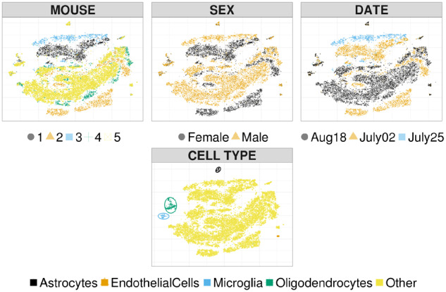
Unadjusted t-SNE coordinates. Points and shapes vary with batches

Figure 3 refers to adjusted t-SNE coordinates, estimated with Algorithm 1 using the same settings described in the simulation study. We compare BC-t-SNE with the same approaches used in the simulation studies. The first row of Figure 3 refers to BC-t-SNE; second and third to Harmony and MNN, respectively. Results suggest a satisfactory performance in terms of batch effect removal for all the methods considered. Indeed, BC-t-SNE embeddings from Figure 3 show no evidence of systematic variation with any of the batch variables under investigation. Such batches are marked by the colour and shape of points in Figure 3, showing that the batches are spread homogeneously across the embedded space after adjustment.

Fig. 3.

t-SNE coordinates after correction. Points and shapes vary with batches

Following the metrics used in the simulations, Table 3 quantitatively evaluates the success in removing batch effects. Results indicate that BC-t-SNE achieves a performance which is competitive with the other approaches. Focusing, for example, on mouse identifiers, the normalized silhouette coefficient suggests that BC-t-SNE removes batches more effectively than MNN and Harmony; similar conclusions hold also when kBET is considered. According to iLISI, instead, the baseline data adjustment methods perform better than BC-t-SNE. This result is not surprising, since such approaches optimize objective functions which are directly related to the iLISI metric (Korsunsky et al., 2019).

Table 3.

Evaluation of batch removal

		SIL	kBET	iLISI	pcR
BC-t-SNE	Sex	0.995	0.166	0.659	1.000
	Date	0.980	0.235	0.457	1.000
	Mouse	0.975	0.829	0.368	1.000
Harmony	Sex	0.997	0.299	0.846	1.000
	Date	0.987	0.421	0.540	1.000
	Mouse	0.975	0.854	0.498	0.999
MNN	Sex	0.999	0.219	0.844	1.000
	Date	0.996	0.392	0.546	1.000
	Mouse	0.958	0.794	0.502	0.999

Notes: Values range from 0 to 1, with higher values denoting more accurate removal of batch effects.

Lastly, it is important to investigate that after removing batch effects, clusters of cell types associated with medulloblastoma are preserved in the low-dimensional coordinates, and similar cells are close in the embedded space. Figure 4 shows results for BC-t-SNE and the baseline methods. The bulk of cells in a large central cluster is from tumours having markers within in a range of differentiation states, ranging from proliferative, undifferentiated cells expressing the SHH-pathway transcription factor Gli1, to cells in successive states of CGN differentiation, marked by sequential expression of markers Ccnd2, Barhl1, Cntn2, Rbfox3 and Grin2b (Ocasio et al., 2019). Clusters of cells surrounded with coloured ellipses correspond to endothelial cells, microglia, oligodendrocytes and astrocytes, which are common in the stroma within or adjacent to the tumours. Empirical findings suggest that such clusters are correctly preserved after adjustment; see also Table 4 for a quantitative evaluation.

Fig. 4.

t-SNE coordinates after adjustment. Points and shapes vary with cell types

Table 4.

Evaluation of cell-type preservation

	SIL	kBET	cLISI	pcR
BC-t-SNE	0.052	0.000	0.000	0.000
MNN	0.056	0.000	0.000	0.000
Harmony	0.031	0.000	0.000	0.000

Notes: Values range from 0 to 1, with lower values denoting more accurate preservation of cell-types.

5 Discussion

In this article, we have introduced BC-t-SNE, a novel modification of t-SNE, which allows for correction for multiple batch effects during estimation of the low-dimensional embeddings. The proposed approach has demonstrated good performance in simulation studies and on an application involving mouse medulloblastoma, where unwanted variations are successfully removed without removing information on differences across cell types.

A possible extension for future development involves adapting the proposed procedure to more efficient optimization of the t-SNE loss function, to overcome the computational constraints encountered with large n (Maaten, 2014). One way to address such an issue involves the use of alternative gradient methods, with methods based on stochastic gradients being popular in the literature.

Funding

The work of E.A. and D.B.D. was partially funded by the grant ‘Fair predictive modelling’ from the Laura & John Arnold Foundation, as well as grant 5R01ES027498 of the National Institute of Environmental Health Sciences of the United States Institutes of Health. We thank the UNC CGBID Histology Core supported by P30 DK 034987, the UNC Tissue Pathology Laboratory Core supported by NCI CA016086 and UNC UCRF and the UNC Neuroscience Center Confocal and Multiphoton Imaging and bioinformatics cores supported by The Eunice Kennedy Shriver National Institute of Child Health and Human Development [U54HD079124] and NINDS [P30NS045892]. D.L.F was supported by NICHD [F30HD10122801] and by NIGMS [5T32GM06755314]. J.O. was supported by NINDS [F31NS100489]. T.R.G. was supported by NINDS [R01NS088219, R01NS102627, R01NS106227] and by the UNC Department of Neurology Research Fund. T.R.G., K.W. and B.B. were supported by a TTSA grant from the NCTRACS Institute, which is supported by the National Center for Advancing Translational Sciences (NCATS), National Institutes of Health, through Grant Award Number UL1TR002489.

Conflict of Interest: none declared.

References

- Aliverti E. et al. (2018) Removing the influence of a group variable in high-dimensional predictive modelling. arXiv Preprint arXiv : 1810.08255. [DOI] [PMC free article] [PubMed]
- Butler A. et al. (2018) Integrating single-cell transcriptomic data across different conditions, technologies, and species. Nat. Biotechnol., 36, 411–420. [DOI] [PMC free article] [PubMed] [Google Scholar]
- Büttner M. et al. (2019) A test metric for assessing single-cell RNA-seq batch correction. Nat. Methods, 16, 43–49. [DOI] [PubMed] [Google Scholar]
- Cole M.B. et al. (2019) Performance assessment and selection of normalization procedures for single-cell RNA-seq. Cell Syst., 8, 315–328. [DOI] [PMC free article] [PubMed] [Google Scholar]
- Ellison D.W. et al. (2011) Medulloblastoma: clinicopathological correlates of SHH, WNT, and non-SHH/WNT molecular subgroups. Acta Neuropathol., 121, 381–396. [DOI] [PMC free article] [PubMed] [Google Scholar]
- Grün D., van Oudenaarden A. (2015) Design and analysis of single-cell sequencing experiments. Cell, 163, 799–810. [DOI] [PubMed] [Google Scholar]
- Haghverdi L. et al. (2018) Batch effects in single-cell RNA-sequencing data are corrected by matching mutual nearest neighbors. Nat. Biotechnol., 36, 421–427. [DOI] [PMC free article] [PubMed] [Google Scholar]
- Hastie T. et al. (2015) Statistical Learning with Sparsity: The Lasso and Generalizations. Chapman and Hall/CRC, Boca Raton, FL. [Google Scholar]
- Helms A.W. et al. (2000) Autoregulation and multiple enhancers control math1 expression in the developing nervous system. Development, 127, 1185–1196. [DOI] [PubMed] [Google Scholar]
- Hinton G.E., Roweis S.T. (2003) Stochastic neighbor embedding. In: Advances in Neural Information Processing Systems MIT Press, Cambridge, pp. 857–864.
- Hwang B. et al. (2018) Single-cell RNA sequencing technologies and bioinformatics pipelines. Exp. Mol. Med., 50, 96. [DOI] [PMC free article] [PubMed] [Google Scholar]
- Johnson W.E. et al. (2007) Adjusting batch effects in microarray expression data using empirical Bayes methods. Biostatistics, 8, 118–127. [DOI] [PubMed] [Google Scholar]
- Kobak D., Berens P. (2019) The art of using t-SNE for single-cell transcriptomics. Nat. Commun., 10, 1–14. [DOI] [PMC free article] [PubMed] [Google Scholar]
- Korsunsky I. et al. (2019) Fast, sensitive and accurate integration of single-cell data with harmony. Nat. Methods, 16, 1289–1296. [DOI] [PMC free article] [PubMed] [Google Scholar]
- Krijthe J.H. (2015) Rtsne: t-distributed stochastic neighbor embedding using barnes-hut implementation. R package version 0.15.
- Kruskal J.B. (1964) Multidimensional scaling by optimizing goodness of fit to a nonmetric hypothesis. Psychometrika, 29, 1–27. [Google Scholar]
- Lee J.A., Verleysen M. (2005) Nonlinear dimensionality reduction of data manifolds with essential loops. Neurocomputing, 67, 29–53. [Google Scholar]
- Leek J.T., Storey J.D. (2007) Capturing heterogeneity in gene expression studies by surrogate variable analysis. PLoS Genetics, 3, e161. [DOI] [PMC free article] [PubMed] [Google Scholar]
- Linderman G.C., Steinerberger S. (2019) Clustering with t-SNE, provably. SIAM J. Math. Data Sci., 1, 313–332. [DOI] [PMC free article] [PubMed] [Google Scholar]
- Luecken M.D., Theis F.J. (2019) Current best practices in single-cell RNA-seq analysis: a tutorial. Mol. Syst. Biol., 15, e8746. [DOI] [PMC free article] [PubMed] [Google Scholar]
- Lun A.T. et al. (2016) A step-by-step workflow for low-level analysis of single-cell rna-seq data with bioconductor. F1000Research, 5, 2122. [DOI] [PMC free article] [PubMed] [Google Scholar]
- Machold R., Fishell G. (2005) Math1 is expressed in temporally discrete pools of cerebellar rhombic-lip neural progenitors. Neuron, 48, 17–24. [DOI] [PubMed] [Google Scholar]
- Macosko E.Z. et al. (2015) Highly parallel genome-wide expression profiling of individual cells using nanoliter droplets. Cell, 161, 1202–1214. [DOI] [PMC free article] [PubMed] [Google Scholar]
- Mao J. et al. (2006) A novel somatic mouse model to survey tumorigenic potential applied to the hedgehog pathway. Cancer Res., 66, 10171–10178. [DOI] [PMC free article] [PubMed] [Google Scholar]
- McCarthy D.J. et al. (2017) Scater: pre-processing, quality control, normalization and visualization of single-cell RNA-seq data in R. Bioinformatics, 33, 1179–1186. [DOI] [PMC free article] [PubMed] [Google Scholar]
- McInnes L. et al. (2018) UMAP: uniform manifold approximation and projection for dimension reduction. arXiv Preprint arXiv : 1802.03426.
- Ocasio J. et al. (2019) SCRNA-seq in medulloblastoma shows cellular heterogeneity and lineage expansion support resistance to SHH inhibitor therapy. Nat. Commun., 10, 1–17. [DOI] [PMC free article] [PubMed] [Google Scholar]
- Risso D. et al. (2014) Normalization of RNA-seq data using factor analysis of control genes or samples. Nat. Biotechnol., 32, 896–902. [DOI] [PMC free article] [PubMed] [Google Scholar]
- Roweis S.T., Saul L.K. (2000) Nonlinear dimensionality reduction by locally linear embedding. Science, 290, 2323–2326. [DOI] [PubMed] [Google Scholar]
- Rubin L.L., de Sauvage F.J. (2006) Targeting the hedgehog pathway in cancer. Nat. Rev. Drug Discovery, 5, 1026–1033. [DOI] [PubMed] [Google Scholar]
- Tenenbaum J.B. et al. (2000) A global geometric framework for nonlinear dimensionality reduction. Science, 290, 2319–2323. [DOI] [PubMed] [Google Scholar]
- van der Maaten L. (2014) Accelerating t-SNE using tree-based algorithms. J. Mach. Learn. Res., 15, 3221–3245. [Google Scholar]
- van der Maaten L., Hinton G. (2008) Visualizing data using t-SNE. J. Mach. Learn. Res., 9, 2579–2605. [Google Scholar]
- Vieth B. et al. (2019) A systematic evaluation of single cell RNA-seq analysis pipelines. Nat. Commun., 10, 1–11. [DOI] [PMC free article] [PubMed] [Google Scholar]
- Vladoiu M.C. et al. (2019) Childhood cerebellar tumours mirror conserved fetal transcriptional programs. Nature, 572, 67–73. [DOI] [PMC free article] [PubMed] [Google Scholar]
- Wagner A. et al. (2016) Revealing the vectors of cellular identity with single-cell genomics. Nat. Biotechnol., 34, 1145–1160. [DOI] [PMC free article] [PubMed] [Google Scholar]
- Wolf F.A. et al. (2019) PAGA: graph abstraction reconciles clustering with trajectory inference through a topology preserving map of single cells. Genome Biol., 20, 59. [DOI] [PMC free article] [PubMed] [Google Scholar]
- Zappia L. et al. (2018) Exploring the single-cell RNA-seq analysis landscape with the SCRNA-tools database. PLoS Comput. Biol., 14, e1006245. [DOI] [PMC free article] [PubMed] [Google Scholar]
- Zurawel R.H. et al. (2000) Analysis of PTCH/SMO/SHH pathway genes in medulloblastoma. Genes Chromosomes Cancer, 27, 44–51. [DOI] [PubMed] [Google Scholar]