Having your cake and eating it too: Flexibility and power with mass univariate statistics for ERP data

Abstract

Event-related potential (ERP) studies produce large spatiotemporal datasets. These rich datasets are key to enabling us to understand cognitive and neural processes. However, they also present a massive multiple comparisons problem, potentially leading to a large number of studies with false positive effects (a high Type I error rate). Standard approaches to ERP statistical analysis, which average over time windows and regions of interest, do not always control for Type I error, and their inflexibility can lead to low power to detect true effects. Mass univariate approaches offer an alternative analytic method. However, they have thus far been viewed as appropriate primarily for exploratory statistical analysis and only applicable to simple designs. Here we present new simulation studies showing that permutation-based mass univariate tests can be employed with complex factorial designs. Most importantly, we show that mass univariate approaches provide slightly greater power than traditional spatiotemporal averaging approaches when strong a priori time windows and spatial regions are used. Moreover, their power decreases only modestly when more exploratory spatiotemporal parameters are used. We argue that mass univariate approaches are preferable to traditional spatiotemporal averaging analysis approaches for many ERP studies.

1. Introduction

In recent years it has become increasingly clear that many reported results in psychology and neuroscience are unreliable or do not replicate (e.g., Camerer et al., 2018; Open Science Collaboration, 2015; Pashler & Wagenmakers, 2012). This has generated a lot of discussion and reflection about methods, statistics, publication practices, and career incentives. As we will argue below, some of the key factors that lead to low replicability are magnified in EEG and ERP research. In particular, the large datasets generated in EEG research present opportunities for flexibility in analysis that is not sufficiently addressed by current practices in the field.

In this paper, we discuss issues in the analysis of ERP data that undermine our ability to draw strong conclusions and that contribute to spurious effects in the literature. We then propose that mass univariate analysis—an approach that has often been viewed as appropriate only for exploratory analysis in ERP research—offers an improvement over traditional spatiotemporal averaging approaches with regard to many of these issues. We present new software to implement mass univariate analyses for factorial designs, as well as simulation studies showing that these tests can provide greater power and greater flexibility than traditional analysis approaches while appropriately maintaining the Type I error rate.

1.1. Replicability as a function of both Type I error rate and power

There are many potential reasons for a failure to replicate findings. Assuming exact methodological replication (including sampling from the same population), the inability to replicate results is a problem of inferential error. It means that one of the studies (either the original or the replication) has reached the wrong conclusion. When such replication failures are common, it means that our procedures for making statistical inference are flawed, regularly producing either Type I errors (false positives: incorrectly concluding an effect exists) or Type II errors (false negatives: incorrectly concluding an effect does not exist). In fact, there are reasons to believe both kinds of errors are common.

A lot of discussion about replication failure has focused on “researcher degrees of freedom” (Simmons, Nelson, & Simonsohn, 2011) and their impact on the Type I error rate. Research in psychology and neuroscience often involves collecting multiple or multidimensional independent variables and dependent variables. Even for relatively simple designs, there are often many potential ways to process and analyze the data. When several effects are calculated in a study (due to multiple independent variables and/or dependent variables), or when data are analyzed in multiple different ways, this provides multiple chances to find an effect. Since each of these analyses has an independent (or partially independent) error rate, the probability that at least one test, or analysis path, will give a significant effect and appear to provide support for a hypothesis—even if there is no true effect—may be significantly higher than the nominal Type I error rate. In many cases, the multiple comparisons problem raised by complex designs and analysis flexibility is hidden or implicit, and it is therefore not always obvious that the probability of a false positive is greatly inflated (Cramer et al., 2016; Gelman & Loken, 2013; Kriegeskorte, Simmons, Bellgowan, & Baker, 2009; Luck & Gaspelin, 2017; Vul, Harris, Winkielman, & Pashler, 2009). As many authors have argued, this is a significant factor contributing to false positive effects in the literature (John, Loewenstein, & Prelec, 2012; Masicampo & Lalande, 2012; Simmons et al., 2011). As we will discuss below, this problem may be particularly prominent in ERP research.

A second factor contributing to low replicability is low power (or high Type II error rate). Of course, every researcher wants to have high power because we do not want to spend the time and resources it takes to conduct a study only to miss real effects. However, what is less often appreciated is that high power is also crucial for producing replicable effects—that is, power plays a role in our statistical inference, not just when we fail to find effects, but also when we observe significant results. This is for two reasons.

First, if we conduct a study with 50% power, we may well find a significant effect. However, if we attempt to replicate this result, it is equally likely that we will not be able to show the effect. What are we then to conclude? Which result should we trust? In the statistician R. A. Fisher’s (1966) words, “we may say that a phenomenon is experimentally demonstrable when we know how to conduct an experiment which will rarely fail to give us a statistically significant result” (p. 14). In the long run we draw important conclusions not from a single study, but from a number of studies. Unless we conduct research with consistently high power, the literature will always provide weak and/or contradictory evidence.

The second reason why power is important for producing replicable effects is that it influences the false discovery rate: the proportion of significant results that are false positives. A common misconception is that if we set α = .05, then only 5% of significant results will be false positives; that is, it is often mistakenly inferred that if a result is significant, there is a 5% chance that it is an error (Greenland et al., 2016; Haller & Krauss, 2002). However, α is the rate at which the null is rejected across all studies in which the null is true, and it therefore serves as an upper bound on the false positive rate across all studies conducted in the long-run. The proportion of false positives among the subset of studies that produce significant results is generally much higher. This proportion is called the false discovery rate, and it is a function of not only of the Type I error rate, but also of power.

To see the difference, imagine that we conduct 200 hypothesis tests. One hundred of these are cases in which the null is true and the Type I error rate is properly controlled at 5%; the other 100 are cases in which the alternative hypothesis is true (i.e., there is a true effect), but we only have 20% power to detect the effect. We would expect to find 25 significant effects: 5 in the cases where the null is true and 20 in the cases where the alternative is true. Thus, 20% of the significant effects are false positives, even though the Type I error rate is appropriately controlled at 5% (and only 2.5% of all studies conducted result in false positives). From this example, it should be obvious that if power is higher, the false discovery rate will be lower.

Especially when combined with publication bias (the tendency to only publish statistically significant results), a high false discovery rate can lead to a literature that is highly misleading and full of false positives. Thus, low power undermines our confidence that significant effects are real (for further discussion, see Button et al., 2013; Colquhoun, 2014). Unfortunately due to noisy measures and relatively expensive (in terms of both time and money) data collection, low powered studies are probably the norm in cognitive neuroscience (Button et al., 2013).

To summarize, a null hypothesis test only effectively discriminates between real effects and those due to sampling error when both Type I and Type II error rates are low. On the other hand, when both are high, it is actually possible that the majority of significant results obtained are false positives. This is the basis for John Ioannidis’s famous claim that “most published research findings are false” (Ioannidis, 2005).¹ It is therefore crucial that we address analysis flexibility and properly control the Type I error rate, but also that we do not do so at the expense of significantly reducing power.

1.2. Challenges of analyzing ERP data

EEG researchers (along with fMRI and MEG researchers) face additional statistical challenges beyond those faced by most behavioral researchers, because we collect thousands of measurements for each experimental condition. This is a necessary consequence of studying something as complex as neural activity. Moreover, as technology improves and new analysis approaches are developed, researchers are collecting even larger and more multidimensional datasets. However, flexibility in how we choose to analyze this large amount of data can significantly increase the Type I error rate.

Consider a simple ERP experiment in which measurements are recorded from 32 electrodes at a sampling rate of 500 Hz. Epochs extending to 1000 ms after stimulus onset are extracted from this data. Even after individual trials are averaged, there are 16,000 data points for each subject in each experimental condition. This presents a massive multiple comparisons problem. That is, in such an experiment, it is almost guaranteed that in some time window at some point on the scalp there will be an effect that reaches significance in a conventional analysis, even if the null hypothesis is true at all time points and electrodes. It follows that the presence of an effect that reaches statistical significance is only evidence that a true effect exists if the multiple comparisons issue is appropriately addressed. Unfortunately, the most common ways of analyzing ERP data do not sufficiently address this problem. This issue has been reviewed in detail by Luck and Gaspelin (2017), so we will only briefly describe it here (see also, Kilner, 2013; Kriegeskorte et al., 2009; Luck, 2014, Chapter 10).

1.2.1. Traditional approaches to ERP analysis: Spatiotemporal averaging

The most common way to handle the large amount of data collected in an ERP study is to reduce it via spatiotemporal averaging prior to statistical analysis. In the time domain, an effect can be measured by calculating the maximum or minimum value (peak amplitude) or the average value (mean amplitude) across a particular time window (Luck, 2014, Chapters 9–10). In the spatial domain, data can be reduced by choosing a representative electrode or by averaging across a subset of electrodes that are selected to reflect the typical spatial distribution of the effect of interest. For example, an ERP researcher may operationalize the N400 component as the mean amplitude from 300 to 500 ms, averaged across a spatial region of centroparietal electrodes (e.g., Cz, CP1, CPz, CP2, Pz). With this approach, the Type 1 error rate can be controlled by eliminating researcher degrees of freedom altogether: that is, by fully specifying a priori the spatial region and the time widow of interest. Particularly if these procedures are preregistered (Chambers, Feredoes, Muthukumaraswamy, & Etchells, 2014; Lindsay, Simons, & Lilienfeld, 2016; Nosek, Ebersole, DeHaven, & Mellor, 2018), we can then be confident that reported p-values are accurate and that error rates of the tests are appropriately controlled (given, of course, that other assumptions of the test hold).

The problem with this approach is that it is overly rigid and can potentially dramatically reduce power to detect effects: if a time window and spatial region are chosen a priori, and they do not coincide with the effect of interest, an experimenter will be unable to detect a true effect. Importantly, this situation is the norm: many ERP effects are variable in timing and/or scalp distribution, and so it is not always obvious how to choose the time window(s) and spatial region before data is collected. For example, despite its name, the classic P300 component is defined more by its morphology, posterior scalp distribution, and sensitivity to particular experimental manipulations, than by its precise timing. Indeed, P300 effects can vary by several hundred ms due to factors that may be of little theoretical interest for a given study (Kutas, McCarthy, & Donchin, 1977). Other components, such as the N400, may have stable timing (Federmeier & Laszlo, 2009), but they can vary in scalp distribution depending on the precise nature of the stimuli (Holcomb, Kounios, Anderson, & West, 1999; Kutas & Federmeier, 2011). Moreover, even if identical stimuli are used, there may be differences between studies in the precise scalp distribution of an effect because of differences between individuals and populations, both in the precise neuroanatomical sources activated, and in structural and functional neuroanatomy, leading to different projections of these sources on to the scalp surface. Thus, even if a researcher has a well-motivated, clear, a priori hypothesis about a well-studied component and how its amplitude will be modulated, she may not know in advance the exact time window or spatial ROI that will best characterize this component. For studies in which the researcher has little or no a priori prediction about where and/or when an effect will manifest, the mean amplitude approach may be so restrictive as to make useful analysis impossible.

Many researchers recognize this issue and have adopted two main methods of increasing flexibility while still using spatiotemporally averaged ERP data as the dependent variable. Unfortunately, however, as we discuss next, both of these practices reintroduce the problems of Type 1 error.

The first way that some researchers increase flexibility in analysis is to select analysis parameters based on visualization of the data. This remains fairly common practice, but, as discussed extensively by Luck and Gaspelin (2017), it introduces significant bias. Choosing a time window and/or spatial ROI based on where differences are observed in the data is essentially equivalent to conducting an analysis in many different time windows and regions and reporting the one that produces the largest effect. Framed in this way, the multiple comparisons problem and inflation of the Type I error rate should be obvious. Because all these many possible analyses are not actually conducted, this is often called the problem of implicit multiple comparisons (Luck & Gaspelin, 2017; see also Gelman & Loken, 2013), and many researchers appear unaware of the extent to which this can inflate the Type 1 error rate and undermine confidence in significant results.

The second way in which researchers have attempted to increase flexibility in analysis is more principled in nature: either spatial regions and/or temporal window are included as additional factors in the statistical model. For example, electrodes may be divided up into different spatial regions and entered into a repeated measures ANOVA with a hemisphere factor and an anterior-posterior factor. It is then possible to examine main effects of the experimental condition(s) of interest and the interaction of these effects with spatial factors. This approach has the advantage of eliminating the need to choose a spatial region a priori. As we discuss next, however, this approach introduces a new multiple comparisons problem.

To understand how to interpret an interaction with a spatial factor in this type of ANOVA, it is important to understand the biophysical basis of EEG/ERP (for a more detailed explanation see Buzsáki, Anastassiou, & Koch, 2012; Luck, 2014). The postsynaptic potentials that generate ERPs create electrical dipoles: that is, they generate a positive voltage on one side of a particular region of cortex and a corresponding negative voltage on the other side. The electrode montage on the scalp only covers approximately half of a full sphere. Thus, if a dipole is oriented vertically, only one side will be recorded and all or most of the electrodes on the scalp will record voltage in the same direction. If the dipole is oriented horizontally, both sides will be recorded, and a component will appear as a positive deflection at some sites and a negative deflection at others. In either case, each neural source will project with different weights to different electrodes. Thus, all effects (both those composed of a single dipole and those composed of multiple additive dipoles) should yield an interaction between experimental condition and electrode/region. Moreover, since the positive and negative ends of a dipole will never cancel each other perfectly across the recorded electrodes, all effects will also generate a main effect. Whether the main effect and/or the interaction effect is detected (reaches statistical significance) is simply a combination of dipole orientation and strength (for further discussion of the interpretation of such interactions, see Luck, 2014; McCarthy & Wood, 1985; Urbach & Kutas, 2002, 2006). Thus, the inclusion of a spatial factor in an ANOVA model gives every effect two independent chances of reaching significance.² If multiple spatial factors are included, the problem increases exponentially (e.g., with two spatial factors, every effect has four chances to reach significance). This leads to a significant inflation of the Type I error rate.³

Although not quite as common, some researchers attempt to increase the flexibility of analyses in the temporal domain by measuring multiple time windows and including time window as a factor in a single repeated measures ANOVA. This raises similar multiple comparisons concerns. In addition, this approach is likely to have low power when effects exist in only one or a few of many time windows tested.

To sum up, we face a catch-22 in analyzing ERP data. To consistently have high power to detect effects across space and time, we require flexibility in our analysis approaches. Yet the most common approaches in ERP research do not allow for much flexibility without increasing the Type I error rate. As a result, there is very much a “damned if you do, damned if you don’t” aspect to choosing time windows and spatial regions in ERP analysis. While several methods have been proposed to deal with this dilemma within the traditional spatiotemporal averaging approach (Brooks, Zoumpoulaki, & Bowman, 2017; Luck & Gaspelin, 2017), none is wholly satisfactory for all situations.

1.3. Mass univariate statistics for ERP data

An alternative method of dealing with the implicit multiple comparisons problem in ERP data is to make it explicit. Rather than average across time and space, we can calculate a separate statistical test at multiple time points and electrodes individually. We then apply a multiple comparisons correction to control the family-wise Type I error rate across these many independent tests. Because this method deals with a large number of dependent variables by conducting many univariate analyses, it is referred to as a “mass univariate approach”.

The key to making the mass univariate approach practical is to employ a multiple comparisons correction that provides adequate power. Therefore, specialized corrections are generally used. In EEG research, two main classes of corrections are common. The first makes use of probability theory to control the false discovery rate (FDR) within a family of comparisons (i.e., across electrodes and time points). Various formulas for the false discovery rate correction have been proposed based on differing assumptions. We explore three in the present work: the Benjamini and Hochberg (1995) procedure, which assumes the results of the family of tests are independent or positively correlated; the Benjamini, Krieger, and Yekutieli (2006) procedure, which also assumes independent or positively correlated tests but is intended to offer better power when a low proportion of true effects exists across tests; and the Benjamini and Yekutieli (2001) procedure which controls the false discovery rate regardless of the correlation between tests.

The second class of mass univariate corrections use resampling procedures to estimate the null distribution of specialized statistics to control the familywise error rate. These methods are nonparametric in nature and therefore require fewer assumptions about the distribution of the data than parametric tests (FDR corrections can also be used with nonparametric tests, but they are generally used with parametric analyses). Two approaches have received the most attention in EEG research. The first uses a permutation approach to estimate the null distribution of the maximal effect (e.g., the largest t- or F-value) across time points and electrodes (t_max or F_max; Blair & Karniski, 1993). The second uses a permutation approach to estimate the null distribution for a cluster statistic (i.e., a statistic representing the size of a cluster of adjacent time points and electrodes showing an effect larger than some prespecified threshold; Bullmore et al., 1999; Maris & Oostenveld, 2007). An alternative resampling approach to these permutation-based methods is to use bootstrapping to estimate the null distribution of the same or similar statistics (e.g., Pernet, Chauveau, Gaspar, & Rousselet, 2011; Pernet, Latinus, Nichols, & Rousselet, 2015; see further discussion in the Supplementary Materials). In the present study, we focus on the two permutation-based approaches that have been most commonly used to date, but we review the various mass univariate corrections in more detail in the Supplementary Materials (see also Groppe, Urbach, & Kutas, 2011a; Luck, 2014, Ch. 13; Pernet et al., 2011; Pernet et al., 2015).

Mass univariate approaches are certainly not new or novel for cognitive neuroscientists. In fact, they are at the core of standard analysis approaches in functional MRI research (Woolrich, Beckmann, Nichols, & Smith, 2009). They are also commonly used for analysis of EEG in the frequency domain. However, for standard cognitive ERP research, mass univariate analysis is currently used much less commonly than the traditional spatiotemporal averaging approaches described above.

One likely reason for this is historical. The standards and common practices for ERP analyses were developed when arrays of only a few electrodes were common, when computing power made complex, multidimensional analysis approaches difficult or impossible, and before many of the specialized multiple comparison corrections in use today had been developed. As a result, ERP researchers became accustomed to measurement approaches that reduce the large amount of data prior to statistical analysis (which, as discussed above, also makes the multiple comparisons issue much less obvious). In contrast, early fMRI research was often searching for where effects would appear across many voxels, which made the multiple comparison problem explicit. In addition, standard fMRI analysis approaches were developed after important advances in computing power and multiple comparisons corrections for large datasets had been devised. The result was that very different practices became standard, despite the common statistical challenges faced in analyzing fMRI and ERP data.

However, there are additional reasons, beyond tradition and inertia, for why mass univariate approaches have not become common in ERP research. We can identify two key barriers to their widespread adoption.

This first is that current widely used software implementing mass univariate approaches for ERP data (Mass Univariate Toolbox: Groppe et al., 2011a; FieldTrip: Oostenveld, Fries, Maris, & Schoffelen, 2011) only support single factor designs, or designs that can be reduced to a single factor (however, for a bootstrap-based approach to mass univariate analysis with complex designs, see the LIMO MEEG toolbox: Pernet et al., 2011). The reason for this is that the permutation-based corrections that have been most popular in ERP research are not straightforward for factorial designs. As explained in detail in the Supplementary Materials (section 1.2), the problem for permutation-based factorial ANOVA designs is determining which observations are exchangeable (and thus permutable) under the null hypothesis for a particular effect, in cases when it cannot be assumed that the null is also true for other effects in the design. The upshot is that for some effects in factorial designs (particularly interaction effects), it is only possible to construct an approximate test that controls the Type I error rate asymptotically as the sample size increases (Anderson, 2001; Anderson & Ter Braak, 2003). Since researchers are often interested in interaction effects in factorial designs, mass univariate statistics are only likely to see widespread use if they are able to handle these effects.

The second, and perhaps more important, reason why mass univariate approaches have not yet been widely adopted in ERP research is that they are often perceived as being primarily suited for exploratory analysis. Many researchers we have talked to assume that mass univariate approaches sacrifice power for flexibility and that they should be reserved for situations where researchers have little idea about the spatial and temporal characteristics of the effects of interest. Indeed, existing work on mass univariate approaches has generally discussed them primarily in this context (e.g., Groppe et al., 2011a; Lage-Castellanos, Martinez-Montes, Hernandez-Cabrera, & Galan, 2010; Luck & Gaspelin, 2017). This is understandable: multiple comparison corrections generally reduce power and, in most cases, the larger the multiple comparisons problem, the larger the reduction in power. However, as we discuss next, the power of mass univariate approaches, in comparison with traditional mean amplitude approaches, has not yet been systematically explored.

1.4. The present work: Simulations of the type I error rate and the power of mass univariate approaches

The goal of the remainder of this paper is to directly address these two barriers to the use of mass univariate statistics in ERP research, and, more generally, to address the challenge of how best to balance the need for flexibility, power, and Type I error control in ERP analysis.

To address the first barrier, the first author has developed and released the Factorial Mass Univariate Toolbox (FMUT; Fields, 2017b), which builds upon and extends the existing Mass Univariate Toolbox developed by David Groppe (Groppe et al., 2011a).⁴ This free and open source MATLAB toolbox implements mass univariate approaches for factorial ANOVA, which extends that ability to conduct mass univariate statistics to a much broader range of experimental designs used in ERP research.⁵ Here we use FMUT to conduct a series of simulation studies to explicitly address issues of Type 1 error (for permutation-based approaches) and power. We address two key questions.

First, we evaluate the Type 1 error rate for permutation-based mass univariate approaches with factorial designs. Specifically, we ask whether the approximate permutation-based methods that are necessary with some factorial ANOVA designs can appropriately control Type I error rate with realistic ERP data and the multiple comparisons corrections commonly used in mass univariate statistics. There are various methods for constructing an approximate test in these situations. Previous simulation work in other domains has suggested that calculating and permuting residuals (see the Supplementary Materials for a description of this approach) is generally the preferred method, as it controls the Type I error rate well even in small samples (Anderson & Ter Braak, 2003; Still & White, 1981; Winkler, Ridgway, Webster, Smith, & Nichols, 2014). However, it is important to determine whether these results extend to ERP data so that researchers can be confident when applying permutation-based mass univariate statistics to the wide range of experimental designs used in ERP research (i.e., designs with more than one factor).

Second, using realistic EEG noise and ERP effects, we ask how the power of mass univariate approaches compares to traditional mean amplitude analyses. Here, we consider both permutation-based approaches (F_max and cluster-based corrections) as well as the three different FDR corrections described above. Importantly, instead of simply comparing the traditional approach to fully exploratory mass univariate approaches, we examine the relative power of each approach under varying degrees of specificity about the time windows and spatial regions that correspond to an effect of interest. This allows us to directly contrast the power of the mean amplitude approach and various mass univariate approaches when strong a priori assumptions about the timing and scalp location of a particular ERP effect are available, and to examine the relative power of these approaches as these assumptions are relaxed.

2. Method

Simulation studies were conducted via custom MATLAB code. All code is available on the Open Science Framework (OSF) page for this project: https://osf.io/mktqj/.

2.1. Extraction of EEG noise data

Following Groppe, Urbach, and Kutas (2011b), we carried out all our simulation studies using trial-level noise from real EEG data. To obtain EEG noise, we used preexisting EEG data collected in our lab from 49 subjects who completed the AX-CPT task (a measure of cognitive control processes: Servan-Schreiber, Cohen, & Steingard, 1996).⁶ In this task, participants see a series of letters and press a button whenever they see the letter X preceded by the letter A. We used this dataset simply because it contained a relatively large number of subjects and a large number of trials for each subject. This allowed us to simulate studies by randomly sampling from subjects and trials, as detailed below.

Briefly, EEG data was recorded from 32 Ag/AgCl electrodes using a BioSemi ActiveTwo system (biosemi.com), low-pass filtered online at 102.4 Hz, and continuously sampled at 512 Hz. In EEGLAB (sccn.ucsd.edu/eeglab; Delorme & Makeig, 2004) and ERPLAB (erpinfo.org/erplab; Lopez-Calderon & Luck, 2014), the continuous EEG was referenced offline to the average of the mastoids and high-pass filtered at 0.05 Hz. Then epochs were extracted from 200 ms before until 1100 ms after each letter, and baseline corrected by subtracting the mean voltage from −200 to 0 ms of each epoch. Trials with artifact (blinks, eye movements, bad channels, etc.) were detected using algorithms implemented in ERPLAB and discarded. This left an average of 659 trials for each of the 49 subjects (range: 516 to 771). The remaining trials were low-pass filtered at 30 Hz and downsampled to 128 Hz.

We used these trials to extract epochs of background EEG noise as follows. In each participant, for each epoch, at each of the 32 electrode sites, the averaged waveform (i.e., the ERP) of that trial’s experimental condition was subtracted from the raw EEG. For example, for the AX condition, the average waveform for all AX trials was subtracted. This removed (an estimate of) the event-related activity and left the individual trial-level EEG background noise. These noise trials sum and average to zero across all trials within and across conditions and participants (i.e., no overall effects of condition or subject remain), thus reflecting the null hypothesis.

The advantage of using actual EEG data in this way is that it represents realistic variability across electrodes, time points, trials, and subjects. The full complexity of this variability would be difficult to simulate due to the large variety of sources of variability in an EEG study. These include stable individual differences in cognition and anatomy, differences in cognitive state due to time of day or sleepiness, differences in equipment set-up across participants (e.g., cap positioning), fatigue effects across the study, differences in the structure of the variability of the waveform in early and late time windows, and many other factors. Having realistic variability is important, both because it affects the power of various mass univariate approaches, and because some approaches, like the Benjamini and Hochberg (1995) and Benjamini et al. (2006) FDR corrections, rely on assumptions about the correlation between different time points and electrodes. Thus, the effects of violations of these assumptions are reflected in our simulation results.

2.2. Simulations of the Type I error rate of approximate permutation tests required for factorial ANOVA designs

As noted in the Introduction and discussed in detail in Supplementary Materials, by calculating and permuting residuals, it is possible to construct approximate permutation tests for factorial designs that control Type I error rate asymptotically as the sample size increases (for details, see Supplementary Materials and Anderson & Ter Braak, 2003; Still & White, 1981; Winkler et al., 2014). Our first aim was to use these methods to simulate the Type 1 error rate for an interaction effect in a 3 × 3 repeated measures ANOVA. We examined a 3 × 3 interaction because this is the simplest effect for which an approximate permutation test is required. We used two permutation-based mass univariate corrections to account for multiple comparisons: the F_max and cluster mass procedures. Our question was whether these methods maintain the Type I error rate at an acceptable level with realistic EEG data.

For each test, we simulated 10,000 experiments. To simulate each experiment, we drew upon a random subset of participants and a random subset of their noise trials (calculated as described above). We varied the number of participants (40, 25, 16, 12, and 8) and the number of trials (40, 20, and 10 per condition) to examine the effects of these parameters on the Type I error rate. Within each subject, we randomly assigned the noise trials (i.e., the entire electrode x time point matrix from each trial) to each of nine arbitrary conditions. This created a situation in which the distribution and structure of variability in the EEG signal across subjects, time points, and electrodes was realistic, but there was no true difference in the ERP across the nine conditions. That is, the null hypothesis was known to be true in the population that subjects and trials were sampled from, but nonzero differences would be expected to emerge by chance through random sampling in a way consistent with actual ERP experiments. The relevant question was how often this random sampling error would lead to significant effects.

For each simulated experiment, we carried out a 3 × 3 permutation ANOVA, testing the interaction effect via the permutation of residuals method at each of the 32 electrode sites at each sampling point. Because variability is likely to differ in early and later portions of the ERP (e.g., slow drift will affect later time points more than earlier time points), we separately examined an early time window of 0–300 ms and a later time window of 300–1000 ms.

We first simulated the Type 1 error rate with the F_max correction for multiple comparisons. For each simulated experiment, we conducted 5,000 random permutations⁷ of the data and identified the maximum F-value across all time points and electrodes for each permutation. These 5,000 “F_max” values formed the null distribution, and any time point and electrode with an F-value in the unpermuted data that was greater than 95% of values in this null distribution was considered significant. We calculated the Type I error rate as the percentage of the 10,000 simulated studies where at least one time point/electrode reached significance.

We then simulated the Type 1 error rate using the cluster mass correction for multiple comparisons. Clusters were defined as adjacent time points and/or electrodes with F-values that would be statistically significant at one of two alpha levels (see below). For the purposes of clustering, electrodes within approximately 7.5 cm of one another (assuming a head diameter of 56cm) were considered adjacent; adjacent time points were any consecutive samples. The cluster statistic was defined as the sum of all F-values in a cluster and the null distribution for this statistic was estimated by identifying the largest cluster across each of 5,000 random permutations of the data for each simulated experiment. Any cluster in the original, unpermuted data larger than 95% of clusters in the null distribution was considered significant. We calculated the Type I error rate as the percentage of all simulated studies that revealed at least one significant cluster.

2.3. Simulations of power for realistic ERP effects

Our second aim was to simulate studies in order to examine the power of different mass univariate approaches: two different permutation-based approaches—the F_max test and the cluster mass test—and three different versions of the false discovery rate (FDR) correction. We compared each of these mass univariate methods to the traditional mean amplitude analysis approach, as well as to each other, with varying a priori assumptions about spatiotemporal location.

2.3.1. Construction of simulated experiments

Experiments were simulated according to the procedures described above for tests of the Type I error rate with the following differences: (1) the number of simulated conditions differed depending on the effect being tested; (2) as our goal was to compare the relative power of different methods rather than power curves or absolute power, 24 subjects and 20 trials per condition were used for all simulations to simplify simulations and results; (3) realistic ERP effects were added to the data after the noise was randomly sampled and averaged.

In order to simulate individual differences in effects, in each simulated experiment, we multiplied the entire electrode x time point matrix of the effect of interest (see below) by a value randomly drawn from a normal distribution with a mean of 1 and a standard deviation of 0.1 for each condition for each subject. Then, for each effect in each simulated experiment, we added the averaged noise trials so that the simulated waveforms represented the sum of a true population level effect (with individual differences) and realistic EEG noise.

2.3.2. Simulated effects

We examined three ERP effects: the N400, the P300, and a simulated early, focal P1. The first two were chosen because they are widely studied, well-known ERP components that many researchers will be familiar with. The P1 was included to examine power to detect a spatially and temporally focal effect. These three effects are shown in Figure 1. The data for these effects is available on the OSF page for this project: https://osf.io/mktqj/.

Figure 1. Real ERP effects used in simulations of power.

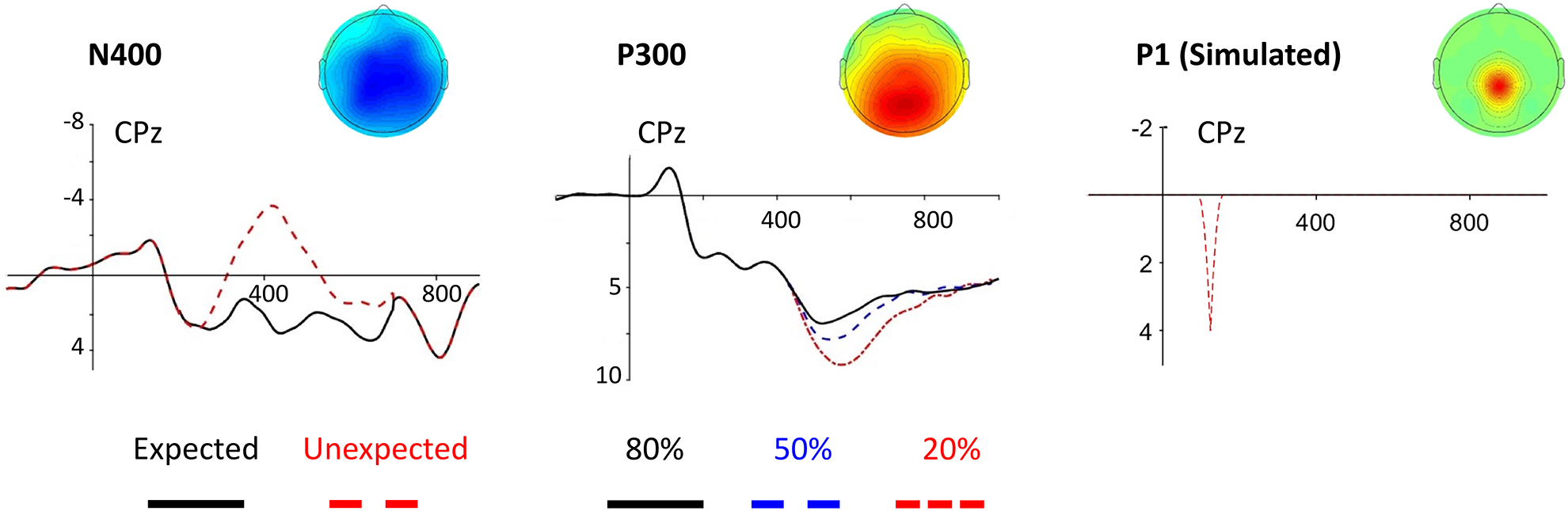
See text for details.

To simulate the well-established effect of semantic expectancy on the N400, we used the 7.5 Hz low-pass filtered grand average waveform of two conditions from a subset of subjects (n = 24) who took part in an experiment carried out by Kuperberg, Brothers, and Wlotko (2019): highly expected critical words (high cloze probability) in a highly constraining sentence context and unexpected (low cloze, but plausible) critical words in a nonconstraining context. The effect was centroparietally distributed and peaked at around 430 ms. For the purposes of the simulation, all time points before 200 ms and after 700 ms at all electrodes were set to the average of the two conditions (i.e., the null hypothesis was true). Because the N400 effect size in this study was quite large, power would approach or equal 1 for some of the analyses presented here. We therefore reduced the size of the effect, relative to the error trials, by a third (i.e., the effect represented what may be expected from a similar, but subtler, semantic manipulation).

To simulate the P300, we used the 7.5 Hz low pass filtered grand average waveform of the 20%, 50%, and 80% conditions of a traditional two-stimulus oddball task with male and female names as the stimulus categories (Fields, 2017a, Chapter 2). As shown in Figure 1, this effect peaked at around 620 ms and was centroparietally distributed (replicating Fabiani, Karis, & Donchin, 1986). All time points before 430 ms and after 980 ms at all electrodes were set to the average of the two conditions (i.e., the null hypothesis was true). Because this effect was quite large, the size of the effect relative to the error trials was reduced by half to avoid ceiling effects.

Previous simulation work by Groppe et al. (2011b) indicates that the relative power of the different mass univariate approaches depends on the nature of the effect being tested. The N400 and P300 are both widely distributed in space and time, and they are generally rather similar in their spatiotemporal characteristics. We did not have access to a more focal effect that matched our noise data (i.e. that was collected with the same electrode array and equipment), so we simulated a focal P1-like effect. This effect consisted of a quadratic parabola lasting 7 sampling points (approximately 50 ms given a 128Hz sampling rate) and representing a 4 μV difference at the peak. The effect was added starting at 98 ms at CPz and a half-amplitude version of the effect was added to the four electrodes surrounding CPz: Cz, CP1, CP2, and Pz (this made the spatial distribution similar to the other effects examined here). In other words, this effect was short-lived, peaked sharply, and was very focal on the scalp (see Figure 1).

2.3.3. Calculation of statistical tests

To examine the power of the traditional averaged amplitude approach, the mean amplitude across all time points and electrodes included in the analysis (see below) was submitted to a parametric repeated measures ANOVA for each simulated experiment. Power was defined as the proportion of the 10,000 simulated experiments where the effect reached a significance threshold of p ≤ .05.

To examine the power of each mass univariate approach, a separate repeated measures ANOVA was conducted at each electrode and time point included in the analysis, and the relevant correction was applied. The permutation-based corrections were calculated as described above. We examined the cluster mass approach with two cluster inclusion thresholds, an uncorrected p-value of .05 and an uncorrected p-value of .01. While p ≤ .05 has been used in most work, we suspected that the more stringent inclusion criteria would magnify the influence of large effect sizes at the peak, which may make the cluster approach more sensitive to focal effects like the simulated P1. Finally, we calculated three FDR corrections as described by Benjamini and Hochberg (1995), Benjamini and Yekutieli (2001), and Benjamini et al. (2006), respectively. For each of these approaches, we calculated power as the percentage of 10,000 simulated experiments where any time point/electrode combination (or in the case of the cluster mass test, any cluster) was significant at a corrected level of p ≤ .05.

2.3.4. Assessing power of different approaches to detect effects under varying a priori assumptions about spatiotemporal location

Our key question was about familywise power: the proportion of all simulated studies in which at least one time point was (correctly) identified as significant. In other words, assuming an effect is present, how likely is each method to detect it?

We first examined familywise power in a priori time windows and spatial ROIs that matched well where we knew the effect was actually located. These simulations represented the approach generally taken when using mean amplitude analyses. We then progressively relaxed these temporal and spatial assumptions to examine the effect of increased analysis flexibility on the power of each approach. This allowed us to ask two key questions. First, how does the power of traditional approaches compare to mass univariate approaches when the temporal and spatial distribution of the effect is known a priori? Second, how much power is lost when these assumptions are relaxed to reflect uncertainty about the timing or location of effects? This is in contrast to previous simulation work that has examined the power of the mass univariate approach for less realistic ERP effects and only as a purely exploratory approach (Groppe et al., 2011b; Lage-Castellanos et al., 2010).

2.3.5. Using mass univariate approaches to detect the time course of effects

Standard spatiotemporal averaging analysis approaches in ERP research are intended to answer the question of whether a difference between conditions exists at all, and they are generally ill-suited to tell us precisely when and where an effect exists. That is, if we analyze the N400 as the mean amplitude from 300–500 ms, and we find a significant effect, this does not tell us that the effect exists at all time points between 300–500 ms, nor does it tell us whether or not the effect extends beyond this prespecified time window. Our main goal in the analysis of the power of mass univariate tests, as described above, was to determine their power to answer this same question: whether there is any significant difference in a given time window. Thus, power was defined as the percentage of studies in which any time point reached significance (familywise power).

Unlike the mean amplitude approach, mass univariate approaches also give us some explicit information about the temporal extent of an effect because we can see which individual time points reach significance in a mass univariate analysis. Even though most mass univariate methods are not guaranteed to be accurate for individual time points (see Discussion), we examined how well each of these approaches characterizes the timecourse of effects by calculating the following three measures from our simulations:

• Elementwise power: For each study that shows at least one significant time point, what proportion of time points with a true effect are significant? In other words, if one finds a significant effect using a given correction, to what extent is the time course revealed by that correction likely to capture the full extent of the true effect?

• Familywise false discovery rate (FDR): Out of all studies that show at least one significant time point, what proportion of these studies include at least one false positive? In other words, if one finds a significant effect using a given correction, what is the likelihood that some of the time points revealed are actually false positives?

• Elementwise false discovery rate (FDR): For each study that shows at least one significant time point, what proportion of time points that are significant are actually false positives? In other words, if one finds a significant effect using a given correction, do most of the time points revealed reflect true effects, or is there likely to be a large proportion of false positives?

Additional measures, including elementwise Type I error rate, onset times, and offset times, are available on the OSF page for this project: https://osf.io/mktqj/

3. Results

Full results of all simulations are available on the OSF page for this project: https://osf.io/mktqj/.

3.1. Simulations of the Type I error rate of approximate permutation tests

Our first aim was to simulate the Type 1 error rate for the two-way interaction effect in a 3 × 3 repeated measures ANOVA using approximate permutation-based tests (see Introduction and Supplementary Materials) with the F_max and cluster mass corrections. For each simulated experiment we calculated the Type I error rate as the percentage of simulated experiments in which any time point/electrode reached significance at p ≤ .05.

Results are shown in Figure 2. As can be seen, the permutation of residuals method of constructing the approximate permutation test led to only a minimally inflated Type I error rate. Cluster-based methods maintained the Type I error rate better than the F_max method in all simulations. As expected, the Type I error rate was increased with smaller sample sizes. However, even for simulations with only 8 subjects and 10 trials per condition—both of which are rather extreme for most ERP studies—the Type I error rate was only .077 for the F_max methods and .068 for the cluster mass test. For most simulations, rates were much closer to the nominal α.

Figure 2. Type I error rate of approximate permutation tests.

Bar graphs show the Type I error rate of the permutation of residuals method for a 3 × 3 ANOVA interaction with varying numbers of subjects and trials. Type I error rate for mean amplitude (averaged across time points and electrodes) with parametric ANOVA is shown for reference. Error bars show the Clopper-Pearson 95% confidence interval of the proportion.

3.2. Simulations of power to detect realistic ERP effects

Our second aim was to examine the relative power of the different mass univariate correction approaches: permutation approaches with the F_max and the cluster mass corrections (with two different cluster inclusion thresholds), and three versions of the false discovery rate correction. We compared all these mass univariate methods with the traditional mean amplitude analysis approach with regard to ability to detect effects on three different ERP components: the semantic expectancy effect on the N400 component, the oddball effect on the P300, and a simulated temporally and spatially focal P1-like effect. Importantly, we examined the power of each of these methods to detect effects both under the assumption that the experimenter had strong a priori knowledge about spatial location and time window (strong spatiotemporal regions of interest), and with more exploratory analysis parameters.

3.2.1. N400

3.2.1.1. Power to detect N400 modulation under different a priori assumptions about its spatiotemporal location

We first examined the N400 effect within a constrained a priori spatiotemporal region of interest that is typically associated with the N400 component and that corresponded to where the effect was actually observed in the studies that we simulated: a time window of 300–500 ms and a spatial region of five centroparietal electrodes (Cz, CP1, CPz, CP2, Pz). As shown in Figure 3, the F_max and cluster mass tests showed slightly better power than the mean amplitude approach. The false discovery rate based tests had the least power of all the approaches, particularly the more conservative Benjamini and Yekutieli (2001) method.

Figure 3. Familywise power.

Plotted is the proportion of all simulated studies where at least one time point was correctly identified as showing an effect. Error bars show the Clopper-Pearson 95% confidence interval of the proportion.

We next carried out simulations with a less restrictive spatiotemporal region of interest: all electrode sites within a time window of 200–600ms. As would be expected, averaging across this broader spatial and temporal region greatly reduced the power of the mean amplitude approach. In contrast, the cluster mass approach displayed approximately the same power as in the more restrictive analysis. The other mass univariate approaches showed moderately reduced power, but all of them (with the exception of the Benjamini and Yekutieli (2001) FDR correction) showed much greater power than the mean amplitude approach. Finally, we carried out a completely bottom-up, exploratory approach examining the entire temporal epoch at all electrode sites. In this simulation, the mass univariate approaches—especially the cluster mass test—showed only moderately reduced power.

3.2.1.2. Using mass univariate approaches to detect the time course of the N400

Above we considered the power of mass univariate methods to detect whether any effect was present within a prespecified time window. As noted in the Methods, this is the question answered by the spatiotemporal averaging approache to analysis.

Unlike these traditional methods, mass univariate analyses also allow us to examine the rejection rates at each individual time point, allowing us to determine how well each correction method accurately characterizes the timecourse of our simulated effects. To address this question, we focus on the 0–1000 ms analysis at all electrode sites. This is because the analyses carried out between 300–500 ms and 200–600 ms analyses contained only time points with true effects, and so false positive time points were not possible in these analyses (full results for all analyses are available at https://osf.io/mktqj/).

3.2.1.2.1. Elementwise power:

As shown in Figure 4, all mass univariate methods tended to underestimate the true duration of the effect, generally reporting less than half of time points that had a true effect across the full epoch. The .05 thresholded cluster mass test generally showed the best performance in this regard. The F_max and Benjamini and Yekutieli (2001) FDR approaches showed the worst performance, particularly underestimating the duration of the true effects.

Figure 4. Elementwise power.

Elementwise power is defined as the proportion of time points with a true effect that were indicated as significant. Plots show the distribution of this proportion across the subset of all simulated studies where at least one time point was significant. The black bar shows the median, the limits of the box show the 25^th and 75^th percentile, and the lines extend to the 5^th and 95^th percentile. (Note that the box is missing in some places because the median, 25^th percentiles, and 75^th percentile were identical.)

3.2.1.2.2. Familywise and elementwise FDR:

As shown in Figure 5, given a significant overall effect, most methods, including the .01 thresholded cluster test, revealed false positive time points in less than 7% of simulated studies (familywise FDR). However, the Benjamini and Hochberg (1995) and Benjamini et al. (2006) FDR methods were more likely to include a false positive time point (over 35% of studies), and the .05 thresholded cluster test included a false positive 17% of the time.

Figure 5. Familywise false discovery rate (FDR).

Out of all studies with any significant effect, how many included at least one false positive time point? Error bars show the Clopper-Pearson 95% confidence interval of the proportion. “NA” indicates that false positives were not possible for these analyses because all time points examined contained a true effect.

As shown in Figure 6, given a significant overall effect, less than 10% significant time points were false positives (elementwise FDR) in over 95% of studies for most methods. However, once again, the Benjamini and Hochberg (1995) and Benjamini et al. (2006) FDR methods, as well as the .05 thresholded cluster test performed less well, with a relatively high percentage (>20%) of significant time points consisting of false positives.

Figure 6. Elementwise false discovery rate (FDR).

Elementwise FDR is defined as the proportion of significant time points that are false positives. Plots show the distribution of this proportion across the subset all simulated studies where at least one time point was significant. The black bar shows the median, the limits of the box show the 25^th and 75^th percentile, and the lines extend to the 5^th and 95^th percentile. (Note that the box is missing in some places because the median, 25^th percentiles, and 75^th percentile were identical.)

3.2.2. P300

3.2.2.1. Power to detect P300 modulation under different a priori assumptions about its spatiotemporal location

We first analyzed the P300 effect between 500 and 750 ms with a spatial ROI of 5 centroparietal electrodes (Cz, CP1, CPz, CP2, Pz). This represents an a priori prediction that matched the true spatiotemporal distribution of the effect. Like for the N400, the power of the cluster mass test was slightly greater than the F_max test or the mean amplitude test, which were equivalent. The FDR corrections showed the least power.

When the time window was doubled in length (400–900 ms) and all electrodes were included, the power of the mean amplitude test decreased significantly more than the mass univariate tests, as expected. Finally, in a fully bottom-up test of the entire epoch and all electrodes, the mass univariate tests showed power reduced moderately from the more restrictive time windows.

3.2.2.2. Mass univariate time course of the P300

As for the N400, we report these measures only for the 0–1000 ms analysis (full results for all analyses are available at https://osf.io/mktqj/).

3.2.2.2.1. Elementwise power:

Like for the N400, all approaches tended to significantly underestimate the true extent of the effect. The .05 thresholded cluster mass tests showed the best performance, with a median of just over half of time points identified. All other method missed most time points with an effect, with F_max and the Benjamini and Yekutieli (2001) FDR correction showing particularly poor elementwise power (Figure 4).

3.2.2.2.2. Familywise and elementwise FDR:

The tendency to include at least one false positive time point was higher in these simulations than for the N400 simulations (Figure 5). This is because absolute power was lower: when power is low, only those studies in which noise contributes to overestimation of the effect size (which in the case of ERPs analyses can include duration) are able to reach significance (Bakker, van Dijk, & Wicherts, 2012). This tendency was particularly pronounced for the .05 thresholded cluster test and the Benjamini and Hochberg (1995) and Benjamini et al. (2006) FDR procedures (>30%). All other methods included a false positive in less than 20% of studies. The proportion of significant time points that were false positives was less than 10% for most simulated studies, but encompassed a majority of significant time points in over 5% of simulated studies for all methods (Figure 6).

3.2.3. Simulated P1

3.2.3.1. Power to detect P1 modulation under different a priori assumptions about its spatiotemporal location

For the simulated focal P1-like component, even with a strong a priori approach centered around the true location of the effect, all mass univariate approaches showed better power than the mean amplitude test (Figure 3). However, the cluster mass test showed very poor power when assumptions were relaxed. The FDR methods and F_max maintained reasonable power when broader time windows and all electrodes were examined, with F_max in particular showing a strong ability to detect this focal effect even with no temporal or spatial constraints.

3.2.3.2. Mass univariate time course of the P1

As for the N400 and P300, we report these measures only for the 0–1000 ms analysis (full results for all analyses are available at https://osf.io/mktqj/).

3.2.3.2.1. Elementwise power:

All methods revealed less than 20% of the time points with an effect in most simulated studies. Only the cluster mass tests revealed over half of effects with a time point in even 5% of simulated studies, but this came at the expense of very unstable time course estimates and a very high false discovery rate (next section).

3.2.3.2.2. Familywise and elementwise FDR:

The cluster tests included false positive time points in a majority of simulated studies (Figure 5) and a majority of significant time points were false positives in most cases (Figure 6). This is not surprising: because power was essentially indistinguishable from the Type I error rate in these analyses, the small proportion of results that were significant represented primarily random noise rather than being driven by the true effects present. All other approaches, while generally underestimating the duration of the effect, had low error rates: they included a false positive less than 7% of the time (Figure 5). For all methods other than the cluster tests, the proportion of significant time points that were false positives was very low in most simulated studies, but ranged as high as half of significant time points for all methods except the Benjamini and Yekutieli (2001) FDR correction.

4. Discussion

The large datasets produced in ERP studies present a challenge for statistical analysis. On the one hand, being able to detect neural activity with high temporal precision, and being able to distinguish between different neurocognitive processes on the basis of differences in scalp distribution, is key to the ability of EEG to reveal how the brain works. On the other hand, such complex data provide multiple opportunities for effects to emerge from sampling noise. We need statistical methods that can flexibly and reliably detect effects where they exist, both in time and space, while appropriately controlling the Type I error rate. Traditional approaches that require us to prespecify fixed spatial and temporal analysis parameters may control the Type I error rate, but they fail to give us the flexibility and power we need to detect true effects. Importantly, as discussed in the Introduction, this directly contributes to the rate of false discoveries and therefore to failures of replication.

Mass univariate approaches provide an alternative approach to statistical analysis, and have been around for over a decade (Blair & Karniski, 1993; Maris & Oostenveld, 2007). However, they have not been widely adopted for ERP analysis, both because permutation-based methods of correction have not been widely available for complex factorial designs, and because mass univariate methods are often perceived as sacrificing power and as appropriate only for exploratory analysis situations. Here we show that neither of these issues should be a barrier to the widespread adoption of mass univariate statistics. First, we show that permutation-based tests can appropriately control the Type I error rate with EEG data, even for designs where an exact permutation test is not possible. Second, we show that, when used in conjunction with a priori spatiotemporal regions of interest, mass univariate approaches can actually offer better power than traditional mean amplitude approaches, demonstrating that these approaches have advantages outside of exploratory analyses.

4.1. Approximate permutation-based tests can be used in factorial designs with ERP data

The first barrier to the widespread adoption of permutation-based mass univariate statistics in ERP studies is the perception that they are not appropriate for factorial designs of the type used in most ERP experiments. With such designs, it is not possible to carry out permutation-based tests that control the Type I error rate at exactly the specified α. As a result, most current widely available software has only supported single factor designs (Mass Univariate Toolbox: Groppe et al., 2011a; FieldTrip: Oostenveld et al., 2011; but see the LIMO MEEG Toolbox: Pernet et al., 2011).

This problem, however, is surmountable: we have known for some time that it is possible to carry out approximate tests by permuting residuals. This approach yields a Type I error rate that is asymptotic to α as the sample size increases (see Supplementary Materials; Anderson, 2001; Freedman & Lane, 1983; Still & White, 1981). Previous work using simulated data (Anderson & Ter Braak, 2003; Still & White, 1981) and fMRI data (Winkler et al., 2014) has shown that such approximate tests can control the Type I error rate, even in small samples. Here we carried out such simulations with real EEG data. We examined the two most common permutation-based mass univariate corrections used in EEG research: the F_max test and the cluster mass test. Our findings show that with common sample sizes used in ERP research, these approximate approaches control the Type I error rate at acceptable levels. Even under suboptimal experimental conditions of 8 subjects and 10 trials per condition, the Type I error rate was increased to a maximum of .077 for F_max and .068 for the cluster methods.

These findings greatly extend the usefulness of mass univariate permutation-based methods, since many, or perhaps most, ERP studies use factorial designs that aim to examine interaction effects. Indeed, the permutation of residuals method tested here can also be extended to designs with continuous predictors (ANCOVA and multiple regression: see Anderson, 2001; Freedman & Lane, 1983; Winkler et al., 2014), meaning that they can be adapted to cover the large majority of statistical analyses in ERP research (for an implementation of cluster-based corrections with ANCOVA and regression, see the permuco R package: https://cran.r-project.org/web/packages/permuco/index.html).

4.2. Mass univariate approaches offer better power than traditional spatiotemporal averaging approaches for analyzing ERP data

The second main barrier to the widespread adoption of mass univariate statistics for ERP studies is the perception that they sacrifice power and should be therefore be reserved for exploratory analyses only. Here we show that this assumption is not justified. Using simulations constructed from real EEG noise and real ERP effects, we directly compared the power of mass univariate approaches and traditional spatiotemporal averaging approaches, both under conditions where strong a priori assumptions about the temporal and spatial location of effects are possible (as is necessary for traditional analysis approaches), and under more exploratory analysis parameters.

When we used long time windows and the full electrode montage, mass univariate approaches showed much greater power than mean amplitude approaches. This, of course, is not surprising. Obviously, averaging across many electrodes and time points where there are small or zero effects would be expected to greatly reduce power. This is precisely why mass univariate approaches have been suggested for exploratory analyses. What was more surprising, however, was that when we selected time windows and spatial regions that coincided with where we knew the true ERP effects to localize, mass univariate analyses still performed slightly better than averaging across this spatiotemporal region. Perhaps most encouragingly given the need for some flexibility in many studies, as constraints on spatiotemporal regions of interest were loosened, mass univariate approaches showed relatively modest reductions in power in most cases.

These findings have important implications. They suggest that ERP researchers do not need to choose between two extremes—a fully exploratory mass univariate analysis approach that includes all electrode sites and all time points, or a rigid a priori spatiotemporal averaging approach that prespecifies exactly where and when a particular ERP effect is expected to be produced. These two extremes, of course, have their place. When a new phenomenon is being studied and we don’t know which components are likely to be modulated, mass univariate analyses can give us reasonable power to detect effects with a fully exploratory analysis. And when closely replicating a previous study using a well-characterized paradigm, it may be possible to specify exactly when and where effects will be observed.

However, our impression is that the large majority of ERP studies fall between these two extremes: we often have some general idea of where and when to expect a particular ERP effect, but this is accompanied by some uncertainty. For example, in our own work we have found that late positive components (such as those sensitive to emotion or syntax and semantics) can vary in timing and precise spatial location depending on the nature of the stimuli and the task given to participants. When conducting a study examining these components, we may know we are looking for a posteriorly distributed positivity somewhere between 300 and 1000 ms, but we may not know exactly which time window, or which posterior electrode sites, will best capture the effect. In this situation, in order to provide the best possible balance of flexibility and power with appropriate Type I error control, it makes sense to carry out mass univariate analysis over posterior electrodes from 300–1000 ms.

4.3. Power of different mass univariate approaches

Consistent with previous work (Groppe et al., 2011b), our simulations also showed that different mass univariate approaches are better tailored to detecting different kinds of ERP effects. The FDR approaches were outperformed by the permutation-based approaches in all simulations and therefore will not be discussed further. The F_max approach showed the best power for detecting a highly focal effect, whereas the cluster-based approach showed the best power for detecting effects that were widely distributed across space and time. The relative advantages and disadvantages of various mass univariate approaches are summarized in Table 1.

Table 1.

Summary of advantages and disadvantages of various mass univariate methods.

Method	Advantages	Disadvantages
Permutation-based Fmax correction	Best power for spatially and temporally focal ERP effects. Controls the probability that even one false positive time point is present, allowing for claims that each individual significant time point represents a true effect.	Less power for spatially and temporally extended effects, especially if the effect is not large at its peak. Substantially underestimates the true temporal extent of effects.
Permutation-based cluster mass correction	Best power for spatially and/or temporally broadly distributed effects. When overall power is high, gives a reasonable estimate of the time course of effects.	Does not allow for claims about whether individual time points show an effect with a given error rate. When overall power is low, clusters may include many false positive time points.
False Discovery Rate correction (Benjamini & Hochberg, 1995; Benjamini, Krieger, & Yekutieli, 2006)	Can be combined with any statistical model or test conducted at each time point/electrode and thus extendable to models that are not feasible with permutation tests (e.g. single trial mixed linear regression). Provides reasonable power to detect effects, albeit less than the permutation-based methods.	Less power than permutation-based cluster methods to detect extended effects, and less power than permutation-based Fmax methods to detect focal effects. Statistical assumptions may not be met by EEG data, leading to an inflated false discovery rate at individual time points.
False Discovery Rate correction (Benjamini & Yekutieli, 2001)	Can be combined with any statistical model or test conducted at each time point/electrode and thus extendable to models that are not feasible with permutation tests (e.g. single trial mixed linear regression). Makes no assumptions about correlation between time points and electrodes, and thus correctly controls false discovery rate at individual time points.	Generally offers the lowest power of all methods.

These strengths and weaknesses of F_max and cluster mass tests can be understood when we look closer at how each works. When power is framed in terms of whether an effect is detected at all (as opposed to the extent of the effect, see below), the power of F_max depends only on the size of the effect at its peak. The cluster mass statistic (the sum of the F-values in a cluster), on the other hand, depends both on the size of the effect (i.e., the size of individual F-values) and the number of time points and electrodes included. This approach is therefore less helpful for detecting highly focal effects that form small clusters.

While in the present simulations the cluster mass test showed only slightly greater power than F_max for the P300 and N400, this was because these effects were large at their peak in addition to being temporally and spatially broadly distributed. The cluster mass correction would presumably much more significantly outperform F_max for long lasting effects with less prominent peaks (e.g., the contingent negative variation, lateralized readiness potential, and various slow waves). Similarly, in all but the most stringent analysis parameters, the difference between F_max and the cluster test for the P1 was quite large. However, it is worth emphasizing here that this effect was simulated and was temporally and spatially focal to a degree that is rare in real ERP effects. Thus the differences will likely be smaller in the large majority of actual use cases.

4.4. How should effects revealed by mass univariate approaches be interpreted?

Our suggestion that mass univariate analysis should be used in conjunction with spatiotemporal regions of interest, rather than reserved purely for exploratory analyses, raises questions of how such results should be interpreted. For example, if one is used to defining and operationalizing the N400 effect as an average difference between 300 and 500 ms at a particular subset of electrode sites, what are we to make of a mass univariate analyses showing an effect from 391 to 433 ms? What if only a 20 ms window reaches significance?

These questions relate, in part, to the challenge of determining whether and when an observed ERP effect can be equated to a particular mechanism or can be identified with a known theoretical entity. What we label an “N400” or “P300” is a matter of interpretation that is largely independent of the statistical approach. For example, we may not think a 25 ms difference in where effects peak across studies is theoretically meaningful, but we know an effect peaking at 600 ms is not an N400 effect (Federmeier & Laszlo, 2009). There is no avoiding these issues of interpretation; only theory and scientific judgment can answer such questions, and these must be employed with mass univariate analysis just as they are with traditional approaches.

These questions also relate more specifically to the interpretation of temporal and spatial information given by mass univariate analyses. Mass univariate approaches are primarily helpful for inferring whether a particular effect exists within a spatiotemporal region of interest while controlling the probability of detecting an effect in error. They are not designed to give the most accurate estimate of the temporal extent or spatial distribution of an effect. This is clearly illustrated by our simulation results. The cluster mass procedure does not allow for conclusions about individual time points or electrodes with a known error rate or level of confidence because it only tests the significance of the cluster as a whole (see discussion in Sassenhagen & Draschkow, 2019). While our simulations suggest that the cluster-based correction can give a reasonable (though conservative) estimate of the true timecourse of an effect when (familywise) power is relatively high, it becomes increasingly misleading as power decreases. The F_max test, in contrast, controls the probability that even one significant time point will be a false positive, but our simulations clearly show that this is at the expense of a very high Type II error rate at individual time points: that is, the F_max test severely underestimate the true duration of effects.

Once again, it is important to note that exactly these same interpretation problems exist when using spatiotemporal averaging approaches for statistical analysis. The fact that a difference is significant when we average across 300 to 500 ms does not mean it exists at all those time points or that it doesn’t exist outside those time points. It also does not tell us that differences were driven by the same time points in two studies showing an effect in the same averaged time window.

Despite ERPs being known for their temporal precision, characterizing the time course of an ERP effect accurately is challenging (Luck, 2014), and unfortunately mass univariate analyses do not solve this problem. If the conclusions a researcher wants to draw depend on precisely which time points show an effect or something specific about the spatial distribution of an effect, analyses designed to directly address such questions should be employed (for discussion of how to best quantify the onset, peak, or offset of ERP effects, see Kiesel, Miller, Jolicœur, & Brisson, 2008; Luck, 2014).

4.5. Limitations of mass univariate approaches and open questions

No statistical technique is a magic bullet. Mass univariate statistics are certainly not a substitute for good theories and strong experimental design (Meehl, 1997), or for informed and ethical conduct of research. And, like any technique, they are not appropriate for all situations and all research questions. Here we consider some current limitations of mass univariate methods and some open questions for future research.

One challenge is generalizing mass univariate approaches beyond simple hypothesis testing. In many cases, calculation of effect sizes along with estimation approaches, such as confidence intervals (CI), are preferable to hypothesis testing, and many authors have argued for replacing (or at least supplementing) hypothesis testing with estimation methods (Cohen, 1994; Cumming, 2014; Groppe, 2017; Meehl, 1997; Nickerson, 2000). Unfortunately, in the case of the cluster mass test, which showed the greatest power in many of our simulations, there is no obvious way of calculating a meaningful effect size or CI. However, CI equivalents of the t_max correction (Groppe, 2017) and FDR corrections (Benjamini & Yekutieli, 2005) are possible. Because Type I error is related to the coverage of a CI (i.e., the rate at which the CI contains the true population value) and power is closely related to estimation precision (i.e., width of the CI), our simulation results are also relevant to the use of these procedures.

Another open question for mass univariate approaches is how they can be extended to more complex models. For example, mixed effects regression using individual trial data, with both subjects and items as random effects, are becoming increasingly popular in ERP research. These models have several advantages, including the ability to examine continuous measures for each trial (e.g., calculating the linear effect of word frequency on the N400 rather than simply comparing binary high and low frequency conditions), and the ability to account for item-level variance that is one cause of variable effects in the literature and some replication failures (Clark, 1973; Judd, Westfall, & Kenny, 2012). However, at the present time, combining permutation-based approaches with single-trial analyses requires nontrivial or impossible computational power (Nielson & Sederberg, 2017). These more complex models can be combined with FDR approaches (e.g., Nieuwland et al., in press), but our simulations show that FDR does not have power as high as the permutation-based approaches. Another alternative approach is to first calculate a model from single-trial data within each subject and then use the coefficients from this model to calculated subject-level analyses. This approach is common in fMRI research and is implemented for EEG in the Linear Modelling (LIMO) of MEEG toolbox (Pernet et al., 2011). These models can account for parametric effects at the single trial level and can be combined with the mass univariate corrections discussed here. However, they do not account for item-specific variability as a random effect as is now commonly done in mixed linear modelling.

There are other cases where spatiotemporal averaging approaches may still be required, or at least make analyses much simpler. One such case is between-group designs where the timing of effects differs between groups. For example, in a comparison of older and younger adults, the N400 effect will be delayed for older adults (Kutas & Iragui, 1998). For a particular study, this may not be of theoretical interest; the question may be, instead, whether the magnitude of the effect differs while ignoring timing. This question cannot be tested with a mass univariate approach that compares matched time points across the groups. Instead, the usual approach of averaging across different time windows for each group would be more useful.

4.6. Conclusions

In conclusion, we argue that wider adoption of mass univariate analyses can play an important role in building a more reliable and replicable ERP literature. Our simulations show that the mass univariate approach is appropriate for a much broader range of studies and situations than has generally been assumed. Our results suggest that ERP researchers need not fear that they must commit themselves to exactly where and when effects will appear in order to have reasonable power: compared to the widely used mean amplitude approach, mass univariate approaches show equivalent or better power (given equivalent spatial and temporal assumptions) with greater flexibility.

Mass univariate approaches are already well-established and ubiquitous in cognitive neuroscience: they are the default approach to the analysis of fMRI data and they are commonly used for EEG and MEG time-frequency analyses. We see no reason this should not also be the case in ERP research. We therefore conclude this paper with a bold suggestion: at least when working with trial-averaged ERPs, most ERP researchers should change the way they conduct statistical analysis. Specifically, the current results suggest that in many ERP studies, mass univariate approaches will provide the best combination of power and Type I error control.

References

- Anderson MJ (2001). Permutation tests for univariate or multivariate analysis of variance and regression. Canadian Journal of Fisheries and Aquatic Sciences, 58(3), 626–639. 10.1139/cjfas-58-3-626 [DOI] [Google Scholar]
- Anderson MJ, & Ter Braak CJF (2003). Permutation tests for multi-factorial analysis of variance. Journal of Statistical Computation and Simulation, 73(2), 85–113. 10.1080/0094965021000015558 [DOI] [Google Scholar]
- Bakker M, van Dijk A, & Wicherts JM (2012). The rules of the game called psychological science. Perspectives on Psychological Science, 7(6), 543–554. 10.1177/1745691612459060 [DOI] [PubMed] [Google Scholar]
- Benjamini Y, & Hochberg Y (1995). Controlling the false discovery rate: A practical and powerful approach to multiple testing. Journal of the Royal Statistical Society Series B: Methodological, 57(1), 289–300. 10.1111/j.2517-6161.1995.tb02031.x [DOI] [Google Scholar]
- Benjamini Y, Krieger AM, & Yekutieli D (2006). Adaptive linear step-up procedures that control the false discovery rate. Biometrika, 93(3), 491–507. 10.1093/biomet/93.3.491 [DOI] [Google Scholar]
- Benjamini Y, & Yekutieli D (2001). The control of the false discovery rate in multiple testing under dependency. Annals of Statistics, 29(4), 1165–1188. 10.1214/aos/1013699998 [DOI] [Google Scholar]
- Benjamini Y, & Yekutieli D (2005). False discovery rate-adjusted multiple confidence intervals for selected parameters. Journal of the American Statistical Association, 100(469), 71–81. 10.1198/016214504000001907 [DOI] [Google Scholar]
- Blair RC, & Karniski W (1993). An alternative method for significance testing of waveform difference potentials. Psychophysiology, 30(5), 518–524. 10.1111/j.1469-8986.1993.tb02075.x [DOI] [PubMed] [Google Scholar]
- Brooks JL, Zoumpoulaki A, & Bowman H (2017). Data-driven region-of-interest selection without inflating Type I error rate. Psychophysiology, 54(1), 100–113. 10.1111/psyp.12682 [DOI] [PubMed] [Google Scholar]
- Bullmore ET, Suckling J, Overmeyer S, Rabe-Hesketh S, Taylor E, & Brammer MJ (1999). Global, voxel, and cluster tests, by theory and permutation, for a difference between two groups of structural MR images of the brain. IEEE Transactions on Medical Imaging, 18(1), 32–42. 10.1109/42.750253 [DOI] [PubMed] [Google Scholar]
- Button KS, Ioannidis JPA, Mokrysz C, Nosek BA, Flint J, Robinson ESJ, & Munafo MR (2013). Power failure: Why small sample size undermines the reliability of neuroscience. Nature Reviews Neuroscience, 14(5), 365–376. 10.1038/nrn3475 [DOI] [PubMed] [Google Scholar]
- Buzsáki G, Anastassiou CA, & Koch C (2012). The origin of extracellular fields and currents—EEG, ECoG, LFP and spikes. Nature Reviews Neuroscience, 13(6), 407–420. 10.1038/nrn3241 [DOI] [PMC free article] [PubMed] [Google Scholar]
- Camerer CF, Dreber A, Holzmeister F, Ho TH, Huber J, Johannesson M, … Wu H (2018). Evaluating the replicability of social science experiments in Nature and Science between 2010 and 2015. Nature Human Behaviour, 2(9), 637–644. 10.1038/s41562-018-0399-z [DOI] [PubMed] [Google Scholar]
- Chambers CC, Feredoes E, Muthukumaraswamy SD, & Etchells P (2014). Instead of “playing the game” it is time to change the rules: Registered reports at AIMS Neuroscience and beyond. AIMS Neuroscience, 1(1), 4–17. 10.3934/Neuroscience.2014.1.4 [DOI] [Google Scholar]
- Clark HH (1973). The language-as-fixed-effect fallacy: A critique of language statistics in psychological research. Journal of Verbal Learning and Verbal Behavior, 12, 335–359. 10.1016/S0022-5371(73)80014-3 [DOI] [Google Scholar]
- Cohen J (1994). The Earth is round (p < .05). American Psychologist, 49(12), 997–1003. 10.1037/0003-066x.50.12.1103 [DOI] [Google Scholar]
- Colquhoun D (2014). An investigation of the false discovery rate and the misinterpretation of p-values. Royal Society open science, 1(140216). 10.1098/rsos.140216 [DOI] [PMC free article] [PubMed] [Google Scholar]
- Cramer AOJ, van Ravenzwaaij D, Matzke D, Steingroever H, Wetzels R, Grasman RPPP, … Wagenmakers EJ (2016). Hidden multiplicity in exploratory multiway ANOVA: Prevalence and remedies. Psychonomic Bulletin & Review, 23(2), 640–647. 10.3758/s13423-015-0913-5 [DOI] [PMC free article] [PubMed] [Google Scholar]
- Cumming G (2014). The new statistics: Why and how. Psychological Science, 25(1), 7–29. 10.1177/0956797613504966 [DOI] [PubMed] [Google Scholar]
- Delorme A, & Makeig S (2004). EEGLAB: An open source toolbox for analysis of single-trial EEG dynamics including independent component analysis. Journal of Neuroscience Methods, 134(1), 9–21. 10.1016/j.jneumeth.2003.10.009 [DOI] [PubMed] [Google Scholar]
- Fabiani M, Karis D, & Donchin E (1986). P300 and recall in an incidental memory paradigm. Psychophysiology, 23(3), 298–308. 10.1111/j.1469-8986.1986.tb00636.x [DOI] [PubMed] [Google Scholar]
- Federmeier KD, & Laszlo S (2009). Time for meaning: Electrophysiology provides insights into the dynamics of representation and processing in semantic memory. Psychology of Learning and Motivation, 51, 1–44. 10.1016/S0079-7421(09)51001-8 [DOI] [Google Scholar]
- Fields EC (2017a). Event-related potential and functional MRI studies of emotion and self-relevance. (Ph.D. Doctoral Dissertation), Tufts University, Medford, MA. [Google Scholar]
- Fields EC (2017b). Factorial Mass Univariate ERP Toolbox [Computer software]. Retrieved from https://github.com/ericcfields/FMUT/releases
- Fisher RA (1966). The Design of Experiments (8th ed.). London: Oliver & Boyd. [Google Scholar]
- Freedman D, & Lane D (1983). A nonstochastic interpretation of reported significance levels. Journal of Business & Economic Statistics, 1(4), 292–298. 10.2307/1391660 [DOI] [Google Scholar]
- Gelman A, & Loken E (2013). The garden of forking paths: Why multiple comparisons can be a problem, even when there is no “fishing expedition” or “p-hacking” and the research hypothesis was posited ahead of time. Retrieved from http://www.stat.columbia.edu/~gelman/research/unpublished/p_hacking.pdf
- Greenland S, Senn SJ, Rothman KJ, Carlin JB, Poole C, Goodman SN, & Altman DG (2016). Statistical tests, P values, confidence intervals, and power: A guide to misinterpretations. European Journal of Epidemiology, 31(4), 337–350. 10.1007/s10654-016-0149-3 [DOI] [PMC free article] [PubMed] [Google Scholar]
- Groppe DM (2017). Combating the scientific decline effect with confidence (intervals). Psychophysiology, 54(1), 139–145. 10.1111/psyp.12616 [DOI] [PubMed] [Google Scholar]
- Groppe DM, Urbach TP, & Kutas M (2011a). Mass univariate analysis of event-related brain potentials/fields I: A critical tutorial review. Psychophysiology, 48(12), 1711–1725. 10.1111/j.1469-8986.2011.01273.x [DOI] [PMC free article] [PubMed] [Google Scholar]
- Groppe DM, Urbach TP, & Kutas M (2011b). Mass univariate analysis of event-related brain potentials/fields II: Simulation studies. Psychophysiology, 48(12), 1726–1737. 10.1111/j.1469-8986.2011.01272.x [DOI] [PMC free article] [PubMed] [Google Scholar]
- Haller H, & Krauss S (2002). Misinterpretations of significance: A problem students share with their teachers? Methods of Psychological Research, 7(1), 1–20. [Google Scholar]
- Harlow LL, Mulaik SA, & Steiger JH (Eds.). (1997). What If There Were No Significance Tests? Mahwah, NJ: Lawrence Erlbaum. [Google Scholar]
- Holcomb PJ, Kounios J, Anderson JE, & West WC (1999). Dual-coding, context-availability, and concreteness effects in sentence comprehension: An electrophysiological investigation. Journal of Experimental Psychology: Learning Memory and Cognition, 25(3), 721–742. 10.1037/0278-7393.25.3.721 [DOI] [PubMed] [Google Scholar]
- Ioannidis JPA (2005). Why most published research findings are false. PLOS Medicine, 2(8), 696–701. 10.1371/journal.pmed.0020124 [DOI] [PMC free article] [PubMed] [Google Scholar]
- John LK, Loewenstein G, & Prelec D (2012). Measuring the prevalence of questionable research practices with incentives for truth telling. Psychological Science, 23(5), 524–532. 10.1177/0956797611430953 [DOI] [PubMed] [Google Scholar]
- Judd CM, Westfall J, & Kenny DA (2012). Treating stimuli as a random factor in social psychology: A new and comprehensive solution to a pervasive but largely ignored problem. Journal of Personality and Social Psychology, 103(1), 54–69. 10.1037/a0028347 [DOI] [PubMed] [Google Scholar]
- Kiesel A, Miller J, Jolicœur P, & Brisson B (2008). Measurement of ERP latency differences: A comparison of single-participant and jackknife-based scoring methods. Psychophysiology, 45(2), 250–274. 10.1111/j.1469-8986.2007.00618.x [DOI] [PubMed] [Google Scholar]
- Kilner JM (2013). Bias in a common EEG and MEG statistical analysis and how to avoid it. Clinical Neurophysiology, 124(10), 2062–2063. 10.1016/j.clinph.2013.03.024 [DOI] [PubMed] [Google Scholar]
- Kriegeskorte N, Simmons WK, Bellgowan PSF, & Baker CI (2009). Circular analysis in systems neuroscience: The dangers of double dipping. Nature Neuroscience, 12(5), 535–540. 10.1038/nn.2303 [DOI] [PMC free article] [PubMed] [Google Scholar]
- Kuperberg GR, Brothers T, & Wlotko EW (2019). A Tale of Two Positivities and the N400: Distinct neural signatures are evoked by confirmed and violated predictions at different levels of representation. Retrieved from https://www.biorxiv.org/content/10.1101/404780v2 [DOI] [PMC free article] [PubMed]
- Kutas M, & Federmeier KD (2011). Thirty years and counting: Finding meaning in the N400 component of the event-related brain potential (ERP). Annual Review of Psychology, 62, 621–647. 10.1146/annurev.psych.093008.131123 [DOI] [PMC free article] [PubMed] [Google Scholar]
- Kutas M, & Iragui V (1998). The N400 in a semantic categorization task across 6 decades. Electroencephalogry and Clinincal Neurophysiology, 108(5), 456–471. 10.1016/S0168-5597(98)00023-9 [DOI] [PubMed] [Google Scholar]
- Kutas M, McCarthy G, & Donchin E (1977). Augmenting mental chronometry: P300 as a measure of stimulus evaluation time. Science, 197(4305), 792–795. 10.1126/science.887923 [DOI] [PubMed] [Google Scholar]
- Lage-Castellanos A, Martinez-Montes E, Hernandez-Cabrera JA, & Galan L (2010). False discovery rate and permutation test: An evaluation in ERP data analysis. Statistics in Medicine, 29(1), 63–74. 10.1002/sim.3784 [DOI] [PubMed] [Google Scholar]
- Lindsay DS, Simons DJ, & Lilienfeld SO (2016). Research preregistration 101. APS Observer, 29(10). [Google Scholar]
- Lopez-Calderon J, & Luck SJ (2014). ERPLAB: An open-source toolbox for the analysis of event related potentials. Frontiers in Human Neuroscience, 8(213). 10.3389/Fnhum.2014.00213 [DOI] [PMC free article] [PubMed] [Google Scholar]
- Luck SJ (2014). An Introduction to the Event-Related Potential Technique (2nd ed.). Cambridge, MA: The MIT Press. [Google Scholar]
- Luck SJ, & Gaspelin N (2017). How to get statistically significant effects in any ERP experiment (and why you shouldn’t). Psychophysiology, 54(1), 146–157. 10.1111/psyp.12639 [DOI] [PMC free article] [PubMed] [Google Scholar]
- Manly BFJ (2006). Randomization, Bootstrap and Monte Carlo Methods in Biology (3rd ed.). London, UK: Chapman & Hall. [Google Scholar]
- Maris E, & Oostenveld R (2007). Nonparametric statistical testing of EEG- and MEG-data. Journal of Neuroscience Methods, 164(1), 177–190. 10.1016/j.jneumeth.2007.03.024 [DOI] [PubMed] [Google Scholar]
- Masicampo EJ, & Lalande DR (2012). A peculiar prevalence of p values just below .05. Quarterly Journal of Experimental Psychology, 65(11), 2271–2279. 10.1080/17470218.2012.711335 [DOI] [PubMed] [Google Scholar]
- McCarthy G, & Wood CC (1985). Scalp distributions of event-related potentials: An ambiguity associated with analysis of variance models. Electroencephalogry and Clinincal Neurophysiology, 62(3), 203–208. 10.1016/0168-5597(85)90015-2 [DOI] [PubMed] [Google Scholar]
- Meehl PE (1997). The problem is epistemology, not statistics: Replace significance tests by confidence intervals and quantify accuracy of risky numerical predictions In Harlow LL, Mulaik SA, & Steiger JH (Eds.), What If There Were No Significance Tests? (pp. 393–425). Mahwah, NJ: Lawrence Erlbaum. [Google Scholar]
- Nickerson RS (2000). Null hypothesis significance testing: A review of an old and continuing controversy. Psychological Methods, 5(2), 241–301. 10.1037//1082-989X.5.2.241 [DOI] [PubMed] [Google Scholar]
- Nielson DM, & Sederberg PB (2017). MELD: Mixed effects for large datasets. PLOS ONE, 12(8). 10.1371/journal.pone.0182797 [DOI] [PMC free article] [PubMed] [Google Scholar]
- Nieuwland M, Barr D, Bartolozzi F, Busch-Moreno S, Donaldson D, Ferguson HJ, … Husband M (in press). Dissociable effects of prediction and integration during language comprehension: Evidence from a large-scale study using brain potentials. Proceedings of the Royal Society B: Biological Sciences. [DOI] [PMC free article] [PubMed] [Google Scholar]
- Nosek BA, Ebersole CR, DeHaven AC, & Mellor DT (2018). The preregistration revolution. Proceedings of the National Academy of Sciences, 115(11), 2600–2606. 10.1073/pnas.1708274114 [DOI] [PMC free article] [PubMed] [Google Scholar]
- Oostenveld R, Fries P, Maris E, & Schoffelen JM (2011). FieldTrip: Open source software for advanced analysis of MEG, EEG, and invasive electrophysiological data. Computational Intelligence and Neuroscience, 2011, 156869 10.1155/2011/156869 [DOI] [PMC free article] [PubMed] [Google Scholar]
- Open Science Collaboration. (2015). Estimating the reproducibility of psychological science. Science, 349(6251). 10.1126/science.aac4716 [DOI] [PubMed] [Google Scholar]
- Pashler H, & Wagenmakers EJ (2012). Editors’ introduction to the special section on replicability in psychological science: A crisis of confidence? Perspectives on Psychological Science, 7(6), 528–530. 10.1177/1745691612465253 [DOI] [PubMed] [Google Scholar]
- Pernet CR, Chauveau N, Gaspar C, & Rousselet GA (2011). LIMO EEG: A toolbox for hierarchical linear modeling of electroencephalographic data. Computational Intelligence and Neuroscience, 2011(831409). 10.1155/2011/831409 [DOI] [PMC free article] [PubMed] [Google Scholar]
- Pernet CR, Latinus M, Nichols TE, & Rousselet GA (2015). Cluster-based computational methods for mass univariate analyses of event-related brain potentials/fields: A simulation study. Journal of Neuroscience Methods, 250, 85–93. 10.1016/j.jneumeth.2014.08.003 [DOI] [PMC free article] [PubMed] [Google Scholar]
- Sassenhagen J, & Draschkow D (2019). Cluster-based permutation tests of MEG/EEG data do not establish significance of effect latency or location. Psychophysiology, 56(6), e13335 10.1111/psyp.13335 [DOI] [PubMed] [Google Scholar]
- Servan-Schreiber D, Cohen JD, & Steingard S (1996). Schizophrenic deficits in the processing of context: A test of a theoretical model. Archives of general psychiatry, 53(12), 1105–1112. 10.1001/archpsyc.1996.01830120037008 [DOI] [PubMed] [Google Scholar]
- Simmons JP, Nelson LD, & Simonsohn U (2011). False-positive psychology: Undisclosed flexibility in data collection and analysis allows presenting anything as significant. Psychological Science, 22(11), 1359–1366. 10.1177/0956797611417632 [DOI] [PubMed] [Google Scholar]
- Still AW, & White AP (1981). The approximate randomization rest as an alternative to the F test in analysis of variance. British Journal of Mathematical and Statistical Psychology, 34(2), 243–252. 10.1111/j.2044-8317.1981.tb00634.x [DOI] [Google Scholar]
- Urbach TP, & Kutas M (2002). The intractability of scaling scalp distributions to infer neuroelectric sources. Psychophysiology, 39(6), 791–808. 10.1017/S0048577202010648 [DOI] [PubMed] [Google Scholar]
- Urbach TP, & Kutas M (2006). Interpreting event-related brain potential (ERP) distributions: Implications of baseline potentials and variability with application to amplitude normalization by vector scaling. Biological Psychology, 72(3), 333–343. 10.1016/j.biopsycho.2005.11.012 [DOI] [PubMed] [Google Scholar]
- Vul E, Harris C, Winkielman P, & Pashler H (2009). Puzzlingly high correlations in fMRI studies of emotion, personality, and social cognition. Perspectives on Psychological Science, 4(3), 274–290. 10.1111/j.1745-6924.2009.01125.x [DOI] [PubMed] [Google Scholar]
- Winkler AM, Ridgway GR, Webster MA, Smith SM, & Nichols TE (2014). Permutation inference for the general linear model. NeuroImage, 92, 381–397. 10.1016/j.neuroimage.2014.01.060 [DOI] [PMC free article] [PubMed] [Google Scholar]
- Woolrich MW, Beckmann CF, Nichols TE, & Smith SM (2009). Statistical analysis of fMRI data In Filippi M (Ed.), fMRI Techniques and Protocols (pp. 179–236). New York, NY: Humana Press. [Google Scholar]
Associated Data
This section collects any data citations, data availability statements, or supplementary materials included in this article.