Highlights
• Fractional model is introduced to characterize the evolution of COVID-19 death.
• A time-dependent SEIR model can fit and then predict the COVID-19 pandemic.
• The recovery rate fits the sigmoid function due to healthcare improvement.
• The maximum COVID-19 cases are predicted for various places not reaching the peak.
• A bi-molecular reaction scheme is developed to evaluate COVID-19 mitigation.
Keywords: Fractional calculus, Biology, COVID-19, SEIR, Fractional derivative equation
Abstract
Fractional calculus provides a promising tool for modeling fractional dynamics in computational biology, and this study tests the applicability of fractional-derivative equations (FDEs) for modeling the dynamics and mitigation scenarios of the novel coronavirus for the first time. The coronavirus disease 2019 (COVID-19) pandemic radically impacts our lives, while the evolution dynamics of COVID-19 remain obscure. A time-dependent Susceptible, Exposed, Infectious, and Recovered (SEIR) model was proposed and applied to fit and then predict the time series of COVID-19 evolution observed over the last three months (up to 3/22/2020) in China. The model results revealed that 1) the transmission, infection and recovery dynamics follow the integral-order SEIR model with significant spatiotemporal variations in the recovery rate, likely due to the continuous improvement of screening techniques and public hospital systems, as well as full city lockdowns in China, and 2) the evolution of number of deaths follows the time FDE, likely due to the time memory in the death toll. The validated SEIR model was then applied to predict COVID-19 evolution in the United States, Italy, Japan, and South Korea. In addition, a time FDE model based on the random walk particle tracking scheme, analogous to a mixing-limited bimolecular reaction model, was developed to evaluate non-pharmaceutical strategies to mitigate COVID-19 spread. Preliminary tests using the FDE model showed that self-quarantine may not be as efficient as strict social distancing in slowing COVID-19 spread. Therefore, caution is needed when applying FDEs to model the coronavirus outbreak, since specific COVID-19 kinetics may not exhibit nonlocal behavior. Particularly, the spread of COVID-19 may be affected by the rapid improvement of health care systems which may remove the memory impact in COVID-19 dynamics (resulting in a short-tailed recovery curve), while the death toll and mitigation of COVID-19 can be captured by the time FDEs due to the nonlocal, memory impact in fatality and human activities.
1. Introduction
Fractional calculus can provide a promising tool in modeling biological phenomena, as reviewed recently by Lonescu et al. [1]. For example, fractional-derivative equation (FDE) models have been applied to capture complex dynamics in biological tissues [2], tumor growth [3], DNA sequencing [4], drug uptake [5], and salmonella bacterial infection in animal herds [6]. Most recently, the FDE models have been applied to model the Pine Wilt Disease [7], the human respiratory syncytial virus (HRSV) disease [8], the harmonic oscillator with a position-dependent mass [9], human liver using Caputo-Fabrizio fractional derivative [10,11], and tumor-immune surveillance [12]. Motivated by these successful applications, this study tests whether the FDEs can be applied to model the dynamics and mitigation scenarios of coronavirus, an emerging and critical research area that has not been focused by the fractional calculus community before.
The novel coronavirus disease 2019 (COVID-19) outbreak, a respiratory illness that started (first detected) in late December 2019, is a pandemic infecting >336,000 people in more than 140 countries with the average fatality rate of 4.4% globally (data up to 3/22/2020) [13]. The COVID-19 pandemic is infiltrating almost every aspect of life, damaging global economy, and altering both man-made and natural environments. Urgent actions have been taken but further effective and efficient strategies are promptly needed to confront this global challenge. To address this challenge and promptly guide the next efforts, it is critical to model the COVID-19 outbreak. Mathematical models are among the necessary tools to quantify the COVID-19 and, therefore, testing the applicability of such FDE models under this new global pandemic is the primary objective motivating this study.
This study aims to model the COVID-19 evolution dynamics (i.e., transmission, infection, recovery, and death evolution) for representative countries with apparent coronavirus cases, including China, the United States (U.S.), Italy, Japan, and South Korea using mathematical models, most specifically the FDE models described previously. It should be noted that the COVID-19 spread in these countries experienced different starting (initiation and detection) times, an important fact to consider when applying these models. For example, China had passed the peak of the coronavirus outbreak, finally reaching a milestone with no new local infections on 3/19/2020 (79 days from the onset, 12/31/2019, in Wuhan, China), while the U.S. coronavirus cases soared past 10,000 on the same day. This study will apply the core characteristics of the COVID-19 outbreak obtained in China to estimate the COVD-19 spread in the U.S., as well as other countries where the number of affected people has not yet reached its number of peak cases.
In addition, this new pandemic may last for a relatively longer time than expected [14]. No vaccine against SARS-CoV-2 (severe acute respiratory syndrome coronavirus 2) is currently available [15]. Indeed, a vaccine for prevention and infection control may not be ready before March 2021 for the COVID-19, considering a minimum of 4~5 weeks for trials and at least 1 year for safety evaluation and final deployment. Efficient strategies are therefore needed to mitigate the COVID-19 outbreak. Possible non-pharmaceutical scenarios, such as isolation of cases and contact tracing, can be evaluated using mathematical models [16] in order to identify the most efficient mitigation strategies going forward. This is another major motivation and the secondary task of this study using the FDE models.
To address the questions mentioned above, this study is organized as follows. Section 2 proposes an updated SEIR model with an FDE-based component for COVID-19, where “S”, “E”, “I”, and “R” stand for Susceptible, Exposed, Infectious, and Recovered people, respectively [17]. This model is then applied to fit and predict the COVID-19 spread in various provinces and major cities in China, resulting in abundant datasets to derive the core characteristics of the COVID-19 dynamics in evolution. Section 3 predicts the spread of COVID-19 in the other countries using the knowledge that is gained from the China case study. Section 4 proposes a fully Lagrangian approach with the time FDE to model the spatiotemporal evolution of COVID-19, and then applies it to evaluate non-pharmaceutical scenarios to mitigate the virus spread. Section 5 reports the main conclusions, specifically the feasibility of FDEs for capturing COVID-19 evolution. In the appendix, the impacts of the non-singular kernel and fractional derivative type on model results are further discussed for readers particularly interested in these fractional calculus techniques. The main contributions of this work, therefore, include 1) the first application of FDEs in modeling the evolution of the COVID-19 death toll, 2) an updated SEIR model with a transient recovery rate to better capture the dynamics of COVID-19 pandemic within China and for other countries, and 3) a particle-tracking approach based on stochastic bimolecular reaction theory to evaluate the mitigation of the spread of the COVID-19 outbreak.
2. A time-dependent SEIR model for the COVID-19 spread in China
Several mathematical models have been applied for epidemic analysis of COVID-19. The most widely used one, to date, is the well-known SEIR model. For example, Peng et al. [18] (using data up to 2/16/2020) proposed a generalized SEIR model to successfully estimate the key epidemic parameters of COVID-19 in China, and predicted the inflection point and ending time of confirmed COVID-19 cases. The SEIR model was also applied by Li et al. [19] (using the observed data up to 2/6/2020) to compare the effect of city lockdowns on the transmission dynamics for different cities in China. The SIR model with time-dependent transmission and recovering rates was used by Chen et al. [20] (using data up to 2/20/2020) to analyze and predict the number of confirmed cases of COVID-19 in China. The SIR model was extended by Wang et al. [21] (using data up to 2/12/2020) to incorporate various time-varying quarantine protocols for assessing interventions on the COVID-19 epidemic in China. The SEIR model and its modifications were also successfully applied by others [22], [23], [24], [25], mostly for assessing the early spreading of COVID-19 in China. Previous applications of the popular SEIR model, however, may contain high uncertainty since they had limited data access for only a short period of the COVID-19 outbreak. As will be shown below, the COVID-19 dynamics have changed dramatically in the last three months, likely due to the improvement/adjustment of screening/testing techniques, public hospital system capabilities, and the government's control policies for contagious diseases. An updated, much better version of the SEIR model is therefore needed and can be reliably built now for China as more detailed and complete datasets are available that includes the coronavirus outbreak data (i.e., # of people infected) well beyond the peak in China.
Other models have also been used for specific purposes related to COVID-19, including the global metapopulation disease transmission model to predict the impact of travel limitations on the epidemic spread [26], the transmission model for risk assessment [27], and the synthetic contact matrix model for quantifying reproductive ratios for COVID-19 [28]. To the best of our knowledge, the classical stochastic epidemic models, such as the discrete or continuous time Markov chain model and the stochastic differential equation model, have not yet been applied for COVID-19 spread scenarios. A preliminary stochastic model built upon the FDE for evaluating COVID-19 spread in a city will be developed and applied in Section 4.
This section focuses on the deterministic model. The classical SEIR model considers constant parameters, which may not adequately capture time-dependent dynamics of epidemic (the COVID-19) spread. Hence, the SEIR model is updated in Section 2.1, and then tested in Section 2.2.
2.1. SEIR model update
The classical SEIR model containing four populations (S, E, I, and R) takes the form [29]:
| (1a) |
| (1b) |
| (1c) |
| (1d) |
where S is the stock of susceptible population; E is the number of persons exposed to or in the latent period of the disease; I is the stock of infected population; R is the stock of recovered population; r denotes the number of susceptible people whom the infected people contact daily; N is the sum of all the four groups of people ( (which is a constant representing the constancy of population N); p is the constant rate of infection (i.e., representing the probability for the infected people to transform the susceptible people into infected ones); α is the constant rate for the exposed person to be transformed into an infected one; and γ is the constant recovery rate (defining the speed for the infected person to be cured or expired).
To allow for possible time-sensitive rates and time nonlocal-dependency for COVID-19 evolution, we revise model (1) as:
| (2a) |
| (2b) |
| (2c) |
| (2d) |
| (2e) |
where D represents the number of deaths (which is one component of I); p 2 is the rate for the healthy, susceptible person to be transferred to an infected one from exposed persons (note that COVID-19 patients in the incubation period might be contagious too); and r 2 is the number of healthy, susceptible people that are contacted by exposed people daily. Now, the infection rates can change with time, and the infected persons are removed from the risk of infection via a time-dependent rate term of γ(t). If the recovered individuals can return to a susceptible status due to, for example, a loss of immunity, then the partial differential equation (PDE) (2d) for the time rate of change of R requires one more (sink) term: ξR, where ξ is the rate of the recovered individuals returning to a susceptible status.
We replace the integer-order derivatives in the classical SEIR (1) by the fractional-order derivatives in (2), to capture the possible nonlocal impact, such as the memory impact or any apparent delay, in the COVID-19 outbreak. Herein we use the death evolution (2e) as an example. Hence, the FDE (2e) containing the death probability of γβ (while the other patients are cured) is modified as:
which is the Caputo fractional derivative [30,31] with order β (0 < β ≤ 1) (note that all the other indexes α 1, α 2, α 3, and α 4 in model (2) are in the same range of (0, 1]). The Caputo fractional derivate was selected here because the initial condition for Caputo derivative takes the same form as that for the integer-order PDE. Particularly, the Caputo derivative allows the utilization of initial values (of the integer order) with known physical interpretations. When the order β=1, model (2e) reduces to the classical integer-order PDE for the death evolution. The fractional PDE (2e) is used here for two reasons. First, the evolution of deaths and cures may be characterized by a random process, due to the fact that the exact time for the (recovered) person to be initially infected is unknown (i.e., the patient that died or was cured today may have been diagnosed yesterday or last week). Second, some patients may not be treated in time after being infected, making the death toll evolve with a time memory. Therefore, we extend the classical mass-balance equation of death cases using the FDE to characterize the random property and memory impact embedded in the temporal evolution of mortality. The fractional PDE (2e) and its classical version will be compared below using real (observed) data.
2.2. Result analysis for province and major cities in China
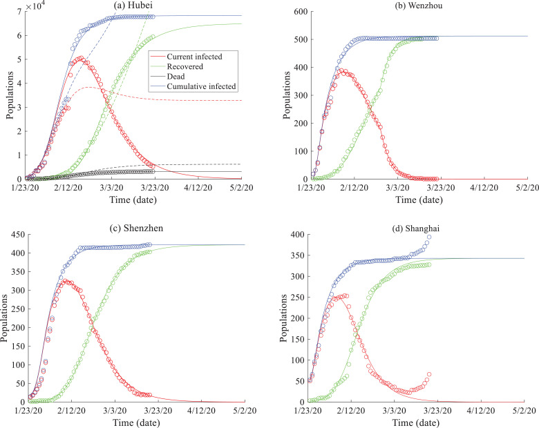
We apply the SEIR model (2) to fit the infection and recovery of coronavirus in China up to 3/7/2020, and then predict the future evolution of COVID-19 spread (Fig. 1 ). The measured time series data of COVID-19 evolution from 3/8/2020 to 3/22/2020 are used to check the model predictions. The epicenter of the infected population in China has been under full lockdown to limit the spread of coronavirus, and hence, the infection dynamics of coronavirus herein represent one under a strict mitigation scenarios for coronavirus.
Fig. 1.
SEIR model results: the observed infection and recovery curves (symbols) versus the solutions of the SEIR model (2) (solid lines) for (a) Hubei province, and the cities of (b) Wenzhou, (c) Shenzhen, and (d) Shanghai in China. In (a), the blue and red dotted lines represent solutions of the constant-parameter SEIR model, and the black dots represent the death toll simulation using the classical PDE .
These tests first show that the best-fit time indexes α 1 ~ α 4 in (2a)~(2d) are all equal to 1, implying that the transmission, infection, and recovery of COVID-19 in China up to 3/22/2020 are not associated with time nonlocal processes. For example, the recovery curve depicted in Fig. 1 does not exhibit any late-time tailing behavior, which supports the application of the integer-order, time-local model (2c). The fast decline of the late time “current infected population” is most likely due to the improvement of health care facilities, which tends to accelerate the recovery of infected people and remove the possible memory impact on the disease recovery evolution.
2.2.1. Comparison of different models
Other complex SEIR models were also applied to model COVID-19 spread, such as the one proposed by Tang et al. [32] which has 12 rates/probabilities and 8 groups of people in SEIR. Numerical results show that, compared with the SEIR model (2), the complex model proposed by Tang et al. [32] (with solutions shown by the dotted lines in Fig. 1a) accurately fits the observed data at the early stage, but then overpredicts the spread of COVID-19 observed after 2/12/2020. The dynamics of transmission for COVID-19, especially the recovery rate, therefore, changed over time in China, likely due to the time-dependent conditions (i.e. improvements/adjustment)s in medical care as mentioned above. A dynamic time-local SEIR model, therefore, may be preferred for modeling COVID-19 spread in China.
In addition, compared to the FDE (2e), the best-fit solution using the classical PDE for death evolution (see the black, dotted line in Fig. 1a) slightly overestimates the late-time growth of mortality. The actual death toll in Hubei province grew slower than that estimated by a constant rate model, indicating that the memory impact may affect the late-time dynamics of death and can be better captured by the FDE (2e).
2.2.2. Comparison of different regions in China
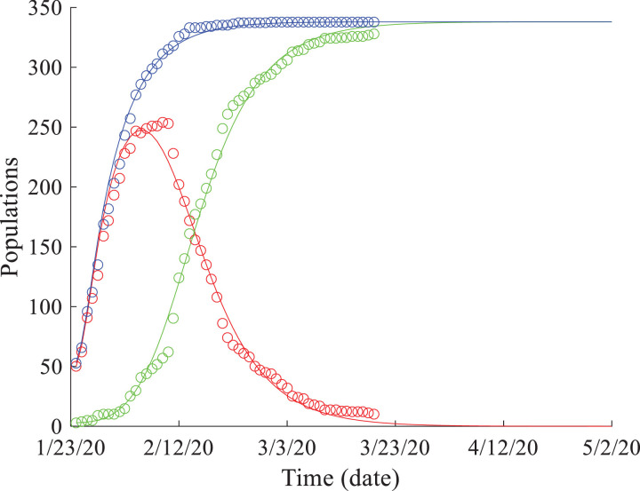
The best-fit solutions using model (2) fit the evolution of the infected and recovered populations well for the data recorded from Hubei province and three large cities closely related (such as in transportation or economic cooperation) to Wuhan, China (Fig. 1). The model was also shown to predict well the observed time series of COVID-19 spread from 3/8/2020 to 3/22/2020 for most places, except for Shanghai City (Fig. 1d). This is likely due to the number of overseas COVID-19 cases imported into Shanghai, whereby the number of cases were observed to increase rapidly after 3/3/2020, causing inconsistency in the affected population and failure of the model. Shanghai Pudong International Airport, one of the two airports located in Shanghai City, is the eighth-busiest airport in the world and the busiest international gateway of mainland China. When excluding the coronavirus cases imported from overseas, model (2) predicts the COVID-19 spread evolution data in Shanghai (Fig. 2 ). Therefore, model (2) works well for various places in China that may not be experience a significant influx of imported cases, as external sources can easily break the internal evolution, especially the asymptotic status, of COVID-19 in China.
Fig. 2.
SEIR model results: the observed COVID-19 spread data (symbols) versus the solutions of model (2) (solid lines) for Shanghai City, China, after deleting the coronavirus cases imported from overseas.
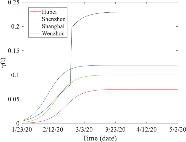
The resultant time-dependent recovery rate γ(t) is depicted in Fig. 3 , where the rate fitted by the latest observation data point within the fitting period (i.e., 3/7/2020) remains stable in the following prediction period. The best-fit recovery rate is the highest for Shanghai (except for the impulse of γ(t) for Wenzhou as discussed below), which is expected since Shanghai has the best public health system of all of these cities. Contrarily, Hubei shows the lowest recovery rate, likely due to its delayed response and the relatively limited public health capability at the beginning of the outbreak compared with Shanghai.
Fig. 3.
Comparison of the time-dependent recovery rate γ(t) fitted for the four areas in China including Hubei province and the cities of Shenzhen, Wenzhou, and Shanghai.
Wenzhou exhibits an impulse in the infection and recovery dynamics of coronavirus (Fig. 1b), different from that observed for the other places studied herein. On February 27, 2020, the number of Wenzhou's infected people suddenly declined, combined with the sudden increase of the number of people cured. This abrupt change can be effectively captured by the SEIR model (2) with an impulse in the recovery rate γ(t). This recovery impulse is most likely due to a new hospital, the No. 2 Affiliated Hospital of Wenzhou Medical University, recently built in this city in early February, which significantly improved the public health system. The first discharged cases of coronavirus from this hospital appeared in late February 2020, resulting in the sudden increase in the total recovery rate. In addition, a relatively large number of people working in Wuhan returned to Wenzhou in late January, and it appears that the improved efficient screening process successfully identified the number of infected cases. The new cases were ~29,000 from 1/24/2020 to 1/31/2020 in Wenzhou (with an average of 3,600 new patients per day), who were then immediately centralized for treatment. It appears that this fast response helped to alleviate the spread of coronavirus in Wenzhou.
2.2.3. Parameter analysis
The best-fit parameters of model (2) are listed in Table 1 , and the initial values for each group of people are listed in Table 2 . We reveal three behaviors in model parameters. First, the best-fit “S”-shaped recovery rate γ(t) (Fig. 3) can be described by the sigmoid function (where a, b, and c are factors), showing that the recovery rate increases exponentially before reaching a stable condition. This increase is likely due to the fact that healthcare facility capabilities improved with time (with an accelerating rate) before reaching their asymptote or maximum capacity.
Table 1.
Best-fit parameters of the SEIR model (2) for Hubei province and three cities in China. The best-fit time indexes α1 ~ α4 in (2a)~(2d) are all equal to 1, and the best-fit time index β in the FDE (2e) is 0.95.
| Place | r | r2 | p | p2 | α | γβ(t) |
|---|---|---|---|---|---|---|
| Hubei province | 10 | 10 | 0.035 | 0.030 | 1/7 | |
| Wenzhou | 15 | 15 | 0.065 | 0.065 | 1/7 | n/a 1 |
| Shenzhen | 10 | 15 | 0.045 | 0.045 | 1/7 | n/a |
| Shanghai | 15 | 15 | 0.065 | 0.065 | 1/7 | n/a |
There was not enough reported data to reliably fit this parameter for this city.
Table 2.
Initial values needed for the SEIR model (2) for Hubei province and three cities in China.
| Place | S(0) | E(0) | I(0) | R(0) | D(0) |
|---|---|---|---|---|---|
| Hubei province | 61,499 | 4007 | 494 | 31 | 24 |
| Wenzhou | 287 | 223 | 0 | 2 | 0 |
| Shenzhen | 338 | 69 | 13 | 2 | 0 |
| Shanghai | 164 | 126 | 50 | 3 | 0 |
Second, the rates and probabilities (r, r 2, p, and p 2) affecting the COVID-19 transmission/infection evolution slightly change in space and remain stable for a given site (Table 1). The small spatial fluctuation of these rates may be due to the similar strategies implemented by local governments for intervening and mitigating COVID-19 spread (i.e., full lockdowns) across the country. The time-invariant transmission/infection rates for a given site indicate that the spreading rate of COVID-19 may not significantly change over a short period of time for a given area with consistent intervening policies enacted.
Third, the model predictions show that it may take 47, 14, 25, and 11 days from 3/14/2020 for the current infected population to drop below 1% of the cumulative infected population for Hubei province, and the cities of Wenzhou, Shenzhen, and Shanghai, respectively. Notably, since the best-fit γ(t) increases in time, the prediction using a constant γ may overestimate the long-term future infection cases and underestimate the future recovery trend for COVID-19.
We also introduce an index C to quantify the infection severity of COVID-19 at different places:
| (3) |
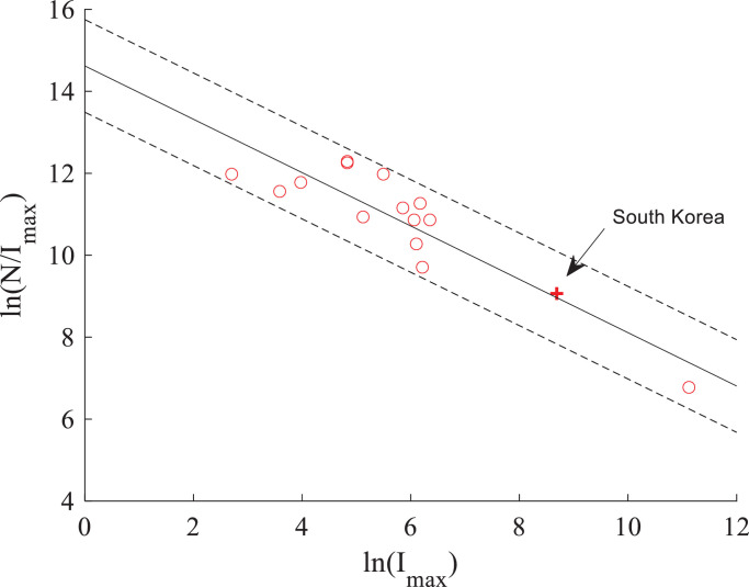
where Imax is the maximum number of cumulative infected people at the given site. A smaller C represents a greater infection severity of coronavirus. There is a power-law relationship between the regional population N and the maximum cumulated number of infected people Imax (Fig. 4 ). This empirical formula may be used to approximate the largest cumulative number of infections, which will be applied in the subsequent section for predicting the COVID-19 evolution outside of China, where the coronavirus infection has not yet reached its peak number of cases.
Fig. 4.
Index of infection severity (C) versus the maximum cumulative number of infections (Imax) calculated for different places in China (circles) and South Korea (the plus symbol). The best-fit relationship (shown by the solid line) is . The dashed lines represent the 95% confidence bounds.
3. Prediction of spreading of COVID-19 in the world
Different countries are applying different modes to slow the the spread of the COVID-19. In the next sub-sections, we discuss several representative countries and then fit/predict the virus spread there.
3.1. United States
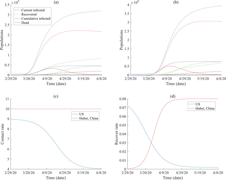
To decrease the acceleration of COVID-19 spread, the U.S.’s main propagated mode up to 3/22/2020 has been the use of social distancing actions. The predicted COVID-19 spread in the U.S. is plotted in Fig. 5 . There is a high uncertainty in the prediction of COVID-19 evolution within the U.S., considering the recent dramatic fluctuations in the number of infected people and the delayed screening during the beginning stages of the outbreak. Thus, we must make assumptions and can only estimate the future coronavirus evolution in the U.S. under specific scenarios. Based on the index of infection severity (C) in the representative areas of China, we predict the U.S. COVID-19 evolution dynamics under two scenarios as shown in Fig. 5.
Fig. 5.
SEIR model results: Predictions of the time series of the infected and recovered population of COVID-19 in (a) California, U.S., and (b) the U.S. The solid lines represent the scenario with virus propagating trend similar to Hubei, China; and the dashed lines represent one scenario with a different contact rate (shown by the blue line in (c)) and recover rate (shown by the blue line in (d)).
Fig. 5a shows the possible spread of COVID-19 in California, U.S., assuming that the coronavirus dynamics (including the infection/recovery rates and the infection severity) are similar to those observed in Hubei, China (the solid lines, representing an optimistic scenario) or can change quite differently (the dashed lines, representing a longer-term, severe scenario). The estimated total population of infection in California varies from 50,000 to 200,000, with the peak number of cases occurring around ~20 to ~50 days from 3/22/2020.
Fig. 5b shows the possible spread of COVID-19 in the U.S. Solid lines represent model solutions assuming that COVID-19 spreads similarly to that as observed in Hubei, China, while the dashed lines are model solutions that assume COVID-19 spreads differently. The results show that the estimated total infected population varies from 700,000 to 3,000,000, with the peak number of cases occurring 20~50 days and the COVID-19 outbreak lasting for >50 days from 3/22/2020, respectively.
3.2. Italy
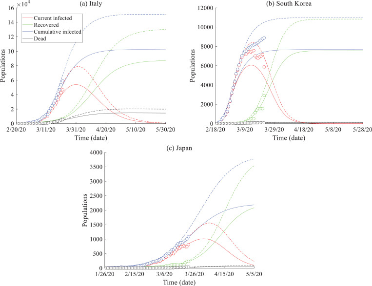
To decrease the acceleration of COVID-19 spread, Italy's mode is now similar to China: lockdown of the full population. The predicted COVID-19 spread in Italy is plotted in Fig. 6 a. Although Italy has followed China's mode of national isolation, the number of infected people increased rapidly from 3/14/2020 to 3/19/2020 (~495 new cases per day). To account for the delayed national quarantine compared with China, we decrease the C index (while also increasing the upper limit of the cumulative infection). The COVID-19 evolution prediction results show that there may be a turning point in the next two weeks when the current infected cases begin to decline. We also separate the death toll from the number of recovered cases.
Fig. 6.
SEIR model results: Prediction of COVID-19 spread in different regions in the world (with the measured data up to 3/22/2020): (a) Italy, (b) South Korea, and (c) Japan. Data sources are from [1].
3.3. South Korea
South Korea's mode of combating the spread of COVID-19 is through fast detection and tracking of the disease. South Korea is using efficient mobile diagnoses tests and accurate tracing of infected cases to maintain a low death rate even with a large infected population. The mobile method can test 20,000 people per day (the maximum capability on 3/12/2020), and apps for cell phones and/or credit cards can accurately track the routes of infected people with the help of local government (without an invasion of privacy), so that warnings can be immediately delivered to the general population to obviate the places with high risk. The current infected population may have passed its peak number of cases around 3/20/2020, and the prediction shows that the COVID-19 outbreak may be well controlled in ~35 days from 3/22/2020 (Fig. 6b).
3.4. Japan
Japan's mode of combating the spread of COVID-19 is compatible with that of the U.S., in addition to other changes such as enhanced education/outreach and rapid treatment of the infected cases. Specific policies include social distancing (which might be a key barrier to the spread of the novel coronavirus), personal hygiene, and quarantine of the infected cases. The current data and modeling results (Fig. 6c) show that Japan has an efficient way so far to limit the maximum population infected and slow the spread of COVID-19, while this outbreak may last for a while.
4. Stochastic model to evaluate scenarios to mitigate the outbreak of COVID-19 in a city
The model-predicted COVID-19 spread in the U.S., using the fitted infection and recovery rates from China (Fig. 5), reveals the impact of one possible mitigation scenario for COVID-19: coronavirus lockdowns, which have now been implemented by some states in the U.S. such as California and New York. Other non-pharmaceutical options can and should also be evaluated using mathematical models, considering the recent surge of infected cases in the U.S.
When the number of infected persons is initially small compared to that of susceptible people, the infected and susceptible people are not well mixed and hence the system is not homogeneous. Under such conditions, a stochastic model is needed, as the deterministic, continuum models (such as the SEIR model) assume well-mixing of components for a homogeneous system [33,34]. Hence, this section develops and applies a stochastic model to evaluate non-pharmaceutical scenarios for mitigating the COVID-19 with a small number of initial infections.
4.1. Stochastic model development
The random walk based stochastic model for COVID-19 spread is analogous to a mixing-limited bimolecular reaction-based mechanism/condition [35]. When a reactant A particle (representing a susceptible individual A) meets a reactant B particle (representing an infectious person B), a chemical reaction may occur if the collision energy is large enough to break the chemical bond (meaning that the susceptible person A may be infected if satisfying additional criteria such as A and B are close enough, and B touches his/her face after receiving coronavirus from A). Therefore, the condition of A being infected is not deterministic but rather a random, probability-controlled process. This probability is related to various factors, such as the duration that A and B are in contact, the infectivity rate, and the distance between the two people, which may be characterized parsimoniously by the interaction radius R that controls the number of reactant pairs (susceptible + infectious) in a potential reaction (infection) [35]. Hence, the core of the random walk stochastic model to simulate COVID-19 spread is to define the interaction radius R.
The analogous development and similarities between bimolecular reactions and the SIR model can also be seen from their governing equations. The time-dependent SIR model takes the form [36]:
| (4a) |
| (4b) |
| (4c) |
| (4d) |
where β(t) and γ(t) denote the transmission rate and recovery rate at time t, respectively.
The rate equations for irreversible bimolecular reaction take the form [35]:
| (5a) |
| (5b) |
| (5c) |
where [A], [B], and [C] denote the concentrations of A, B, and C, respectively; and Kf(t) is the forward kinetic coefficient of reaction. Equations (5a) and (5b) are functionally similar to equations (4a) and (4b), respectively, if the recovery rate . Therefore, following the argument in Zhang et al. [35] and Lu et al. [37], we derive analytically the interaction radius R for the SIR model (4):
| (6) |
where V denotes the volume of the domain, Δt is the time step in random walk particle tracking, is the mass (or weight) carried by each A particle, [A 0] is the initial concentration of A (which can be assumed to be the normalized value 1 here), and denotes the initial number of susceptible people.
The movement of A, B, and C can be described by the following time FDE [35]:
| (7) |
where denotes A, B, and C, respectively; β* denotes the fractional capacity coefficient (which controls the ratio between the immobile and mobile population); v denotes the mean moving speed; and D denotes the macrodispersion coefficient.
After defining the interaction radius R, the particle tracking scheme proposed by Zhang et al. [35] and Lu et al. [37] with particle trajectories defined by the time FDE (7) can be applied to model the transmission of coronavirus between the susceptible and infectious people.
4.2. Scenario evaluation to mitigate the COVID-19 outbreak in a city
In addition to pharmaceutical strategies including vaccine and therapeutic drug development, and herd immunity that may either take a while or have a high risk, non-pharmaceutical scenarios can be tested. Several particle-tracking based stochastic models were proposed recently [38] to evaluate non-pharmaceutical scenarios to mitigate coronavirus spreading in a city. Here we evaluate three related scenarios (described below) using the stochastic model proposed above.
Scenario 1: No special constraints. Assuming a city with 10,000 people and 4 initial coronavirus cases. This scenario does not put any constraints for any population. We assume that the population distributes in the city randomly at the beginning, and then moves randomly. The spread of COVID-19 is then simulated using the stochastic model proposed in Section 4.1.
Scenario 2: Social distancing. This scenario assumes that all people in the city maintain a social distance, significantly decreasing the probability of infection.
Scenario 3: Attempted quarantine. This scenario creates a forced quarantine for infected individuals before the outbreak (which is expected to be the most efficient way of quarantine).
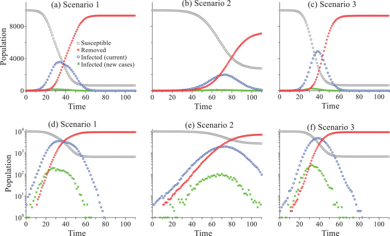
In the stochastic model, we assume that 10 days after being infected, the person will be removed because of being cured or expired (dead). This is because the median disease incubation period has been estimated to be 5.1 days [39]. For simplicity purposes, the interaction radius R (6) remains constant, since the constant interaction radius was found to be able to efficiently capture the temporal variation of effective reaction rates in mixing controlled reaction experiments or simulations [35,37]. The initial number of A and B particles is 10,000 and 4, respectively. The Lagrangian solutions of the COVID-19 outbreak for the three scenarios are depicted in Fig. 7 .
Fig. 7.
Stochastic modeling: the simulated virus spread in the city using the Lagrangian approach for the three mitigation scenarios: Scenario 1 (a), Scenario 2 (b), and Scenario 3 (c). The bottom plot is the semi-log version of the top plot, to show the tails of each curve.
Modeling results for scenarios 1, 2, and 3 show a peak in the curve of newly infected people at time t=28, 65, and 32, respectively, demonstrating that the virus spreads the fastest for the scenario without mitigation constraints (i.e., scenario 1, where the number of the total infected people or cases increases by one order of magnitude every 10 days in the rising limb), as expected. However, the value for this peak (scenario 1, =198 people) is lower than that for scenario 3 (=267 people), although the total number of the infected people for scenario 1 (9,336) is slightly larger than scenario 3 (9,322). This may be due to a greater separation of infection cases for the higher number of initial coronavirus carriers in scenario 1, which causes a lower and relatively flatter COVID-19 evolution peak compared to that of scenario 3. Scenario 2 has the lowest peak value (=121 people) and the most-delayed peak in the curve for new cases, and the total infection time is almost doubled compared to the other two scenarios, indicating that people living with strict social distancing may also suffer from a much longer period of COVID-19 threat. It is also noteworthy that the overall trend of the solution (simulation) of scenario 1 (initial surge without special constraints, Fig. 7a) is similar to that for Italy which had a delayed response to the COVID-19 outbreak initially (Fig. 6a), and scenario 3 solution (a lower peak value and a longer duration due to social distancing, Fig. 7b) is similar to that observed in Japan where social distancing actions have been implemented (Fig. 6c).
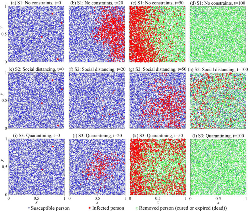
The simulated particle plumes plotted in Fig. 8 reveal the subtle discrepancy between the three mitigation scenarios. Scenario 1 assumes that four initial cases were initially located on the right side of the city, while the whole population (10,000 susceptible persons) was distributed randomly in the 1 × 1 domain (Fig. 8a). The trajectory of each person is assumed to follow (two-dimensional) Brownian motion with retention (described by Eq. (7)), to capture the random vector for each displacement and the random waiting time between two consecutive motions (described by the time fractional derivative term in Eq. (7)). The virus moved quickly from east to west (Figs. 8b and 8c), spreading over the entire city before all the infected people were cured or expired (dead) at time t=69 (Fig. 8d). A total of 664 susceptible people (6.6% of the total population) distributed randomly around the city were never infected.
Fig. 8.
Stochastic modeling: the simulated particle plumes at different times (t=0, 20, 50, and 100 at the 1st, 2nd, 3rd, and 4th columns) for three scenarios to mitigate the COVID-19 outbreak in a city: Scenario 1 (S1): no constraint (1st row) (a)~(d), Scenario 2 (S2): Social distancing (2nd row) (e)~(h), and Scenario 3 (S3): Quarantining (3rd row) (i)~(l).
Scenario 2 assumes that social distancing can reduce the infection probability, which can be characterized by a smaller reaction rate or a smaller interaction radius in our Lagrangian approach. The virus was spreading at a much lower rate from west to east than that in scenario 1 (Figs. 8e 8g), reaching a stable condition (i.e., # of cases neither increasing or decreasing) at a later time (t=125) and leaving more susceptible people unaffected (2,734 total, which is 27.3% of the population). Therefore, social distancing is effective in limiting the spread of coronavirus among people. Note, however, this scenario assumes that every person in this city strictly maintains social distancing; otherwise a surge of infections may occur the same way as that shown in scenario 1.
Scenario 3 assumes self-quarantine. Notably, not all of the infected people can be effectively quarantined due to the following: 1) people can be infected without coronavirus symptoms; 2) people in the incubation period can transmit the infection; and 3) limited health care facilities and capabilities for the large influx of patients. For example, according to Imai et al. [40], many infected people could not be appropriately screened initially in Wuhan City, China. Under this condition, we assume that 50% of people infected and diagnosed are immediately quarantined, while the remaining infected people (Fig. 8i) can still cause the spread of coronavirus (Figs. 8j 8l). Self-quarantine, therefore, may not be as effective as maintained social distancing.
5. Conclusions
Fractional calculus provides a useful tool to modeling complex dynamics in biology, and this study extended the FDE for modeling the coronavirus outbreak. The COVID-19 is a pandemic radically impacting our lives by altering our daily patterns and interactions in an unprecedented way and rate. A time-dependent SEIR model with built-in FDE components, motivated by the coronavirus milestone of recording zero new local infections in China on 3/19/2020, was applied to capture the COVID-19 evolution observed over the last three months in China. A stochastic model built upon the time FDE for random resting times of people was also proposed to evaluate non-pharmaceutical mitigation options. Three main conclusions are presented by this study.
First, different properties in the COVID-19 spreading in China (data up to 3/22/2020) exhibited different kinetics, and the death evolution can be captured by the time FDE. Model fitting showed that the recovery rate of COVID-19 increases with time due to various human factors. The fast-increasing recovery rate caused the rapid decline of the “current infected population” curve, removing the possible memory impact and any delayed processes, which does not require a time-nonlocal model such as the time FDE. Contrarily, the evolution of deaths in China, Italy, South Korea, and Japan can be captured well by the time FDE, likely due to the time memory in the death toll. It is also noteworthy that the time FDE version of the SEIR model might be needed if the late-time recovery rate declines due to the change of coronavirus properties affected by the change of climate, public policy, and/or possible evolution of the virus itself and the contiguous manner/rate.
Second, the updated SEIR model provided predictions, although with high uncertainty, for COVID-19 evolution within China and for other countries. For example, the improved SEIR model showed that, if the infection and recovery rates remain stable, the number of cumulative infections is likely to decline to 1% of the total infected population within one month (from 3/22/2020) in China. The overseas imported cases, however, may break the internal asymptotic status and significantly postpone the ending time of COVID-19 in China. Predictions using the validated SEIR model also showed different evolution dynamics of COVID-19 within populations of the United States, Italy, Japan, and South Korea. For example, it may take at least 2~3 months for the current infected population to drop below 1% of the cumulative infected population in the U.S. (requiring more efficient mitigation strategies), while South Korea may control the COVID-19 spread in a relatively shorter period. However, these predictions contain high uncertainty due to uncertainty in the maximum infected population, and changes of transmission/infection and recovery rates among different countries.
Third, a stochastic model based on the Lagrangian scheme for the time FDEs, analogous to a mixing-limited reaction mechanism model, showed that self-quarantine may not be as effective as strict social distancing, since not all the infected people can be diagnosed and immediately quarantined. While strict social distancing can apparently slow COVID-19 spread, the pandemic may last longer. This is another case that fractional calculus may be used to explore COVID-19 outbreak. Therefore, one of the main contributions of this study is to extend the application of FDEs to model dynamics and mitigation scenarios of the coronavirus spread.
CRediT authorship contribution statement
Yong Zhang: Conceptualization, Methodology, Software, Writing - original draft, Writing - review & editing. Xiangnan Yu: Data curation, Methodology, Software, Visualization. HongGuang Sun: Supervision. Geoffrey R. Tick: Data curation, Formal analysis. Wei Wei: Resources. Bin Jin: Funding acquisition, Supervision.
Declaration of Competing Interest
The authors declare that they have no known competing financial interests or personal relationships that could have appeared to influence the work reported in this paper.
Acknowledgement
X.Y. was partially funded by the Fundamental Research Funds for the Central Universities (under grant 2019B66814 and 2019B16014) and Postgraduate Research & Practice Innovation Program of Jiangsu Province (under grant SJKY19_0423), W.W. and H.S. were partially funded by the National Natural Science Foundation of China (under grants 41931292 and 11572112). This paper does not necessarily reflect the views of the funding agency. The authors would also like to thank Dr. Bingqing Lu and Mr. Xiaoting Liu for collecting part of the data and literature.
Footnotes
For submission to Chaos, Solitons and Fractals, Special issue on “Recent Advances in Computational Biology”.
Appendix: Impacts of the non-singular kernel and the fractional derivative type on model results
This appendix quantifies the potential impacts of the non-singular kernel and the type of the fractional derivative on the COVID-19 death toll simulation. First, the nonsingular time-fractional definitions also provde promising modeling tools for real-world fractional dynamics. For example, the Atagana-Baleanu fractional derivative is defined as [41]:
| (8) |
where represents the single-parameter Mittag-Leffler function.
We employ this definition to extend the SEIR model and then use the finite difference method to simulate the evolution of the COVID-19 death toll, which leads to the following solver:
where E β, α(t) represents the double-parameter Mittag-Leffler function with ; τ denotes the (uniform) time interval of the finite difference scheme; and D (j) stands for the number of death at the j-th time, i.e., .
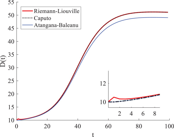
We then compare this definition with the Caputo and Riemann-Liouville fractional derivatives under the same condition. Results show that the new definition (8) describes the evolution of the COVID-19 related death toll with a stronger memory effect than the power-law kernel function (Fig. 9 ), which is consistent with the conclusion in the previous study (see [42]). The resultant death roll peak is lower than that simulated by the conventional kernel function, but it does not mean that the kernel used in the Caputo fractional derivative is no longer valid. Indeed, the solution of the Caputo fractional derivative can capture well the obsvered death peak (Fig. 1a). Applications of the nonsingular kernel functions deserve further study in the future.
Fig. 9.
Comparison of the evolution of the COVID-19 death toll estimated by the SEIR model with different fractional derivatives. The initial condition is taken as (the y-axis “D(t)” denotes the temporal evolution of the death toll), and the fractional order . The Caputo solution (the black dashed line) is almost identical to the Riemann-Liouville solution (the red line), except for the early time shown in the inset.
Second, the Riemann-Liouville fractional derivative is defined as [43]:
| (9) |
The Caputo fractional derivative listed in Section 2.1 and the Riemann-Liouville fractional derivative (9) are related by [44]:
where 0 < β < 1, and the operators and represent the Caputo and Riemann-Liouville fractional derivatives, respectively.
Fig. 9 compares solutions of these two fractional derivatives. The resultant death toll of COVID-19 cases for the Caputo definition is almost identical to the Riemann-Liouville solution, except for that at the early time. The solution of the Riemann-Liouville derivative near t = 0 is unexpected higher than that of the Caputo one, and the Caputo definition is more consistent with the real-world data. Hence, it is valid to use the Caputo fractional derivative in this study.
References
- 1.Lonescu C, Lopes A, Copot D, Machado JAT, Bates JHT. The role of fractional calculus in modeling biological phenomena: A review. Commun Nonlinear Sci Numer Simulat. 2019;51:141–159. [Google Scholar]
- 2.Magin RL. Fractional calculus models of complex dynamics in biological tissues. Comput Math Appl. 2010;59(5):1586–1593. [Google Scholar]
- 3.Atici FM, Sengul SS. Modeling with fractional difference equations. J Math Anal Appl. 2010;369(1):1–9. [Google Scholar]
- 4.Machado JAT, Costa AC, Quelhas MD. Fractional dynamics in DNA. Commun Nonlinear Sci Numer Simul. 2011;16(8):2963–2969. [Google Scholar]
- 5.Petras I, Magin RL. Simulation of drug uptake in a two compartmental fractional model for a biological system. Commun Nonlinear Sci Numer Simul. 2011;16(12):4588–4595. doi: 10.1016/j.cnsns.2011.02.012. [DOI] [PMC free article] [PubMed] [Google Scholar]
- 6.Rihan FA, Baleanu D, Lakshmanan S, Rakkiyappan R. On fractional SIRC model with salmonella bacterial infection. Abstr Appl Anal. 2014;2014 doi: 10.1155/2014/136263. [DOI] [Google Scholar]
- 7.Shaha K, Alqudah MA, Jarad F, Abdeljawa T. Semi-analytical study of Pine Wilt Disease model with convex rate under Caputo-Febrizio fractional order derivative. Chaos Soliton Fract. 2020;135 [Google Scholar]
- 8.Jajarmi A, Yusuf A, Baleanu D, Inc M. A new fractional HRSV model and its optimal control: A non-singular operator approach. Physica A. 2020;547 [Google Scholar]
- 9.Baleanu D, Jajarmi A, Sajjadi SS, Asad JH. The fractional features of a harmonic oscillator with position-dependent mass. Commun Theor Phys. 2020;72(5) [Google Scholar]
- 10.Baleanu D, Jajarmi A, Mohammadi H, Rezapour S. A new study on the mathematical modelling of human liver with Caputo-Fabrizio fractional derivative. Chaos Soliton Fract. 2020;134 [Google Scholar]
- 11.Yildiz TA, Jajarmi A, Yildiz B, Baleanu D. New aspects of time fractional optimal control problems within operators with nonsingular kernel. Discrete Cont Dyn. 2020;13(3):407–428. [Google Scholar]
- 12.Baleanu D, Jajarmi A, Sajjadi SS, Mozyrska D. A new fractional model and optimal control of a tumor-immune surveillance with non-singular derivative operator. Chaos. 2019;29(8) doi: 10.1063/1.5096159. [DOI] [PubMed] [Google Scholar]
- 13.Johns Hopkins Coronavirus Resource Center, 2020. https://coronavirus.jhu.edu/map.html
- 14.Yang C, Wang J. A mathematical model for the novel coronavirus epidemic in Wuhan. China. Math Biosci Eng. 2020;17:2708–2724. doi: 10.3934/mbe.2020148. [DOI] [PMC free article] [PubMed] [Google Scholar]
- 15.del Rio C, Malani PN. COVID-19 – New insights on a rapidly changing epidemic. JAMA. 2020 doi: 10.1001/jama.2020.3072. [DOI] [PubMed] [Google Scholar]
- 16.Hellewell J, Abbott S, Gimma A, Bosse NI, Jarvis CI, Russell TW, Munday JD, Kucharski AJ, Edmunds WJ. Feasibility of controlling COVID-19 outbreaks by isolation of cases and contacts. Lancet Glob Health. 2020;8:e488–e496. doi: 10.1016/S2214-109X(20)30074-7. [DOI] [PMC free article] [PubMed] [Google Scholar]
- 17.Kermack WO, McKendrick AG. A contribution to the mathematical theory of epidemics. P Roy Soc A Math Phys Eng Sci. 1927;115:700–721. [Google Scholar]
- 18.Peng L, Yang W, Zhang D, Zhuge C, Hong L. Epidemic analysis of COVID-19 in China by dynamical modeling. 2020, https://arxiv.org/abs/2002.0656
- 19.Li XH, Zhao X, Sun YH. The lockdown of Hubei province causing different transmission dynamics of the novel coronavirus (2019-ncov) in Wuhan and Beijing. medRxiv. 2020 https://www.medrxiv.org/content/10.1101/2020.02.09.20021477.full.pdf [Google Scholar]
- 20.Chen YC, Lu PE, Chang CS. A time-dependent SIR model for COVID-19. 2020, https://arxiv.org/ftp/arxiv/papers/2003/2003.00122.pdf. [DOI] [PMC free article] [PubMed]
- 21.Wang LL, Zhou Y, He J, Zhu B, Wang F, Tang L, Eisenberg M, Song PXK. An epidemiological forecast model and software assessing interventions on COVID-19 epidemic in China. 2020, https://www.medrxiv.org/content/10.1101/2020.02.29.20029421v1.full.pdf.
- 22.Pan J, Yao Y, Liu Z, Li M, Wang Y, Dong W, Kan H, Wang W. Effectiveness of control strategies for Coronavirus Disease 2019: a SEIR dynamic modeling study. 2020. https://www.medrxiv.org/content/medrxiv/early/2020/03/03/2020.02.20.20023572.full.pdf.
- 23.Shi PP, Cao S, Feng P. SEIR Transmission dynamics model of 2019 nCoV coronavirus with considering the weak infectious ability and changes in latency duration. 2020. 10.1101/2020.02.16.20023655. [DOI]
- 24.Wu JT, Leung K, Leung GM. Nowcasting and forecasting the potential domestic and international spread of the 2019-nCoV outbreak originating in Wuhan, China: a modelling study. Lancet. 2020;395:689–697. doi: 10.1016/S0140-6736(20)30260-9. [DOI] [PMC free article] [PubMed] [Google Scholar]
- 25.Zhou T, Liu Q, Yang Z, Liao J, Yang K, Bai W, Lu X, Zhang W. Preliminary prediction of the basic reproduction number of the Wuhan novel coronavirus 2019‐nCoV. J Evidence-Based Med. 2020;13:3–7. doi: 10.1111/jebm.12376. [DOI] [PMC free article] [PubMed] [Google Scholar]
- 26.Chinazzi M, Davis JT, Ajelli M, Gioannini C, Litvinova M, Merler S, Piontti AP, Mu K, Rossi L, Sun K, Viboud C, Xiong X, Yu H, Halloran ME, Jr Longini. I M, Vespignani A. The effect of travel restrictions on the spread of the 2019 novel coronavirus (COVID-19outbreak. Science. 2020:eaba9757. doi: 10.1126/science.aba9757. 06 Mar 2020. [DOI] [PMC free article] [PubMed] [Google Scholar]
- 27.Boldog P, Tekeli T, Vizi Z, Dénes A, Bartha FA, Rost G. Risk assessment of novel coronavirus COVID-19 outbreaks outside China. J Clin Med. 2020;9:571. doi: 10.3390/jcm9020571. [DOI] [PMC free article] [PubMed] [Google Scholar]
- 28.Hilton J, Keeling MJ. Estimation of country-level basic reproductive ratios for novel Coronavirus (COVID-19) using synthetic contact matrices. 2020, https://www.medrxiv.org/content/10.1101/2020.02.26.20028167v1. [DOI] [PMC free article] [PubMed]
- 29.Brauer F, Castillo-Chavez C, Castillo-Chavez C. Vol. 2. Springer; New York, U.S.: 2012. pp. 3–47. (Mathematical Models in Population Biology and Epidemiology). [Google Scholar]
- 30.Caputo M. Linear model of dissipation whose q is almost frequency independent-II. Geophys J Int. 1967;13:529–539. [Google Scholar]
- 31.Zhang Y, Yu XN, Li XC, Kelly JF, Sun HG, Zheng CM. Impact of absorbing and reflective boundaries on fractional derivative modes: Quantification, evaluation and application. Adv Water Resour. 2019;128:129–144. [Google Scholar]
- 32.Tang B, Wang X, Li Q, Bragazzi NL, Tang S, Xiao Y, Wu JH. Estimation of the transmission risk of the 2019-nCoV and its implication for public health interventions. J Clin Med. 2020;9:462. doi: 10.3390/jcm9020462. [DOI] [PMC free article] [PubMed] [Google Scholar]
- 33.Allen LJS. 2nd ed. CPC Press; New York, U. S.: 2010. An introduction to stochastic processes with applications to biology; pp. 45–102. [Google Scholar]
- 34.Chalub FACC, Souza MO. Discrete and continuous SIS epidemic models: A unifying approach. Ecol Complex. 2014;18:83–95. [Google Scholar]
- 35.Zhang Y, Papelis C, Sun P, Yu Z. Evaluation and linking of effective parameters in particle-based models and continuum models for mixing-limited bimolecular reactions. Water Resour Res. 2013;49:4845–4865. [Google Scholar]
- 36.Newman M.Networks: An Introduction. Oxford University Press, 2010.
- 37.Lu BQ, Zhang Y, Sun HG, Zheng CM. Lagrangian simulation of multi-step and rate-limited chemical reactions in multi-dimensional porous media. Water Sci Eng. 2018;11:101–113. [Google Scholar]
- 38.Stevens H.Why outbreaks like coronavirus spread exponentially and how to “flatten the curve”. The Washington Post, March14, 2020. https://www.washingtonpost.com/graphics/2020/world/corona-simulator/
- 39.Stephen AL, Grantz KH, Bi O, Jones FK, Zheng O, Meredith HR, Azman AS, Reich NG, Lessler J. The Incubation Period of Coronavirus Disease 2019 (COVID-19) From Publicly Reported Confirmed Cases: Estimation and Application. Ann Intern Med. 2020 doi: 10.7326/M20-0504. [DOI] [PMC free article] [PubMed] [Google Scholar]
- 40.Imai N, Dorigatti I, Cori A, Donnelly C, Riley S, Ferguson NM. Imperial College London COVID-19 Response Team; China: 2020. Report 2: Estimating the potential total number of novel Coronavirus cases in Wuhan City.https://www.imperial.ac.uk/media/imperial-college/medicine/sph/ide/gida-fellowships/Imperial-College-COVID19-update-epidemic-size-22-01-2020.pdf [Google Scholar]
- 41.Atangana A, Baleanu D. New Fractional Derivatives with Nonlocal and Non-Singular Kernel: Theory and Application to Heat Transfer Model. Thermal Sci. 2016;20(2):763–769. [Google Scholar]
- 42.Yu XN, Y Zhang, Sun HG, Zheng CM. Time fractional derivative model with Mittag-Leffler function kernel for describing anomalous diffusion: Analytical solution in bounded-domain and model comparison. Chaos Soliton Fract. 2018;115:306–312. [Google Scholar]
- 43.Samko SG, Kilbas AA, Marichev OI. Fractional integrals and derivatives. Theory and Applications, Gordon and Breach, Yverdon. 1993:44. [Google Scholar]
- 44.Meerschaert MM, Sikorskii A. Stochastic models for fractional calculus. Walter de Gruyter. 2011:43. [Google Scholar]


