A Primer on COVID‐19 Mathematical Models

The emergence of severe acute respiratory syndrome coronavirus 2 (or coronavirus disease [COVID]‐19) has led to a widespread global pandemic (1). COVID‐19 symptoms and mortality are disproportionately more severe in people with obesity and obesity‐related comorbidities (2, 3). This is of concern for the United States, where ~42% have obesity, and of these, 85% have type 2 diabetes.

Without effective vaccines or therapies, there is an urgent need for prevention and treatment strategies for COVID‐19 infections. Developing such strategies requires a thorough understanding of how COVID‐19 infections spread in a population. Mathematical modeling predicts the spread of COVID‐19 and permits testing different strategies to control and reduce population disease impacts.

The New York Times published COVID‐19 predictions from five mathematical models with widely varying results (4). A recent review (5) also highlighted model differences and noted that a fluid situation dependent on many external variables should not be viewed as a “crystal ball.” Why do COVID‐19 models yield such variable predictions? How are the different COVID‐19 models developed? How should models be applied? Here, we provide a brief tutorial addressing these questions.

The majority of models fall into the following two categories, which are applied for different purposes: projections versus statistical forecasts. Projections are deterministic and they explain what could happen under a set of underlying hypotheses, while statistical forecasts use observed data to predict what will happen (6).

Dynamic Projection Models

In 1927, Kermack and McKendrick (7) developed the first continuous variable projection model of epidemic population dynamics, often referred to as a “susceptible, infected, and removed” (SIR) model. They compartmentalized a constant population into three states. The first state represents individuals susceptible to the disease with the number of susceptible individuals on day $t$ of the epidemic, denoted by $S\left(t\right).$ The second state is the number of infected individuals on day $t$ of the epidemic, denoted by $I\left(t\right).$ Finally, individuals removed from the infectious disease dynamics through death or recovery with immunity on day $t$ of the epidemic are denoted by $R\left(t\right).$

R models assume susceptible individuals contract the infection by interacting with infected individuals. The term that models this interaction is represented as a proportion of the product of the susceptible and infected: $rS\left(t\right)I\left(t\right)$. If the mortality/recovery rate is modeled as a direct proportion of infected individuals, we arrive at the final Kermack‐McKendrick Model. This flow diagram is depicted in Figure 1, with mathematical formulation as a system of three ordinary differential equations:

$$\frac{\mathit{dS}}{\mathit{dt}}=-rS\left(t\right)I\left(t\right)$$

$$\frac{\mathit{dI}}{\mathit{dt}}=rS\left(t\right)I\left(t\right)-\gamma I\left(t\right)$$

$$\frac{\mathit{dR}}{\mathit{dt}}=\gamma I\left(t\right)$$

Figure 1.

Transition from the three possible states, susceptible $S\left(t\right),$ infected, $I\left(t\right)$, and removed $R\left(t\right).$ The proportion of interactions between individuals in $S\left(t\right)$ and $I\left(t\right)$ that lead to infection per unit time is $r$, and the proportion of infected individuals that recover with immunity or die from disease per unit time is $\gamma$. The total number of individuals within the system remains constant throughout calculation.

The key property of projection models like the Kermack‐McKendrick system is that they are based on logical assumptions of the underlying mechanics of a process and they can be developed without data to immediately address “what if” questions.

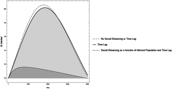
It is from SIR‐like models that we can see the effects of social distancing on flattening the curve. SIR models, however, are sensitive to underlying model assumptions. When these assumptions are modified, projections sometimes change dramatically. For example, we could assume there is a time lag to infection that accounts for the virus incubation period by modifying the term $rS\left(t\right)I\left(t\right)$ to $rS\left(t\right)I\left(t-\tau \right)$. The transmission rate, $r$, could also be assumed dependent on the currently observed infected population. Additionally, instead of assuming $r$ is constant, we could model $r$ as a function of $I\left(t\right)$ by using the Hill function (8) as follows:

$$r\left(I\left(t\right)\right)=\frac{{\mathrm{\beta }}_{max}{K}^n}{I{\left(t\right)}^n+K^n}$$

Here, r declines as the number of infected individuals gets higher, reflecting increased social distancing during peak infectivity. On the other hand, $r$ increases when the number of infected individuals decrease. The values ${\mathrm{\beta }}_{max}$, K, and n are parameters that could be fit to data once available. The changes in assumptions alter the projections as depicted in Figure 2.

Figure 2.

Varying assumptions can alter the dynamic projection model outcomes. Assuming there is a time lag shifts the curve. Including social distancing that increases with increased infective populations and decreases with declining infected populations “flattens the curve” and results in an asymmetric projection. The parameter values were set with total population set as 1,000 individuals, $r=0.02,\gamma =0.01$. For the time lag model, the time lag for infection was set at $\tau =7$ days and the time lag to mortality at 3 days. For the model where $r$ is represented by the Hill function, $K=30,{\beta }_{\mathit{max}}=0.85$ and $n=3.1$.

Once data is fit to model parameters, SIR models can predict when infections peak or how high the peak may be, but as pointed out in Jewell et al. (5) and observed in Figure 2, these are dependent on the underlying model assumptions.

Forecasting Models

Forecasting models are more useful after data has been gathered. For instance, most SIR COVID‐19 models use fixed parameters, which lead to a constant referred to as $R_0$ or “ $R$ naught.” $R_0$ is defined as the number of secondary infections that will result from a single infected individual being introduced into a completely susceptible population. A calculated reproduction number during an ongoing epidemic is the “effective” reproduction number, $R_E\left(t\right)$, which is the observed average number of secondary cases from a single primary case per unit time. $R_E\left(t\right)$ accounts for changes to $R_0$ through control measures such as social distancing.

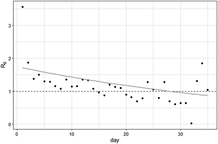
Within the SIR framework, $R_0=rNT$, where $T$ is the time to recover and $N$ is the population size. Absent of interventions, the estimated $R_0$ of COVID‐19 is between 1.5 and 6.7 (9). However, this value is not constant but changing daily. Renewal equations allow us to estimate values (10) of $R_E\left(t\right)$ that can be fit to a statistical model. Similar to Massad et al. (6), we fit an exponential decay model to New York’s data yielding $R_E\left(t\right)=e^{0.5-0.02t}$, though other statistical models such as one with an asymptote could be considered. Figure 3 depicts the fitted effective reproduction number versus the calculated $R_E\left(t\right)$ values for New York. This forecast model will inform improved SIR model projections and generate prediction intervals. Projection models for the SARS‐1 epidemic overestimate $R_0$ compared with statistical forecasting estimates of reproduction numbers (6). It is important that researchers use projection models for hypothetical scenario development and statistical forecasting models for forecasting, which are two different goals.

Figure 3.

The effective reproduction number $R_E\left(t\right)$, sometimes referred to as $R_0$ or “R naught,” for New York fit to data with an exponential curve. $R_E\left(t\right)$ represents the average number of secondary cases because of one infected person at the beginning of the epidemic, and in order for the epidemic to decline, $R_E\left(t\right)$ should be less than 1. The points are the calculated daily effective reproduction number calculated by number of observed cases divided by the number of expected cases on a given day, while the gray curve forecasts future effective reproduction numbers that can be used in dynamic projection SIR models. Here, $R_E\left(t\right)$ went below 1 (represented by the dashed line) around 28 days.

Including the differential effects of COVID‐19 on individuals with obesity into both projection and forecasting models by separating each compartment into normal weight and obesity populations will be key to understanding the population‐wide impacts of COVID‐19 on obesity. Obesity researchers can apply both types of models to evaluate prevention and treatment strategies for COVID‐19 in persons with obesity.

References

- 1. Lai CC, Shih TP, Ko WC, Tang HJ, Hsueh PR. Severe acute respiratory syndrome coronavirus 2 (SARS‐CoV‐2) and coronavirus disease‐2019 (COVID‐ 19): The epidemic and the challenges. Int J Antimicrob Agents 2020;55:105924. doi:10.1016/j.ijantimicag.2020.105924 [DOI] [PMC free article] [PubMed] [Google Scholar]
- 2. Ryan DH, Ravussin E, Heymsfield S. COVID 19 and the patient with obesity ‐ the editors speak out Obesity (Silver Spring). 2020;28:847. [DOI] [PMC free article] [PubMed] [Google Scholar]
- 3. Richardson S, Hirsch JS, Narasimhan M, et al. Presenting characteristics, comorbidities, and outcomes among 5700 patients hospitalized with COVID‐19 in the New York City area. JAMA 2020;323:2052‐2059. [DOI] [PMC free article] [PubMed] [Google Scholar]
- 4. Bui Q, Katz J, Parlapiano A, Sanger‐Katz M. What 5 coronavirus models say the next month will look like. New York Times. April 20, 2020. [Google Scholar]
- 5. Jewell NP, Lewnard JA, Jewell BL. Predictive mathematical models of the COVID‐19 pandemic: underlying principles and value of projections [published online April 16, 2020]. JAMA. doi:10.1001/jama.2020.6585 [DOI] [PubMed] [Google Scholar]
- 6. Massad E, Burattini MN, Lopez LF, Coutinho FA. Forecasting versus projection models in epidemiology: the case of the SARS epidemics. Med Hypotheses 2005;65:17‐22. [DOI] [PMC free article] [PubMed] [Google Scholar]
- 7. Kermack WO, McKendrick AG. A contribution to the mathematical theory of epidemics. Proc R Soc Lond A 1927;115:700‐721. [Google Scholar]
- 8. Voet D, Voet JG. Biochemistry. 4th ed. Hoboken, NJ: John Wiley & Sons; 2011. [Google Scholar]
- 9. Liu Y, Gayle AA, Wilder‐Smith A, Rocklov J. The reproductive number of COVID‐19 is higher compared to SARS coronavirus. J Travel Med 2020;27:taaa021. doi:10.1093/jtm/taaa021 [DOI] [PMC free article] [PubMed] [Google Scholar]
- 10. Champredon D, Dushoff J, Earn D. Equivalence of the Erlang‐distributed SEIR epidemic model and the renewal equation. SIAM J Appl Math 2018;78:3258‐3278. [Google Scholar]