Deep Conformal Prediction for Robust Models

Abstract

Deep networks, like some other learning models, can associate high trust to unreliable predictions. Making these models robust and reliable is therefore essential, especially for critical decisions. This experimental paper shows that the conformal prediction approach brings a convincing solution to this challenge. Conformal prediction consists in predicting a set of classes covering the real class with a user-defined frequency. In the case of atypical examples, the conformal prediction will predict the empty set. Experiments show the good behavior of the conformal approach, especially when the data is noisy.

Introduction

Machine learning and deep models are everywhere today. It has been shown, however, that these models can sometimes provide scores with a high confidence in a clearly erroneous prediction. Thus, a dog image can almost certainly be recognized as a panda, due to an adversarial noise invisible to the naked eye [4]. In addition, since deep networks have little explanation and interpretability by their very nature, it becomes all the more important to make their decisions robust and reliable.

There are two popular approaches that estimate the confidence to be placed in the predictions of machine learning algorithms: Bayesian learning and Probably Approximately Correct (PAC) learning. However, both these methods provide major limitations. Indeed, the first one needs correct prior distributions to produce accurate confidence values, which is often not the case in real-world applications. Experiments conducted by [10] show that when assumptions are incorrect, Bayesian frameworks give misleading and invalid confidence values (i.e. the probability of error is higher than what is expected by the confidence level). The second method, i.e. PAC learning, does not rely on a strong underlying prior but generates error bounds that are not helpful in practice, as demonstrated in [13]. Another approach that offers hedged predictions and does not have these drawbacks is conformal prediction [14].

Conformal prediction is a framework that can be implemented on any machine learning algorithm in order to add a useful confidence measure to its predictions. It provides predictions that can come in the form of a set of classes whose statistical reliability (the average percentage of the true class recovery by the predicted set) is guaranteed under the traditional identically and independently distributed (i.i.d.) assumption. This general assumption can be relaxed into a slightly weaker one that is exchangeability, meaning that the joint probability distribution of a sequence of examples does not change if the order of the examples in this sequence is altered. The principle of conformal prediction and its extensions will be recalled in Sect. 2.

Our work uses an extension of this principle proposed by [6]. They propose to use the density p(x|y) instead of p(y|x) to produce the prediction. This makes it possible to differentiate two cases of different uncertainties: the first predicts more than one label compatible with x in case of ambiguity and the second predicts the empty set when the model does not know or did not see a similar example during training. This approach is recalled in Sect. 2.3. However, the tests in [6] only concern images and Convolutional Neural Networks.

Therefore, the validity and interest of this approach still largely remains to be empirically confirmed. This is what we do in Sect. 3, where we show experimentally that this approach is very generic, in the sense that it works for different neural network architectures (Convolutional Neural Networks, Gated Recurrent Unit and Multi Layer Perceptron) and various types of data (image, textual, cross sectional).

Conformal Prediction Methods

Conformal prediction was initially introduced in [14] as a transductive online learning method that directly uses the previous examples to provide an individual prediction for each new example. An inductive variant of conformal prediction is described in [11] that starts by deriving a general rule from which the predictions are based. This section presents both approaches as well as the density-based approach, which we used in this paper.

Transductive Conformal Prediction

Let be successive pairs constituting the examples, with an object and its label. For any sequence and any new object , we can define a simple predictor D such as:

1

This simple predictor D produces a point prediction , which is the prediction for , the true label of .

By adding another parameter which is the probability of error called the significance level, this simple predictor becomes a confidence predictor that can predict a subset of Y with a confidence level , which corresponds to a statistical guarantee of coverage of the true label . is defined as follows:

2

where denotes the power set of Y. This confidence predictor must be decreasing for the inclusion with respect to , i.e. we must have:

3

The two main properties desired in confidence predictors are (a) validity, meaning the error rate does not exceed for each chosen confidence level , and (b) efficiency, i.e. prediction sets are as small as possible. Therefore, a prediction set with fewer labels will be much more informative and useful than a bigger prediction set.

To build such a predictor, conformal prediction relies on a non-conformity measure . This measure calculates a score that estimates how strange an example is from a bag of other examples . We then note the non-conformity score of compared to the other examples, such as:

4

Comparing with other non-conformity scores with , we calculate a p-value of expressing the proportion of less conforming examples than , with:

5

If the p-value approaches the lower bound 1/n then is non-compliant to most other examples (an outlier). If, on the contrary, it approaches the upper bound 1 then is very consistent.

We can then compute the p-value for the new example being classified as each possible label by using (5). More precisely, we can consider for each the sequence and derive from that scores . We thus get a conformal predictor by predicting the set:

6

Constructing a conformal predictor therefore amounts to defining a non-conformity measure that can be built based on any machine learning algorithm called the underlying algorithm of the conformal prediction. Popular underlying algorithms for conformal prediction include Support Vector Machines (SVMs) and k-Nearest Neighbours (k-NN).

Inductive Conformal Prediction

One important drawback of Transductive Conformal Prediction (TCP) is the fact that it is not computationally efficient. When dealing with a large amount of data, it is inadequate to use all previous examples to predict an outcome for each new example. Hence, this approach is not suitable for any time consuming training tasks such as deep learning models. Inductive Conformal prediction (ICP) is a method that was outlined in [11] to solve the computational inefficiency problem by replacing the transductive inference with an inductive one. The paper shows that ICP preserves the validity of conformal prediction. However, it has a slight loss in efficiency.

ICP requires the same assumption as TCP (the i.i.d. assumption or the weaker assumption exchangeability), and can also be applied on any underlying machine learning algorithm. The difference between ICP and TCP consists of splitting the original training data set into two parts in the inductive approach. The first part is called the proper training set, and the second smaller one is called the calibration set. In this case, the non-conformity measure based on the chosen underlying algorithm is trained only on the proper training set. For each example of the calibration set , a non-conformity score is calculated by applying (4) to get the sequence . For a new example , a non-conformity score is computed for each possible , so that the p-values are obtained and compared to the significance level to get the predictions such as:

7

In other words, this inductive conformal predictor will output the set of all possible labels for each new example of the classification problem without the need of recomputing the non-conformity scores in each time by including the previous examples, i.e., only is recomputed for each y in Eq. (7).

Density-Based Conformal Prediction

The paper [6] uses a density-based conformal prediction approach inspired from the inductive approach and considers a density estimate of p(x|y) for the label . Therefore, this method divides labeled data into two parts: the first one is the proper training data used to build , the second is the calibration data to evaluate and set to be the empirical quantile of order of the values :

8

where is the number of elements belonging to the class y in , and is the subset of calibration examples of class y. For a new observation , we set the conformal predictor such that:

9

This ensures that the observations with low probability—that is, the poorly populated regions of the input space—are classified as . This divisional procedure avoids the high cost of deep learning calculations in the case where the online approach is used. The paper [6] also shows that with , which ensures the validity of the model. The training and prediction algorithms are defined in the Algorithms 1 and 2.

We can rewrite (9) so that it approaches (7) with a few differences, mainly the fact that uses a conformity measure based on density estimation (calculating how much an example is compliant with the others) instead of a non-conformity measure as in , with [14], and that the number of examples used to build the prediction set depends on y. Thus, can also be written as:

10

The proof can be found in Appendix A.

The final quality of the predictor (its efficiency, robustness) depends in part on the density estimator. The paper [7] suggests that the use of kernel estimators gives good results under weak conditions.

The results of the paper show that the training and prediction of each label are independent of the other classes. This makes conformal prediction an adaptive method, which means that adding or removing a class does not require retraining the model from scratch. However, it does not provide any information on the relationship between the classes. In addition, the results depend on : when is small, the model has high precision and a large number of classes predicted for each observation. On the contrary, when is large, there are no more cases classified as and fewer cases predicted by label.

Experiments

In order to examine the effectiveness of the conformal method on different types of data, three data sets for binary classification were used. They are:

1. CelebA [8]: face attributes dataset with over 200,000 celebrity images used to determine if a person is a man (1) or a woman (0).

2. IMDb [9]: contains more than 50,000 different texts describing film reviews for sentiment analysis (with 1 representing a positive opinion and 0 indicating a negative opinion).

3. EGSS [1]: contains 10000 examples for the study of the electrical networks’ stability (1 representing a stable network), with 12 numerical characteristics.

Approach

The overall approach followed the same steps as in density-based conformal prediction [6] and meets the conditions listed above (the i.i.d. or exchangeability assumptions). Each data set is divided into proper training, calibration and test sets. A deep learning model dedicated to each type of data is trained on the proper training and calibration sets. The before last dense layer serves as a feature extractor which produces a fixed size vector for each dataset and representing the object (image, text or vector). These feature vectors are then used for the conformal part to estimate the density. Here we used a gaussian kernel density estimator of bandwidth 1 available in Python’s scikit-learn [12]. The architecture of deep learning models is shown in Fig. 1. It is built following the steps below:

1. Use a basic deep learning model depending on the type of data. In the case of CelebA, it is a CNN with a ResNet50 [5] pre-trained on ImageNet [2] and adjusted to CelebA. For IMDb, this model is a bidirectional GRU that takes processed data with a tokenizer and padding. For EGSS, this model is a multilayer perceptron (MLP).

2. Apply an intermediate dense layer and use it as a feature extractor with a vector of size 50 representing the object, and which will be used later for conformal prediction.

3. Add a dense layer to obtain the class predicted by the model (0 or 1).

Fig. 1.

Architecture of deep learning models.

Based on the recovered vectors, a Gaussian kernel density estimate is made on the proper training set of each class to obtain the values P(x|y). Then, the calibration set is used to compute the density scores and sort them to determine the given threshold of all the values, thus delimiting the density region of each class. Finally, the test set is used to calculate the performance of the model. The code used for this article is available in Github1.

The visualization of the density regions (Fig. 2) is done via the first two dimensions of a Principal Component Analysis. The results show the distinct regions of the classes 0 (in red) and 1 (in blue) with a non-empty intersection (in green) representing a region of random uncertainty. The points outside these three regions belong to the region of epistemic uncertainty, meaning that the classifier “does not know”.

Fig. 2.

Conformal prediction density regions for all datasets. (Color figure online)

Results on the Test Examples

To obtain more information on the results of this experiment, the accuracy of the models was calculated with different values between 0.01 and 0.5 when determining the threshold of conformal prediction density as follows:

• DL accuracy: the accuracy of the basic deep model (CNN for CelebA, GRU for IMDb or MLP for EGSS) on all the test examples.

• Valid conformal accuracy: the accuracy of the conformal model when one considers only the singleton predictions 0 or 1 (without taking into account the and the empty sets).

• Valid DL accuracy: The accuracy of the basic deep model on the test examples that have been predicted as 0 or 1 by the conformal model.

The percentage of empty sets and sets was also calculated from all the predictions of the test examples made by the conformal prediction model. The results are shown in the Fig. 3.

Fig. 3.

The accuracy and the percentages according to for CelebA (top), IMDb (middle) and EGSS (bottom).

The results show that the accuracy of the valid conformal model and the accuracy of the valid basic deep learning model are almost equal and are better than the accuracy of the base model for all values. In our tests, the addition of conformal prediction to a deep model does not degrade its performance, and sometimes even improves it (EGSS). This is due to the fact that the conformal prediction model allows to abstain from predicting (empty set ) or to predict both classes for ambiguous examples, thus making it possible to have a more reliable prediction of the label. It is also noticed that as grows, the percentage of predicted sets decreases until it is no longer predicted (at 0.15 for CelebA for example). Conversely, the opposite is observed with the percentage of empty sets which escalates as increases.

Results on Noisy and Foreign Examples

CelebA: Two types of noise were introduced: a noise masking parts of the face and another Gaussian on all the pixels. These perturbations and their predictions are illustrated in the Fig. 4 with “CNN” the prediction of the CNN and “CNN + CP” that of the conformal model. This example shows that the CNN and the conformal prediction model correctly identify the woman in the image (a). However, by masking the image (b), the CNN predicts it as a man with a score of 0.6 whereas the model of conformal prediction is more cautious by indicating that it does not know (). When applying a Gaussian noise over the whole image (c), the CNN predicts that it is a man with a larger score of 0.91, whereas the conformal model predicts both classes. For outliers, examples (d), (e), and (f) illustrate the ability of the conformal model to identify different outliers as such () in contrast to the deep model that predicts them as men with a high score.

Fig. 4.

Examples of outlier and noisy images compared to the actual image for CelebA.

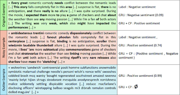
IMDb: The Fig. 5 displays a comparison of two texts before and after the random change of a few words (in bold) by other words in the model’s vocabulary. The actual text predicted as negative opinion by both models becomes positive for the GRU after disturbance. Nevertheless, the conformal model is more cautious by indicating that it can be both cases (). For the outlier example formed completely of vocabulary words, the GRU model predicts positive with a score of 0.99, while the conformal model says that it does not know ().

Fig. 5.

Examples of outlier and noisy texts compared to the original one for IMDb.

EGSS: The Fig. 6 displays a comparison of the positions of the test examples on the density regions before (a) and after (b) the addition of a Gaussian noise. This shows that several examples are positioned outside the density regions after the introduction of the disturbances. The outlier examples (c) created by modifying some characteristics of these test examples with extreme values (to simulate a sensor failure, for example) are even further away from the density regions, and recognized as such by the conformal model ().

Fig. 6.

Density visualization of real, noisy and outlier examples for EGSS.

Conclusions and Perspectives

We used the conformal prediction and the technique presented in [6] to have a more reliable and cautious deep learning model. The results show the interest of this method on different data types (image, text, tabular) used with different deep learning architectures (CNN, GRU and MLP). Indeed, in these three cases, the conformal model not only adds reliability and robustness to the deep model by detecting ambiguous examples but also keeps or even improves the performance of the basic deep model when it predicts only one class. We also illustrated the ability of conformal prediction to handle noisy and outlier examples for all three types of data. These experiments show that the conformal method can give more robustness and reliability to predictions on several types of data and basic deep architectures.

To improve the experiments and results, the perspectives include the optimization of density estimation based on neural networks. For instance, at a fixed the problem of finding the most efficient model arises that could be done by modifying the density estimation technique, but also by proposing an end-to-end, integrated estimation method. Also, it would be useful to compare the conformal prediction with calibration methods, for example, evidential ones that are also adopted for cautious predictions [3].

A Appendix

This appendix is to prove that Eqs. (9) and (10) in Sect. 2.3 are equivalent. We recall that Eq. (10) is

11

We recall that Eq. (9) uses the “greater or equal” sign. Here we need to use the “greater” signs in Eqs. (12) and (13) to have an equivalence, which is

12

such that

13

Let f(t) be the decreasing function .

Let us prove that (12) (11).

Since is the upper bound such that , then does not satisfy this inequality, thus

14

Since is a conformity score, whereas is a non-conformity score, we can write [14]. So (14) becomes

This shows that (12) (11).

Let us now prove that (11) (12). Using the indicator function of the complement, and changing the non-conformity score into a conformity score as shown before, we can simply find that

Using the same function f, we then have

15

Let us show by contradiction that . Suppose that . Since f is a decreasing function, we have . By the definition of , we have . Thus . However, this contradicts (15). So we proved that (11) (12), which concludes the proof.

References

- 1.Arzamasov, V.: UCI electrical grid stability simulated data set (2018). https://archive.ics.uci.edu/ml/datasets/Electrical+Grid+Stability+Simulated+Data+
- 2.Deng, J., Dong, W., Socher, R., Li, L.J., Li, K., Fei-Fei, L.: ImageNet: a large-scale hierarchical image database. In: CVPR (2009)
- 3.Denoeux T. Logistic regression, neural networks and Dempster-Shafer theory: a new perspective. Knowl.-Based Syst. 2019;176:54–67. doi: 10.1016/j.knosys.2019.03.030. [DOI] [Google Scholar]
- 4.Goodfellow, I.J., Shlens, J., Szegedy, C.: Explaining and harnessing adversarial examples. In: 3rd International Conference on Learning Representations, ICLR 2015, San Diego, CA, USA, 7–9 May 2015, Conference Track Proceedings (2015). http://arxiv.org/abs/1412.6572
- 5.He, K., Zhang, X., Ren, S., Sun, J.: Deep residual learning for image recognition. In: CVPR, pp. 770–778 (2016)
- 6.Hechtlinger, Y., Póczos, B., Wasserman, L.: Cautious deep learning. arXiv preprint arXiv:1805.09460 (2018)
- 7.Lei J, Robins J, Wasserman L. Distribution-free prediction sets. J. Am. Stat. Assoc. 2013;108(501):278–287. doi: 10.1080/01621459.2012.751873. [DOI] [PMC free article] [PubMed] [Google Scholar]
- 8.Liu, Z., Luo, P., Wang, X., Tang, X.: Deep learning face attributes in the wild. In: Proceedings of International Conference on Computer Vision (ICCV), December 2015
- 9.Maas, A.L., Daly, R.E., Pham, P.T., Huang, D., Ng, A.Y., Potts, C.: Learning word vectors for sentiment analysis. In: Proceedings of the 49th Annual Meeting of the Association for Computational Linguistics: Human Language Technologies, vol. 1, pp. 142–150 (2011)
- 10.Melluish T, Saunders C, Nouretdinov I, Vovk V. Comparing the Bayes and typicalness frameworks. In: De Raedt L, Flach P, editors. Machine Learning: ECML 2001; Heidelberg: Springer; 2001. pp. 360–371. [Google Scholar]
- 11.Papadopoulos, H.: Inductive conformal prediction: theory and application to neural networks. In: Tools in Artificial Intelligence. IntechOpen (2008)
- 12.Pedregosa F, et al. Scikit-learn: machine learning in python. J. Mach. Learn. Res. 2011;12:2825–2830. [Google Scholar]
- 13.Proedrou K, Nouretdinov I, Vovk V, Gammerman A. Transductive confidence machines for pattern recognition. In: Elomaa T, Mannila H, Toivonen H, editors. Machine Learning: ECML 2002; Heidelberg: Springer; 2002. pp. 381–390. [Google Scholar]
- 14.Vovk, V., Gammerman, A., Shafer, G.: Algorithmic Learning in a Random World. Springer, Heidelberg (2005). 10.1007/b106715