

Abstract
The measurement of polarization has been studied over the last thirty years. Despite the different applied approaches, since polarization concept is complex, we find a lack of consensus about how it should be measured. This paper proposes a new approach to the measurement of the polarization phenomenon based on fuzzy set. Fuzzy approach provides a new perspective whose elements admit degrees of membership. Since reality is not black and white, a polarization measure should include this key characteristic. For this purpose we analyze polarization metric properties and develop a new risk of polarization measure using aggregation operators and overlapping functions. We simulate a sample of  cases across a 5-likert-scale with different distributions to test our measure. Other polarization measures were applied to compare situations where fuzzy set approach offers different results, where membership functions have proved to play an essential role in the measurement. Finally, we want to highlight the new and potential contribution of fuzzy set approach to the polarization measurement which opens a new field to research on.
Keywords: Polarization, Fuzzy set, Ordinal variation
Introduction
Polarization is one of the most studied concepts in social sciences, specially over the last few years due to the recent growth of polarization episodes in different scenarios. The concept of polarization has been studied in social sciences from different perspectives [1, 6, 14, 16–18]. As can be seen after a fast literature review there is not an universal and accepted measure. As a consequence, there is not a well-defined consensus in the literature about what is the true nature of polarization.
Nevertheless, one of the most cited and used polarization measures was defined in the economics framework. Wolfson (1992) and Esteban and Ray (1994) among others, were some of the first authors in measuring polarization [5–7, 19]. These polarization measures are strongly linked to the concept of inequality. Since then, a growing number of diverse polarization measures has arisen, most of them based on the idea given in [6] and [7], although there are others that have also had a significant impact [1, 4, 16, 17].
It is important to remark that in the classical definition of Esteban and Ray of 1994 (and any other polarization measure based on Esteban and Ray) concepts like identification, membership, alienation and at the end aggregation are included in respective formulas.
Some of the previous concepts allow graduation and are vague in nature. For example, the way in which an individual feels identified with a group can be modeled by a fuzzy membership function. These functions represents the individual’s membership degree in a given group.
Focusing in the idea of Esteban and Ray in the bipolar case (i.e there are two extreme situations), in this paper we propose a new polarization measure expressed in terms of fuzzy membership functions. These functions are aggregated by adequate aggregation operators to obtain a final polarization score.
Preliminaries
Polarization Measures
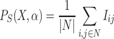
Polarization literature is essentially divided in two main approaches. First, those measures which only admit the existence of two groups, where the maximum polarization values are found in those cases where the group size is equal. According to this point of view, polarization follows a bimodal distribution (e.g.: Reynal-Querol, 2001 [17]). Otherwise, there are approaches which accept the presence of multiple groups. So that, those measures which take into account such diversity, are closer to terms like dispersion and variation. Since the more different values the more polarized is a population, the measure is moderated by the existence of two main groups with significant size. In this section, we focus our attention in measures based on diversity. Furthermore, we use the IOV index [2] as a reference measure in following sections because of its closeness to the concept of polarization.
-
Esteban and Ray (1994): Being one of the first polarization measures proposed, in [6] it is defined the ER polarization measure. This measure was proposed because of the need of measuring the polarization concept, where inequality indices do not fit to this task. Esteban and Ray aimed to establish a difference between polarization and inequality proposing three main basics of a polarization measure. So that, must be:
- a) high degree of homogeneity within groups.
- b) high degree of heterogeneity between groups.
- c) few number of groups with significant size.
To assess this, given a population of N individuals that take values X along a given numeric variable, in [6] the measurement of polarization is based on the effective antagonism approach. This is also called the IA approach that contains two concepts: identification (I) and alienation (a). The first one, reflects the degree in which a given individual feels closeness with the group that he/she belongs to. Otherwise, a shows the absolute distance between two individuals in terms of income.
Finally, the authors proposed the next polarization measure:
Where identification (I) is a function which depends on
1  group’s relative size, alienation (a) reflects the absolute distance between the groups
  and
and  . Regarding these two key aspects, effective antagonism is the product between I and a. It is worth mentioning that in the following years other authors have adapted ER measure (i.e. [4, 15]). This model assume a symmetric alienation between individuals. Authors also established an asymmetric model in [6].According to Eq. (1), the most used and simplified version of this formula (that we have denoted as
 here) are reformulated for those cases in which the only information available about the population N is the variable
 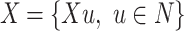 with its relative distribution:
  . So that, the following assumptions are made:
- The population N is partitioned into groups according to different values of X. An individual
 that takes the value
  belongs to the group
  .
. - The relative frequency of the group
 is denoted by
  .
. - The identification felt by one individual u to his/her group
 depend by the relative size of that group. In fact, we have that this value is
  . The value of
  should be greater than 1 (see [6]).
 - The value of
 that represents the discrepancy between these two groups (
 and
and  ) is the absolute difference between the values that they takes in the variable X, (i.e
  .
. - The alienation function a is the identification function.
- Finally, the function T is the product operator between the I and a.
Taking this into account, previous expression is commonly used as follow:
 |
2 |
Example 1
Let us have a given population N with  . Let the variable X be a variable that takes values
  with a relative frequency of 0.3, 0.5 and 0.2. Then:
 |
Let us recall again that the definition of Esteban and Ray of polarization (and of course its simplified version  ) assumes certain hypothesis that it is necessary to remark. From now on, we will denote by
  , the group that is denoted as
  by Esteban and Rey.
The different values of income present at X determine how many K groups are. So that, given a set of responses X with a finite domain
 , the class of groups
  are perfectly defined as
  .
.Individuals can be only assigned to one group, since the
 is a partition of N. Also let us observe that
- Given a group
 , if we denote
  as the degree to which the individual i feels identification to the group
  , this value is assumed to be:
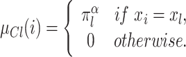
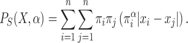
Taking previous considerations into account, formula (2) can be viewed as
 |
3 |
where  is the effective antagonism felt by person i to individual j that is not symmetric. The effective antagonism of two individuals is the aggregation T of two values: the identification of individual i with the group to which he/she belongs (
 ) and the alienation a of the discrepancy of the groups to which individuals i and j belong
  .
.
Example 2
Let 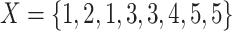 be a population of
  individuals. Following the assumptions of Esteban and Ray we have 5 groups that are perfectly identified with those individuals that takes values in
  . So the relative frequency are
  .
.
In order to obtain the final polarization score, we have to sum for each pair of relative frequencies the value  . Now we are going to see how this expression performs starting with two individuals i, j. Let us assume that
  and
and  . Then their values
  and
and  are 1 and 5 respectively. Assuming that
  ,
,  ,
,  we have that the expression corresponding to the individuals 1 and 7 is
 |
If we chose  for a clearer example, we have that
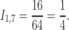
-
IOV Blair and Lacy. Ordinal index variation.
The concept of polarization have been confusing frequently with variation. Variability, dispersion and variance are key concepts in Statistics, and they are main argument to describe both the distribution of random variables and to describe the observed values of a statistical variable. In the last context, according to [12] the measurement of dispersion is usually associated to continuous statistical variables. When the dispersion has to be measured in ordinal variables (like for example a Likert-scale) the common approach is to convert the ordinal estimation into a numerical one by assigning numerical values to each ordinal variable category. Afterwards it is then possible to use a classical dispersion measure. But some authors [3, 8, 9] have pointed out that this procedure can lead to misunderstanding and misinterpretation of the measurement results.
Hence, some ordinal dispersion measures have been defined [3, 8, 9] to properly deal with ordinal statistical variables instead of forcing the use of classical measures (such as entropy, standard deviation, variance or quasivariance) that do take into account such ordinal characteristic.
Although other measures could be alternatively used within our ordinal framework, in this paper we will focus on the ordinal dispersion measure defined by Berry and Mielke [2], usually called as IOV.
Given an ordinal variable with values and a relative frequency vector
  , the ordinal dispersion measure IOV is defined as:
4
Aggregation Operators: Overlapping and Grouping Functions
Fuzzy set were introduced by Zadeh in 1965 [20], with the idea of sets with a continuum grades of membership, instead of the classical dual (yes/no) membership. Thus, as [13] remark in their work:
Definition 1
A fuzzy set  over the domain X is defined as
 |
where  represents a membership degree function, i.e.
  .
.
Aggregation Operators (AO) are one of the hottest disciplines in information sciences. AO appears in a natural way when the soft information has to be aggregated. At the beginning, AO were defined to aggregate values from membership functions associated to fuzzy set (see [20]). A key concept for the development of this paper is that of aggregation function.
Definition 2
A function  is said to be an n-ary aggregation function if the following conditions hold:
- (A1)
A is increasing in each argument: for each
 , if
, if  , then
  ;
;- (A2)
A satisfies the boundary conditions:
 and
and  .
.
It is important to emphasize that previous definition can be extended into a more general framework allowing to deal with more general objects than values into [0, 1].
Given two degrees of membership  and
and  of an object c into classes A and B, an overlap function is supposed to yield the degree z up to which the object c belongs to the intersection of both classes. Particularly, an overlap function was defined in [10] as a particular type of bivariate aggregation function characterized by a set of commutative, natural boundary and monotonicity properties. These authors extended the bivariate aggregation function to a n-dimensional case.
Definition 3
A function  is said to be an overlap function if the following conditions hold:
- (O1)
O is commutative;
- (O2)
 if and only if
  ;
;- (O3)
 if and only if
  ;
;- (O4)
O is increasing in each argument;
- (O5)
O is continuous.
Grouping functions are supposed to yield the degree z up to which the combination (grouping) of the two classes A and B is supported, that is, the degree up to which either A or B (or both) hold.
Definition 4
A function  is said to be a grouping function if the following conditions hold:
- (G1)
G is commutative;
- (G2)
 if and only if
  ;
;- (G3)
 if and only if
  or
or  ;
;- (G4)
G is increasing in each argument;
- (G5)
G is continuous.
Overlap functions are particularly useful. Furthermore, their applicability can be extended to community detection problems [11] or even to edge detection methods in the field of computer vision.
A New Polarization Measure from a Fuzzy Set Perspective: The One-Dimensional and Bipolar Case
In this section we are focused on the case in which the only available information of a given population is a one-dimensional variable X.
This variable X could be incomes (as it is assumed in ER approach) or even opinions. Now, let us assume that this variable X, presents two poles  and
and  . In this situation we will say that the variable X is bipolar or present two extreme values. Furthermore, we assume that the communication between individual for those extreme poles is broken, and thus, polarization does exist.
The only information we need to assume for the measure here propose is that we are able to measure the identification (or membership or closeness) of each individual with both extreme values/poles. Let us denote by  ,
,  the two membership degree functions that represent the membership degree.
  are functions and for each
  ,
,  and
and  represent the membership degree of individual i to the classes of extreme opinion
 and extreme opinion
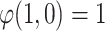
 respectively (Fig. 1).
Fig. 1.
A membership function of a bi-polarized population.
For this bipolar case, in which we assume the existence of two radical/extreme or poles opinions and we don’t have a-priori groups, we understand that polarization is associated when the following two situations appear:
a) A significant part of population is close to the pole
 .
.b) A significant part of population is close to the pole
 .
.
Also, as it happen with the ER case, we are going to assume that we are able to measure the discrepancy between these two poles or extreme situations by  .
.
Finally, the polarization measure that we propose here can be expressed as the sum of the aggregation of three important concepts and could be understood as the risk of polarization. Let us remark that polarization appears when two groups break their relationships and also their communication.
We consider the risk of polarization between two individuals (e.g.: i, j) as the possibility of these two situations:
How individual i is close to the extreme position
 and j is close to the other pole
  .
.How individual i is close to the extreme position
 and j is close to the other pole
  .
.
So that, if we assume that polarization appears in the last two situations we propose:
 |
5 |
where  is an overlapping aggregation operator and
  is a grouping function.
Example 3
To a better understand of the previous formula, let us analyze for a given pair of individuals  how the value is computed.
-
Case 1. Individual i is close to the pole A and j is close to the pole B. High polarization. In this case, we have that
 and
and  . Then we have to aggregate by a grouping function (
 ) two values: the degree to which i belong to A and j to B
  and the degree to which i belong to B and j to A
  .
.Finally, we have to verify which one of these two facts are true by a grouping function
 , since this is a case with high polarization.
 -
Case 2. Individuals i and j are in the middle of poles A and B. Here we propose the following case:
 and
and  . We have two individuals in the middle of the distribution. Then we have to aggregate by a grouping function the
  the results of two values: the degree to which i belong to A and j to B
  and the degree to which i belong to B and j to A
  .
.Finally, we have
 . Since this is a case with medium polarization.
 -
Case 3. Individual i is close to pole A and j is also close to pole B.
 and
and  . We have two individuals close to the pole A. No polarization case. Then we have to aggregate by a grouping function the
  the results of two value: the degree to which i belong to A and j to B
  and the degree to which i belong to B and j to A
  .
.Finally we have
 . Since this is a case with low polarization.
Remark 1
Also let us note that since  is an aggregation function, any increment of the three component will increase the polarization values for a fixed
  .
.
Remark 2
Those situations where a population X is partitioned into k groups, there will be as much groups as values are in the variable X (i.e.  ).
).
The previous bi-polarization index will be
 |
6 |
So that, the difference with the other polarization index is the way in which I(i, j) are measured for each pair of the groups  ,
,  .
.
A Comparison Between Polarization Measures in a 5-Liker Scale
Let us analyze the case in which we have a population with N individuals that takes values on a discrete/ordinal variable X with domain  . In order to build the JDJ polarization measure defined in the previous section, we need to chose the grouping, overlapping and membership functions that we are going to use. For simplicity, the grouping function that we have chosen is the Maximum aggregation operator. Furthermore, we are going to study two well-known overlapping functions: the minimum and the product. Finally we are going to analyze a triangular membership function
  (see Fig. 2):
 |
7 |
Fig. 2.

Membership degree  for the two extreme poles
  ,
,  .
.
It is possible to consider different triangular membership functions too. For example, we can reduce the triangular membership function domain if we want to force the  function to zero for those values in x greater than a as well as to force the
  function to be zero for those values in x lower than b.
For this experiment we have always considered  and
and  or
or  . We have also considered two options for JDJ polarization index denoted by
  and
and  .
.
In the following experiment, we reproduce a sample of  cases and their different relative frequency distributions along a 5-Likert Scale with the same probability.
Therefore, three polarization measures were applied and compared for each case: Esteban and Ray measure (ER), and the last two index mentioned above  (
( ) and
) and  (
( ). Furthermore, an index of ordinal variance (IOV) is applied. Thus, next table shows some descriptive statistics for the measures applied (Table 1).
Table 1.
Descriptive statistics for IOV, ER,  and
and  .
.
| Mean | SD | Median | Trimmed | Mad | Min | Max | Range | Skew | Kurtosis | |
|---|---|---|---|---|---|---|---|---|---|---|
| IOV | 0.60 | 0.17 | 0.60 | 0.60 | 0.19 | 0.00 | 1.00 | 1.00 | −0.15 | −0.49 |
| ER | 0.37 | 0.10 | 0.35 | 0.36 | 0.10 | 0.00 | 1.00 | 1.00 | 0.80 | 1.17 |
 |
0.75 | 0.13 | 0.76 | 0.76 | 0.12 | 0.00 | 1.00 | 1.00 | −0.85 | 1.23 |
 |
0.28 | 0.18 | 0.27 | 0.27 | 0.20 | 0.00 | 1.00 | 1.00 | 0.41 | −0.37 |
As the following histograms suggest (see Fig. 3), it is worth mentioning the opposite skewed between ER and  measures, finding lower ER values of polarization than
  . In fact, this is a key aspect between both measures that underlies a difference between their conceptual and model properties that we explain below. Otherwise, low values of polarization are shown by
  . It is due to the membership function of
  .
.
Fig. 3.
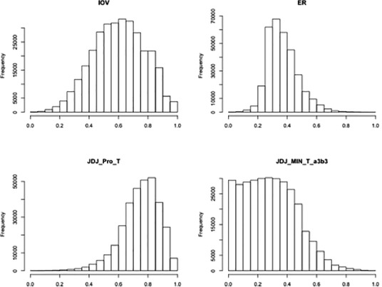
Underlying frequency distribution for IOV, ER,  and
and  .
.
In Fig. 4 we show the relationship between each polarization measure and the IOV values grouped by deciles. We can see a natural tendency to find the higher polarization the higher IOV values. In fact, correlation between IOV and all polarization measures can be found in the figure below, where  shows the highest correlation value (0.87),
  has a correlation value of 0.843 and ER shows the lower (0.78). Otherwise, we can see in ER measure a significant portion of medium values of polarization in the first decile of IOV, finding a lack of stability in this scenario.
Fig. 4.

Box plot displaying a distribution of polarization measures (ER,  and
and  ) for each decile of IOV.
Conclusions and Final Remarks
The concept of polarization is rich and complex and there is a need to find an approach which includes both metric and conceptual perspectives at the same time. According to this, for those cases where not all information are available in data (such as communication flow), we shall propose not to mean polarization itself but a risk of polarization for the bipolar case.
In this work, we present a fuzzy set approach to measure the risk of bi-polarization. Moreover, polarization has been understood as a synonym of variation. Regarding this, despite we find high correlation between ordinal variation and polarization values, we want to highlight that these small discrepancies make the difference.
Otherwise, as another main proposal in this work, is to provide a new methodology on the measurement of polarization. As a main tool to this new point of view, fuzzy set provides the appropriate resources. In one hand, in daily life people does not only feel identified with one single group but to some others too. Although, this duality is not a strict dichotomy but a long spectrum of nuances. Reality is fuzzy itself. As an example, an individual can be a strong supporter of a given political party but being identified with some contrary party proposals as well. In other hand, from a metric building perspective, using aggregation operators and membership functions, fuzzy set approach allows to pursue this philosophy. The membership functions used in this work are just a general example to apply this methodology. Along the different 391315 populations for a 5 likert scale, we have seen how the membership function determines the model behaviour. Specially for both measures proposed here, whose different membership functions reflect different results. Other membership functions more adequate are up to being develop for being applied.
Specifically, this key aspect has two main consequences: a) the frequency or bias to show high or low values of each polarization measure and b) those specific scenarios where high or low values should appear. It is important the equivalence between this membership functions and reality (e.g.: in those cases where individuals get clustered into two antagonistic groups, a given polarization measure should offer its highest values).
To conclude, we suggest for some directions for future research. Regarding membership functions, we consider as an important task to research about which membership function is more adequate for a given scenario. Furthermore, to develop new polarization measure incorporating a multi-dimensional case with multiples features. Moreover, including more theoretical polarization concepts like communication flow is needed to build an adequate polarization measure.
Footnotes
Supported by PGC2018-096509-B-I00 national project.
Contributor Information
Marie-Jeanne Lesot, Email: marie-jeanne.lesot@lip6.fr.
Susana Vieira, Email: susana.vieira@tecnico.ulisboa.pt.
Marek Z. Reformat, Email: marek.reformat@ualberta.ca
João Paulo Carvalho, Email: joao.carvalho@inesc-id.pt.
Anna Wilbik, Email: a.m.wilbik@tue.nl.
Bernadette Bouchon-Meunier, Email: bernadette.bouchon-meunier@lip6.fr.
Ronald R. Yager, Email: yager@panix.com
Juan Antonio Guevara, Email: juanguev@ucm.es.
Daniel Gómez, Email: dagomez@estad.ucm.es.
José Manuel Robles, Email: jmrobles@ccee.ucm.es.
Javier Montero, Email: monty@mat.ucm.es.
References
- 1.Apouey B. Measuring health polarization with self-assessed health data. Health Econ. 2007;16(9):875–894. doi: 10.1002/hec.1284. [DOI] [PubMed] [Google Scholar]
- 2.Berry KJ, Mielke PW., Jr Indices of ordinal variation. Percept. Mot. Skills. 1992;74(2):576–578. doi: 10.2466/pms.1992.74.2.576. [DOI] [Google Scholar]
- 3.Blair J, Lacy M. From the sage social science collections. Rights reserved. Sociol. Methods Res. 2000;28(3):251–280. doi: 10.1177/0049124100028003001. [DOI] [Google Scholar]
- 4.Duclos JY, Esteban J, Ray D. Polarization: concepts, measurement, estimation. Econometrica. 2004;72(6):1737–1772. doi: 10.1111/j.1468-0262.2004.00552.x. [DOI] [Google Scholar]
- 5.Esteban, J., Ray, D.: On the measurement of polarization, Boston university, institute for economic development, working paper 18 (1991)
- 6.Esteban JM, Ray D. On the measurement of polarization. Econ.: J. Econ. Soc. 1994;62(4):819–851. doi: 10.2307/2951734. [DOI] [Google Scholar]
- 7.Foster, J.E., Wolfson, M.C.: Polarization and the decline of the middle class: Canada and the US mimeo. Vanderbilt University (1992)
- 8.Franceschini F, Galetto M, Varetto M. Qualitative ordinal scales: the concept of ordinal range. Qual. Eng. 2004;16(4):515–524. doi: 10.1081/QEN-120038013. [DOI] [Google Scholar]
- 9.Gadrich T, Bashkansky E. Ordanova: Analysis of ordinal variation. J. Stat. Plan. Infer. 2012;142(12):3174–3188. doi: 10.1016/j.jspi.2012.06.004. [DOI] [Google Scholar]
- 10.Gómez D, Rodriguez JT, Montero J, Bustince H, Barrenechea E. n-dimensional overlap functions. Fuzzy Sets Syst. 2016;287:57–75. doi: 10.1016/j.fss.2014.11.023. [DOI] [Google Scholar]
- 11.Gomez D, Rodríguez JT, Yanez J, Montero J. A new modularity measure for fuzzy community detection problems based on overlap and grouping functions. Int. J. Approximate Reasoning. 2016;74:88–107. doi: 10.1016/j.ijar.2016.03.003. [DOI] [Google Scholar]
- 12.Martínez N, Gómez D, Olaso P, Rojas K, Montero J. A novel ordered weighted averaging weight determination based on ordinal dispersion. Int. J. Intell. Syst. 2019;34(9):2291–2315. doi: 10.1002/int.22168. [DOI] [Google Scholar]
- 13.Montero J, González-del Campo R, Garmendia L, Gómez D, Rodríguez JT. Computable aggregations. Inf. Sci. 2018;460:439–449. doi: 10.1016/j.ins.2017.10.012. [DOI] [Google Scholar]
- 14.Morales AJ, Borondo J, Losada JC, Benito RM. Measuring political polarization: Twitter shows the two sides of venezuela. Chaos: Interdiscip. J. Nonlinear Sci. 2015;25(3):033114. doi: 10.1063/1.4913758. [DOI] [PubMed] [Google Scholar]
- 15.Permanyer I, D’Ambrosio C. Measuring social polarization with ordinal and categorical data. J. Publ. Econ. Theory. 2015;17(3):311–327. doi: 10.1111/jpet.12093. [DOI] [Google Scholar]
- 16.Permanyer I. The conceptualization and measurement of social polarization. J. Econ. Inequality. 2012;10(1):45–74. doi: 10.1007/s10888-010-9143-2. [DOI] [Google Scholar]
- 17.Reynal-Querol, M.: Ethnic and religious conflicts, political systems and growth. Ph.D. thesis, London School of Economics and Political Science (University of London) (2001)
- 18.Wang YQ, Tsui KY. Polarization orderings and new classes of polarization indices. J. Publ. Econ. Theory. 2000;2(3):349–363. doi: 10.1111/1097-3923.00042. [DOI] [Google Scholar]
- 19.Wolfson MC. When inequalities diverge. Am. Econ. Rev. 1994;84(2):353–358. [Google Scholar]
- 20.Zadeh LA. Fuzzy sets. Inf. control. 1965;8(3):338–353. doi: 10.1016/S0019-9958(65)90241-X. [DOI] [Google Scholar]