Fuzzy Set Based Models Comparative Study for the TD TSP with Rush Hours and Traffic Regions

Abstract

This study compares three fuzzy based model approaches for solving a realistic extension of the Time Dependent Traveling Salesman Problem. First, the triple Fuzzy (3FTD TSP) model, where the uncertain costs between the nodes depend on time are expressed by fuzzy sets. Second, the intuitionistic fuzzy (IFTD TSP) approach, where including hesitation was suitable for quantifying the jam regions and the bimodal rush hour periods during the day. Third, the interval-valued intuitionistic fuzzy sets model, that calculates the interval-valued intuitionistic fuzzy weighted arithmetic average (IIFWAA) of the edges’ confirmability degrees and non-confirmability degrees, was contributing in minimizing the information loss in cost (delay) calculation between nodes.

Introduction

The Traveling Salesman Problem (TSP) is one of the extensively studied NP-hard graph search problems [1]. Various approaches are known for finding the optimum or semi optimum solution. The Time Dependent Traveling Salesman Problem (TD TSP) is a more realistic extension of the TSP, where the costs of edges vary in time, depending on the jam regions and rush hours. In the TD TSP, the edges are assigned higher weights if they are traveled within the traffic jam regions during rush hour periods, and lower weights otherwise [2]. The information on the rush hour periods and jam regions is uncertain and vague (fuzzy), hence, representing them by crisp numbers in the classic TD TSP does not quantify the effects of traffic jams accurately [2]. This limitation of simulating real life cases was to the point in constructing three novel fuzzy models capable of addressing the TD TSP with jam regions and rush hours more efficiently. In the Triple Fuzzy (3FTD TSP) model, the costs between the nodes may depend on time and location; and are expressed by fuzzy sets [3]. Here, fuzzy values represent the uncertainties of the costs caused by the fuzzy extensions of the traffic jam areas and rush hour times, which depend on several vague or non-deterministic factors. Rush hour time was represented as a bimodal piecewise linear normal fuzzy set, the jam areas as fuzzy oblongs, and the costs as trapezoidal sets. This model expressed the uncertain costs affected by the jam situations, and calculated the overall tour length quantitatively [3]. Second, the Intuitionistic Fuzzy IFTD TSP approach, involves a hesitation part expressing the effects of membership and non-membership values allowing a higher level of uncertainty [4]. In the IFTD TSP, the use of intuitionistic fuzzy sets ensured an even more realistic cost estimate of the TD TSP problem. By successfully representing simultaneously the higher degrees of association and the lower degrees of non-association of the jam factor and rush hours and lower degrees of hesitation to edges cost, resulted in a more accurate cost of the tours [4]. Third, we proposed the interval-valued intuitionistic fuzzy set model (IVIFTD TSP) [5]. In the IVIFTD TSP, additional uncertainty was modeled, and by using an aggregation of the costs rather than using the max-min composition of the fuzzy factors resulted in an even more adequate model. In this paper, the three models are briefly presented and examined, from the point of view of realistical representation and results.

Solution of the Classic TSP

The original TSP was first formulated in 1930 [6]. A salesman starts the journey from the headquarters and visits each city or shop exactly once then returns to the starting point. The task is to find the route with minimum overall travelled distance visiting all destination points. TSP is a graph search problem with edge weights in Eq. 1. In the symmetric case with n nodes c_ij = c_ji, so, in the graph, there is only one edge between every two nodes. Let x_ij = {0, 1} be the decision variable (i, j = 1, 2, …, n), and x_ij = 1, if edge e_ij between node_i and node_j is part of the tour. Let , , C is called cost matrix, where C_ij represent the cost of going from city i to city j. then:

1

2

The goal is to find the directed Hamiltonian cycle with minimal total length.

The Time Dependent TSP (TD TSP)

Despite TD TSP’s good results in determining the overall cost for a trip under realistic traffic conditions, yet one major drawback is the crisp values used for the proportional jam factors [2]. The total cost of any trip consists of two main elements: costs proportional to physical distances and costs increased by traffic jams occurring in rush hour periods or in certain areas between the pairs of nodes (such as in city center areas). The first can be looked at as constant; although transit times are subject to external and unexpected environmental factors. Thus, even they should be treated as uncertain variables, in particular, as fuzzy cost coefficients. In the TD TSP, the edges have fixed costs, which may be multiplied by a rush hour factor). This representation of the traffic jam effects is too rigid for real life circumstances.

The Triple Fuzzy TD TSP (3FTD TSP)

In the 3FTD TSP approach [Put here a citation of our paper] two parameters modify the fuzzy edge costs, the actual jam factor calculated from the membership degree of being in the jam region, and the degree of membership being in the rush hour period in the given moment. We proposed to use a simple Mamdani rule base [7] in the form: If is in the traffic jam region J and is in the rush hour time R then the cost is . Here, membership functions from the unit interval [0, 1] help describe the uncertainty of the jam region and the rush hour period, more efficiently. In this model, the distance between cities is also expressed in terms of the elapsed time. Here, we introduced a velocity (v) as a new parameter of the TSP route. The costs were represented by asymmetrical triangular fuzzy numbers. The total cost of the tour was calculated as follows:

3

where and are obtained from the Fuzzy Jam Region (J) and Fuzzy Traffic Rush Hours (R) membership functions. A valid solution for the problem is a permutation of the nodes:

4

where is the starting and end node of the tour. The time needed for visiting the first city from the start node is:

5

where P₁ is the starting node, P₂ is the first visited one and v is the velocity. The calculation of travel time is necessary as the costs are time dependent, and the actual cost between two cities can be determined by Eq. 3, thus, the time dependency in the cost matrix is represented by virtual distance values. The cost of the trip is calculated from

6

The total cost is:

7

where is the location last visited, and is the total time elapsed from the beginning of the tour till the salesman arrives in city . In the implementation, the three fuzzy elements used were triangular fuzzy costs between the edges, fuzzy oblong type membership function(s) of the fuzzy jam region(s) J; and bimodal normal piecewise linear membership function(s) for the traffic rush hour time period(s) R – see next sections.

Triangular Fuzzy Costs for the “Distances”

The uncertain costs between the nodes, is expressed by triangular fuzzy numbers. Triangular fuzzy numbers may be expressed by the support C = [C_L, C_R], and the peak value C_C is, so it is denoted by  = (C_L, C_C, C_R). To calculate the overall distance of the tour, these fuzzy values are summed up. The calculation of the total length of the tour was done by the defuzzified values of the fuzzy numbers using Center of Gravity (COG) [8].

The Membership Function of the Jam Regions

The fuzzy extensions of the city center areas (the degree of belonging to the jam region J) are expressed by fuzzy borders as in Fig. 1. Thus, μ₁ is simply calculated as , where d1, d2 are the distances from the peak of J. This approach sophisticates Schneider’s original model (cf. [2]), so that the breakpoints are: [0, 1000, 5000, 6000], (see Fig. 1).

Fig. 1.

Jam regions membership function (J)

Membership Function of the Traffic Rush Hour Periods

The model uses the bimodal membership function in Fig. 2 for representing the Traffic Rush Hour Time (). In this example, the two peak rush hour periods are from 7 to 8 a.m. and from 4 to 6 p.m. Between the two periods the traffic is lower. (We used the traffic data base …). The breakpoints of J are {0, 5, 7, 8, 14, 16, 18, 22, 24}, and its membership value at 14 h is 0.75. For illustration, assuming a jam factor of 5, a sample calculation is run to clarify the approach. The peak point of the fuzzy triangular cost for each edge is the Euclidean distance between the end-points, namely, the left-side and right-side points were determined randomly (0–50% lower and higher than the middle point) in this test.

Fig. 2.

Rush hours membership function (R)

Table 1 was calculated by averaging five times runs for jam factor 5.0 for the three areas of the triangular membership functions (low, medium and high). Table 2 shows the middle values of the supports of the triangular fuzzy numbers for that specific case (for jam factor 5). Depending on Table 1 the average elapsed time is 22.19562.

Table 1.

Computational results for jam factor equal 5.0.

	Run 1	Run 2	Run 3	Run 4	Run 5
Elapsed time	22.2021	22.1314	22.3246	22.3067	22.0133
Low	16.5611	16.2926	16.5862	16.642	16.8112
Middle	22.4831	22.6905	22.4858	23.0948	22.3641
High	27.562	27.4111	27.9018	27.2832	27.3146

Table 2.

Support value for jam factor 5

Run 1	Run 2	Run 3	Run 4	Run 5	Average elapsed time
11.0009	11.1185	11.3156	10.6412	10.5034	10.91592

Applying the same approach results in Table 3, which contains the total time in hours required to visit each location with different jam factors by applying the same concept explained in the previous section

Table 3.

Computational results for the 3FTD TSP.

Jam factor	Average elapsed time
1.00	19.5
1.05	19.6
1.20	19.7
1.50	20.3
2.00	20.9
3.00	21.6
5.00	22.2
10.00	23.1
20.00	23.5
50.00	24.2
100.00	24.7

With such high jam factors, the tour lengths were longer for the 3FTD TSP problem, because the traffic jam period is longer compared to the classic TD TSP.

Intuitionistic Fuzzy TD TSP (IFTD TSP)

In this model, we moved one step further and extended the model by using intuitionistic fuzzy set theory. First some related definitions as introduced [4].

Basic Definitions of Intuitionistic Fuzzy Sets (IFS)

Let a universal set E be fixed and . An intuitionistic fuzzy set or IFS A in E is an object having the form

8

The amount is called the hesitation part, which may cater to either the membership value or to the non-membership value, or to both [9, 10]. If A is an IFS of X, the max-min-max composition of the If Relation (IFR) R (X → Y) with A is an IFS B of Y denoted by and is defined by the membership function

9

and the non-membership function

10

The previous formulas hold for all Y. Let and be two IFRs. The max-min-max composition is the intuitionistic fuzzy relation from X to Z, defined by the membership function

11

and the non-membership function is given by

12

Let A be an IFS of the set J, and R be an IFR from J to C. Then the max-min-max composition B of IFS A with the IFR R () denoted by gives the cost of the edges as an IFS B of C with the membership function given by

13

and the non-membership function given as:

14

If the state of the edge E is described in terms of an IFS A of J; then E is assumed to be the assigned cost in terms of IFSs B of C, through an IFR R from J to C, which is assumed to be given by a knowledge base directory (given by experts) on the destination cities and the extent (membership) to which each one is included in the jam region. This will be translated to the degrees of association and non-association, respectively, between jam and cost.

IFTD TSP Applied on the TD TSP Case

Let there be n edges E_i; i = 1; 2;…, 16 as in Fig. 3; in a trip. Thus . Let R be an IFR and construct an IFR Q from the set of edges E to the set of jam factors J. Clearly, the composition T of IFRs R and give the cost for each edge from E to C by the membership function given as:

15

and the non-membership function given as:

16

Fig. 3.

Tour for a simple example

For given R and Q, the relation can be computed. From the knowledge of Q and T, an improved version of the IFR R can be computed, for which the following holds valid:

• (i) is greatest
• (ii)The equality is retained

Table 4 shows each edge of the tour and the jam factors associated. The ultimate goal is to be able to calculate the total tour jam factor which will be multiplied by the physical distances between two nodes. The intuitionistic fuzzy relations are given as shown in Table 4, and as in Table 5, and the composition as in Table 6. Then we calculated the jam region cost factors (see Table 7), where the four cost factors are with weighted average calculations:

17

Table 4.

Route1 = (Edge 1 … Edge 17)

(Q)	Jam Region1	Jam Region2	Jam Region3	Jam Region4
E1	(0.8, 0.1)	(0.6, 0.1)	(0, 1)	(0, 1)
E2	(0, 1)	(0, 1)	(0.2, 0.8)	(0.6, 0.1)
E3	(0.8, 0.1)	(0.8, 0.1)	(0, 1)	(0, 1)
E4	(0, 1)	(0, 1)	(0, 0.6)	(0.2, 0.7)
E5	(0.8, 0.1)	(0.8, 0.1)	(0, 0.6)	(0.2, 0.7)
E6	(0, 0.8)	(0.4, 0.4)	(0, 1)	(0, 1)
E7	(0, 1)	(0, 1)	(0.6, 0.1)	(0.1, 0.7)
E8	(0, 0.8)	(0.4, 0.4)	(0.6, 0.1)	(0.1, 0.7)
E9	(0.6, 0.1)	(0.5, 0.4)	(0, 1)	(0, 1)
E10	(0, 1)	(0, 1)	(0.3, 0.4)	(0.7, 0.2)
E11	(0, 0.8)	(0.4, 0.4)	(0.6, 0.1)	(0.1, 0.7)
E12	(0, 0.8)	(0.4, 0.4)	(0, 1)	(0, 1)
E13	(0, 1)	(0, 1)	(0.2, 0.8)	(0.6, 0.1)
E14	(0, 1)	(0, 1)	(0.6, 0.1)	(0.1, 0.7)
E15	(0.8, 0.1)	(0.8, 0.1)	(0, 0.6)	(0.2, 0.7)
E16	(0, 0.8)	(0.4, 0.4)	(0.6, 0.1)	(0.1, 0.7)
E17	(0.6, 0.1)	(0.5, 0.4)	(0, 1)	(0, 1)

Table 5.

Jam factors

Jam area (R)	Cost factor 1 (c1)	Cost factor 2 (c2)	Cost factor 3 (c3)	Cost factor 4 (c4)
Jam Region1	(0.4, 0)	(0.7, 0)	(0.3, 0.3)	(0.1, 0.7)
Jam Region2	(0.3, 0.5)	(0.2, 0.6)	(0.6, 0.1)	(0.2, 0.4)
Jam Region3	(0.1, 0.7)	(0, 0.9)	(0.2, 0.7)	(0.8, 0)
Jam Region4	(0.4, 0.3)	(0.4, 0.3)	(0.2, 0.6)	(0.2, 0.7)

Table 6.

Jam cost (T)	Cost factor 1	Cost factor 2	Cost factor 3	Cost factor 4
E1	(0.4, 0.1)	(0.7, 0.1)	(0.6, 0.1)	(0.2, 0.4)
E2	(0.4, 0.3)	(0.4, 0.3)	(0.2, 0.6)	(0.2, 0.2)
E3	(0.4, 0.1)	(0.7, 0.1)	(0.6, 0.1)	(0.2, 0.4)
E4	(0.2, 0.7)	(0.2, 0.7)	(0.2, 0.7)	(0.2, 0.6)
E5	(0.3, 0.1)	(0.7, 0.1)	(0.6, 0.1)	(0.2, 0)
E6	(0.3, 0.5)	(0.2, 0.6)	(0.4, 0.4)	(0.2, 0.4)
E7	(0.1, 0.7)	(0.1, 0.7)	(0.2, 0.7)	(0.6, 0.1)
E8	(0.3, 0.5)	(0.2, 0.6)	(0.4, 0.4)	(0.6, 0.1)
E9	(0.4, 0.1)	(0.6, 0.1)	(0.5, 0.3)	(0.2, 0.4)
E10	(0.4, 0.3)	(0.2, 0.6)	(0.2, 0.6)	(0.3, 0.4)
E11	(0.3, 0.5)	(0.2, 0.6)	(0.4, 0.4)	(0.6, 0.1)
E12	(0.3, 0.5)	(0.2, 0.6)	(0.4, 0.4)	(0.2, 0.4)
E13	(0.4, 0.3)	(0.4, 0.3)	(0.2, 0.6)	(0.2, 0.2)
E14	(0.1, 0.7)	(0.1, 0.7)	(0.2, 0.7)	(0.6, 0.1)
E15	(0.3, 0.1)	(0.7, 0.1)	(0.6, 0.1)	(0.2, 0)
E16	(0.3, 0.5)	(0.2, 0.6)	(0.4, 0.4)	(0.6, 0.1)
E17	(0.4, 0.1)	(0.6, 0.1)	(0.5, 0.3)	(0.2, 0.4)

Table 7.

Intuitionistic jam region costs for edges

JR	JR1	C1	JR2	C2	JR3	C3	JR4	C4	Total jam regions cost
E1	0.35	1.2	0.68	1.5	0.57	2	0.04	5	1.695
E2	0.31	1.2	0.31	1.5	0.08	2	0.08	5	1.791
E3	0.35	1.2	0.68	1.5	0.57	2	0.04	5	1.695
E4	0.13	1.2	0.13	1.5	0.13	2	0.08	5	2.151
E5	0.24	1.2	0.68	1.5	0.57	2	0.2	5	2.04
E6	0.2	1.2	0.08	1.5	0.32	2	0.36	5	2.97
E7	0	1.2	0	1.5	0.13	2	0	5	2
E8	0.2	1.2	0.08	1.5	0.32	2	0.57	5	3.291
E9	0.35	1.2	0.57	1.5	0.44	2	0.04	5	1.682
E10	0.31	1.2	0.08	1.5	0.08	2	0.18	5	2.388
E11	0.2	1.2	0.08	1.5	0.32	2	0.57	5	3.291
E12	0.2	1.2	0.08	1.5	0.32	2	0.36	5	2.917
E13	0.31	1.2	0.31	1.5	0.08	2	0.08	5	1.791
E14	0	1.2	0	1.5	0.13	2	0	5	2
E15	0.24	1.2	0.68	1.5	0.57	2	0.2	5	2.04
E16	0.2	1.2	0.08	1.5	0.32	2	0.57	5	3.291
E17	0.35	1.2	0.57	1.5	0.44	2	0.04	5	1.682

The rush hour cost factors of each tour edge are determined in a similar intuitionistic model. The relations between the tour time and the rush hour periods () are described with intuitionistic fuzzy functions in Fig. 4. An IFR () is given between the rush hour periods and the cost factors similarly, as it was done for the jam regions in Table 5. Then the composition is calculated. Finally, rush hour cost factors were calculated with weighted averaging. The cost of the edges is calculated taking into account the two cost factors ( is the Euclidean distance):

Fig. 4.

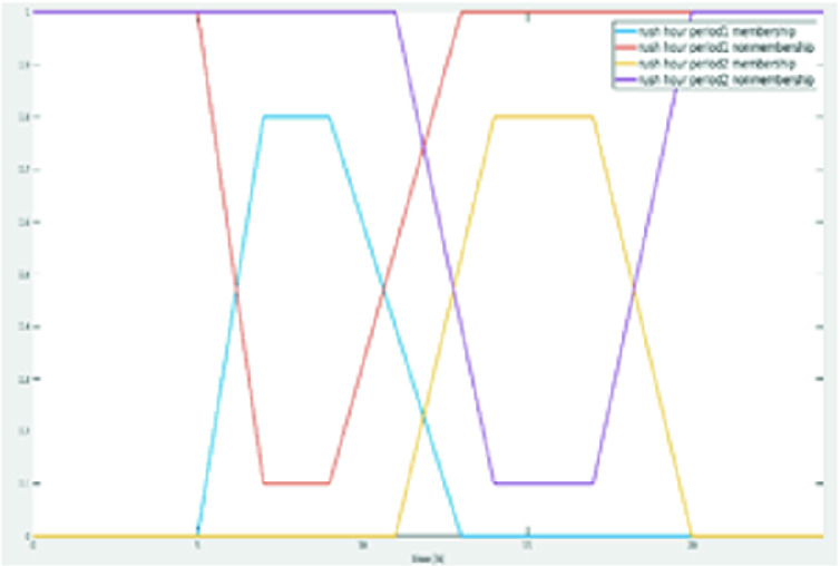
Fuzzy membership and non- membership functions of the rush hour periods

IF AND [the edge belongs to at least one of the jam regions and is passed during rush hour periods] THEN ELSE .

Clearly, the improved version of R in the IFTD TSP model is more adequate in translating the higher degrees of association and lower degrees of non-association of the jam factors and rush hours as well as lower degrees of hesitation to any cost C; If almost equal values in T are obtained, then we consider the case for which hesitation is least. From a refined version of R one may infer cost from jam factors in the sense of a paired value, one being the degree of association and other the degree of non-association. Ultimately, this model offers more realistic costs calculation for the traveled routes under real traffic conditions.

The Interval Valued IFTD TSP (IVIFTD TSP)

First, some basic definitions are overviewed [11, 12]. In a type-2 fuzzy set, the uncertain values of the membership function in Eq. 18 consists of a rounded region called “footprint of uncertainty” (FOU). It is the union of all primary memberships

18

FOUs emphasize the distribution that sits on top of the primary membership function of the type-2 fuzzy set. The shape of this distribution depends on the choice made for the secondary grades. When they are equal between two bounds, it gives an interval type-2 fuzzy set as given in Eq. 19.

19

For discrete universe of discourse , an embedded type-2 set has elements, where contains exactly one element from set , namely , with its associated secondary grade , , which equals to Eq. 20.

20

As we discussed previously, the jam factor costs on the edges in a tour were represented as fuzzy relations between the jam factors and the predicted costs (delays).

Let , and denote the sets of jam factors, costs and edges, respectively. Two fuzzy relations (FR) Q and R are defined in Eqs. 21 and 22.

21

22

where and indicates jam factors degrees for edges. The degree is the relationship between the edges and the jam factors (rush hours or jam regions). Hence, indicates the degree to which jam factor j affects edge E and indicates the degree to which jam factor j does not affect the same edge. Similarly, and are the relationships between the jam factors and the respective costs. (This is called confirmability degree in the coming sections). represents the degree to which jam factor j confirms, and the degree to which jam factor j does not confirm the presence of cost c, respectively [5]. Since Q is defined on set and R on set the composition T of R and Q () for the prediction of the cost for a specific edge in terms of the cost can be represented by FR from E to C, given the membership function in Eq. 23 and non membership function in Eq. 24 for all

23

24

Let any two IVIFS be a collection of interval-valued intuitionistic fuzzy degrees. Then, an IIFWAA operator is defined in Eq. (25)

25

In the next section, we explain the IVIFTD TSP by simulating a simple real life TD TSP cost problem. The approach consists of four main steps:

Step 1. Prediction for the rush hours and jam regions of the edges, in the sense that if the trip between the two cities happens during the rush hours and within the jam regions, both will be taken into consideration and none of the factors will be neglected. Table 8 identifies the cost of each jam factor, which is supposed to be predefined by experts in this domain, according to the rush hours and the jam regions.

Table 8.

Knowledge base for rush hours and jam regions costs

Traffic factor	IF degree
	Cost1		Cost2		Cost3
Factor 1.1	[0.6, 0.7]	[0.1, 0.2]	[0.2, 0.3]	[0.5, 0.6]	[0.1, 0.3]	[0.4, 0.6]
Factor 1.2	[0.6, 0.7]	[0.2, 0.3]	[0.2, 0.4]	[0.4, 0.6]	[0.4, 0.6]	[0.1, 0.2]
Factor 1.3	[0.5, 0.6]	[0.1, 0.2]	[0.1, 0.2]	[0.6, 0.7]	[0.3, 0.4]	[0.3, 0.5]
Factor 1.4	[0.7, 0.8]	[0.1, 0.2]	[0.1, 0.2]	[0.6, 0.8]	[0.1, 0.2]	[0.7, 0.8]
…	…	…	…	…	…	…
Factor 2.1	[0.5, 0.6]	[0.2, 0.3]	[0.2, 0.3]	[0.4, 0.6]	[0.2, 0.3]	[0.5, 0.6]
Factor 2.2	[0.7, 0.8]	[0.1, 0.2]	[0.1, 0.2]	[0.6, 0.7]	[0.1, 0.2]	[0.6, 0.7]
…	…	…	…	…	…	…
Factor n.1	[0.6, 0.8]	[0.1, 0.2]	[0.1, 0.2]	[0.6, 0.7]	[0.2, 0.3]	[0.6, 0.7]
Factor n.n

Step 2. Calculation of the interval-valued intuitionistic fuzzy weighted arithmetic average (IIFWAA) of the edges’ confirmability and non-confirmability degrees, respectively with the chosen aggregation [13]. where are the weight vectors of A. Further, . In our model we propose giving equal weights to the factors by . For finding the final jam factor cost, we first calculate the IIFWAA from the degrees given in Table 8 and then use a measure based on distance between IVIFS.

Step 3. Calculating the distance between the IFSs using the IIFWAA obtained in Step 2.

To calculate the jam factor cost based on the Park distance model between IVIFS [14]. Particularly, we consider the hesitation part to modify the Park distances. The normalized Hamming distance considering the hesitation part, is defined as below for any and ). The normalized Hamming distance considering the hesitation part (where H is the hesitation part) is defined as:

26

Step 4. Determination of the final jam factor affected costs based on the distance (assuming equal weights for all factors).

The IVIFTD TSP Model Applied on the TD TSP Case

To illustrate how to apply the proposed new model on a TD TSP case study with double uncertain jam regions and rush hours, let us consider that E1 is the first edge of a tour as in Fig. 4. There are different traffic factors assumed, they may represent jam regions or rush hours Factors (1.1, 1.2, 1.3, 1.4, 2.1 and 2.2 in bold Table 8) affecting E1 simultaneously. Here, we use assigned by domain experts, to indicate the degrees how a jam factor j affects edge e as in Eq. 23, and the confirmability degree as in Eq. 24 is given by .

Step 1. Table 9 shows the confirmability and non-confirmability degrees of the jam factors assigned to E1, according to their degree of belonging to the rush hour periods and jam regions

Table 9.

E1 degrees of jam factors. ,

E1 traffic factors	1.1	1.2	1.3	1.4	2.1	2.2
	[0.5, 0.6]	[0.5, 0.6]	[0.4, 0.6]	[0.7, 0.8]	[0.5, 0.6]	[0.5, 0.7]
	[0.2, 0.3]	[0.1, 0.3]	[0.1, 0.2]	[0.1, 0.2]	[0.1, 0.2]	[0.2, 0.3]

Step 2. Based on Tables 9 and 8, calculate the results in Tables 10 and 11 by applying the IIFWAA operator (see Eq. 26). For example, [0.61, 0.71], an IIFWAA of Table 11, is calculated as follows: The confirmability membership degrees of the edge jam factors (1.1, 1.2, 1.3 and 1.4) are ([0.6, 0.7], [0.6, 0.7], [0.5, 0.6], [0.7, 0.8]) respectively, the first edge, for example, belongs to four jam factors, then , and the distributed weight for n = 4 is then; and . in Table 11 is calculated by taking the confirmability values for the non-membership degrees of the jam factors [0.1, 0.2] [0.2, 0.3] [0.1, 0.2] [0.1, 0.2] and applying IIFWAA. and

Table 10.

E1 IVIF degrees (IIFWAA , )

Q	Factor1	Factor2
Edge 1	([0.54, 0.66], [0.12, 0.24])	[0.5, 0.65], [0.14, 0.24]

Table 11.

E1 confirmability degrees (IIFWAA , )

R	Cost1	Cost2	Cost3
Factor1 IIFWAA	[0.61, 0.71], [0.12, 0.22]	[0.15, 0.28], [0.52, 0.67]	[0.24, 40], [0.30, 0.47]
Factor2 IIFWAA	[0.37, 0.51], [0.24, 0.39]	[0.21, 0.31], [0.35, 0.46]	[0.55, 70], [0.10, 0.24]

Step 3. Calculate the distance by applying Eq. 25, taking values from Tables 11 and 12.

Table 12.

Distance for E1 with traffic factors

T	Cost1	Cost2	Cost3
Edge 1	0.16	0.26	0.24

Step 4. The lowest distance points of the traffic costs that affect the edge the most, will cause the most extreme delays In our case, this is 0.16 as shown in Table 12. Carrying out the same calculations for all the edges, we end up with Table 13. It contains the jam factor costs for all edges, depending on their confirmabilities (“–” indicates the absence of confirmability).

Table 13.

Distances for E1, 2, …, E16 with traffic factors

Edge	Cost1	Cost2	Cost3
Edge 1	0.16	0.26	0.24
Edge 2	0.13	0.20	–
Edge 3	0.15	–	0.24
Edge 4	0.16	0.14	0.44
Edge 5	0.3	0.6	0.2
Edge 6	0.16	–	0.24
Edge 7	0.16	0.30	0.20
Edge 8	0.16	0.06	0.44
Edge 9	0.04	0.36	–
Edge 10	0.1	0.23	0.34
Edge 11	0.6	–	0.3
Edge 12	–	0.27	0.23
Edge 13	0.13	0.20	–
Edge 14	0.16	0.30	0.20
Edge 15	0.3	0.6	0.2
Edge 16	0.16	0.06	0.44

The results indicate that this model effectively simulates the real-life conditions and successfully quantifies the traffic delays without information loss [5]. It gives more tangible conditions for such intangible factors as vagueness and non-determinnistic effects with better accuracy than all previous models.

Conclusions

In this paper, we constructed a comparison of three different fuzzy extensions of the Time Dependent Traveling Salesman Problem, namely, the 3FTD TSP, the IFTD TSP, and the IVIFTD TSP. These models offer alternative extensions of the abstract TD TSP with crisp traffic regions and time dependent rush hour periods. The 3FTD TSP represents the jam regions and rush hour costs by fuzzy sets. The IFTD TSP offers higher degrees of association and lower degrees of non-association of the jam factors and rush hours as well as lower degrees of hesitation to any edge cost. Lastly, the IVIFTD TSP decreases the information loss by employing the IIFWAA operator to aggregate interval-valued fuzzy information from the jam factors in order to measure the final cost based on the distance between IVIFS(s) for the TD TSP.

The results of the examples indicate that our models effectively simulate real-life conditions and successfully quantify the traffic jam regions and rush hours with minimum information loss. After fuzzification of the jam regions and rush hours each model slightly differs in the optimal solution it suggests, including the best tour and the total cost. Although each one of those proposed approaches uniquely contributes to a more adequate calculation of the jam regions and rush hours under vague and uncertain circumstances, yet it is hard to choose one as the unambiguously best solution. In our future work, we are eager to simulate those approaches on more complicated examples, with larger instances and to compare the results with other models, to test their capability and efficiency.

References

- 1.Zadeh LA. Fuzzy sets. Inf. Control. 1965;8(3):338–353. doi: 10.1016/S0019-9958(65)90241-X. [DOI] [Google Scholar]
- 2.Schneider J. The time-dependent traveling salesman problem. Physica A. 2002;314:151–155. doi: 10.1016/S0378-4371(02)01078-6. [DOI] [Google Scholar]
- 3.Kóczy, L.T., Földesi, P., Tüű-Szabó, B., Almahasneh, R.: Modeling of fuzzy rule-base algorithm for the time dependent traveling salesman problem. In: Proceedings of the IEEE International Conference on Fuzzy Systems (FUZZ-IEEE) (2019)
- 4.Almahasneh R, Tüű-Szabó B, Földesi P, Kóczy LT. Intuitionistic fuzzy model of traffic jam regions and rush hours for the time dependent traveling salesman problem. In: Kearfott RB, Batyrshin I, Reformat M, Ceberio M, Kreinovich V, editors. Fuzzy Techniques: Theory and Applications; Cham: Springer; 2019. pp. 123–134. [Google Scholar]
- 5.Almahasneh, R., Tüű-Szabó, B., Földesi, P., Kóczy, L.T.: Optimization of the time dependent traveling salesman problem using interval-valued intuitionistic fuzzy sets. Axioms Special Issue (2020, under review)
- 6.Applegate DL, Bixby RE, Chvátal V, Cook WJ. The Traveling Salesman Problem: A Computational Study. Princeton: Princeton University Press; 2006. pp. 1–81. [Google Scholar]
- 7.Mamdani EH. Application of fuzzy algorithms for control of simple dynamic plant. IEEE Proc. 1974;121(12):1585–1588. [Google Scholar]
- 8.Voskoglou, M.Gr.: Comparison of the COG defuzzification technique and its variations to the GPA index. Am. J. Comput. Appl. Math. 6(5), 187–193 (2016)
- 9.Atanassov RK. Intuitionistic fuzzy sets. Fuzzy Sets Syst. 1986;20:87–96. doi: 10.1016/S0165-0114(86)80034-3. [DOI] [Google Scholar]
- 10.Biswas R. On fuzzy sets and intuitionistic fuzzy sets. Notes Intuitionistic Fuzzy Sets. 1997;3:3–11. [Google Scholar]
- 11.Mendel, J.M., Bob John, R.I., Liu, F.: Interval type-2 fuzzy logic systems made simple. IEEE Trans. Fuzzy Syst. 14(6) (2006)
- 12.Mendel, J.M., Bob John, R.I.: Type-2 fuzzy sets made simple. IEEE Trans. Fuzzy Syst. 10(2) (2002)
- 13.Xu ZS. Methods for aggregating interval-valued intuitionistic fuzzy information and their application to decision making. Control Decis. 2007;22:215–219. [Google Scholar]
- 14.Park, J.H., Lim, K.M., Park, J.S., Kwun, Y.C.: Distances between interval-valued intuitionistic, fuzzy sets. J. Phys.: Conf. Ser. 96 (2008)