Spatiophylogenetic modelling of extinction risk reveals evolutionary distinctiveness and brief flowering period as threats in a hotspot plant genus

Abstract

Comparative models used to predict species threat status can help identify the diagnostic features of species at risk. Such models often combine variables measured at the species level with spatial variables, causing multiple statistical challenges, including phylogenetic and spatial non-independence. We present a novel Bayesian approach for modelling threat status that simultaneously deals with both forms of non-independence and estimates their relative contribution, and we apply the approach to modelling threat status in the Australian plant genus Hakea. We find that after phylogenetic and spatial effects are accounted for, species with greater evolutionary distinctiveness and a shorter annual flowering period are more likely to be threatened. The model allows us to combine information on evolutionary history, species biology and spatial data, calculate latent extinction risk (potential for non-threatened species to become threatened), estimate the most important drivers of risk for individual species and map spatial patterns in the effects of different predictors on extinction risk. This could be of value for proactive conservation decision-making based on the early identification of species and regions of potential conservation concern.

1. Introduction

One of the most important tools for conservation planning and prioritization is the assessment of species threat status, allowing species to be ranked by their expected risk of extinction. Unfortunately, for some large taxa (e.g. angiosperms), less than 10% of described species have been evaluated for threat status, and even in more fully evaluated taxa, many species are data deficient, lacking the data required for listing [1]. Furthermore, for many species current threat status may not reflect potential future vulnerability. This is because a species' sensitivity to human impacts is determined by the way its biology interacts with external threatening processes such as habitat loss [2–4]. This means that many species currently listed as least concern in the International Union for Conservation of Nature (IUCN) Red List have biological traits that could push them rapidly to higher threat status if they are exposed to elevated human impacts in the future: they have high latent extinction risk [5]. The ability to identify species with high latent risk by predicting inherent vulnerability could be important in forward planning to minimize future biodiversity loss as environmental change continues rapidly.

Comparative methods have been used to model the relative and interacting effects of different kinds of factors on threat status, with the aim of understanding the causes of species declines, inferring expected threat status for unevaluated or data-deficient species, or predicting changes in threat status as impacts intensify [6–8]. In plants, analyses of extinction risk have revealed many possible biological predictors, including length of annual flowering period, pollination mode, height and growth habit [2,9–15]. However, few strong generalities have emerged from trait-based comparative analyses of extinction risk in plants, and predictive power remains relatively low [9,16].

In addition to biological traits, geographical variables and threatening processes, it has been suggested that phylogenetic properties of lineages to which species belong might be indicators of present-day risk of extinction. Of particular interest is the possibility that evolutionary isolation, distinctiveness or age should predict species’ vulnerability to human impact. Isolation or distinctiveness can be defined in various ways, but Redding et al. [17] distil these concepts to two key phylogenetic properties, ‘originality’ (average distance of a species to all other species in the group) and ‘uniqueness' (a species’ distance to its nearest relative). A growing list of studies supports a connection between higher extinction risk and greater species age, originality or uniqueness, across a range of taxa [18–22]. These positive associations are often interpreted in terms of long-standing theories such as taxon cycles in which taxa undergo predictable trajectories of range size or ecological specialization and fragmentation [23–25], the evolution of specialist adaptations leading a lineage to an evolutionary ‘dead-end’ with inability to re-adapt [26], or a tendency for older species to accumulate specialist predators or parasites [25].

However, opposing predictions can also be made. For example, recently diverged species, particularly those formed by peripatric or budding speciation, might be more vulnerable to rapid environmental change by virtue of their small initial distributions and populations [27,28], and the appearance of greater originality or uniqueness of a species on a phylogeny can result from a high extinction rate in the lineage to which it belongs [26,29].

Comparative methods that infer the inherent vulnerability of species from a combination of biological traits or geographical variables face several analytical challenges. Because model residuals frequently show phylogenetic signal, comparative studies of extinction risk routinely apply methods that account for phylogenetic non-independence. On the other hand, the issue of spatial non-independence has received far less attention in extinction risk studies, despite the fact that many geographical variables and threatening processes have spatial structure [15,30,31]. An analytical challenge with combining both kinds of non-independence into a single model is that threat status and biological predictors are typically measured as species-level properties, whereas spatial predictors vary continuously within species distributions and are shared among species with overlapping distributions. Previous studies have skimmed over this issue by summarizing spatial variables to a single point estimate for each species (e.g. [15,31,32]) but this approach unavoidably discards most of the (potentially informative) variation in spatial variables. In particular, assuming covariance decays with the distance between median or mean coordinates of the species can be misleading when species ranges vary considerably in their size and shape, losing information about the extent of overlap of different species.

We present a new Bayesian spatiophylogenetic modelling approach that uses the full distribution of observations of spatial variables for each species. Our method combines the spatial observations with species-level estimates of biological traits and threat status, while simultaneously accounting for phylogenetic and spatial variance in the response. As an empirical case study, we apply the approach to the plant genus Hakea (fam. Proteaceae). Proteaceae is distributed broadly across the Southern Hemisphere, with two major centres of diversity in Mediterranean-type ecosystems: the Cape Region of South Africa and Southwest Australia. These two regions, both recognized biodiversity hotspots, are conservation priorities because of their high endemic species richness, high numbers of threatened species and extensive habitat loss. Proteaceae contributes a disproportionately large number of species to the lists of threatened species [15,28], but we lack a good understanding of what makes species in this clade susceptible to extinction. The genus Hakea is both species rich and ecologically diverse, with 152 species distributed widely across Australia, of which around 12% (19 spp.) are considered threatened.

To investigate the drivers of extinction risk in Hakea, we first asked whether higher evolutionary distinctiveness in Hakea is associated with higher threat status, as expected if older or more distinctive species are more specialized; or with lower threat status, as expected if present-day species represent lineages that are more robust to extinction, or if recently diverged peripheral isolates are more extinction prone. To help interpret any associations between threat status and evolutionary distinctiveness, we include geographical range size of species as a covariate predictor in the models. In addition to evolutionary distinctiveness and range size, we also test for associations between threat status and biological variables that may influence seed production, recruitment and rates of population growth: length of annual flowering period, plant height, and response to fire [4,12–18]. Finally, we include as predictors climatic variables that may mediate the effects of other predictors (for example, effects of low seed production may be compounded in low-productivity climates) and a measure of a direct threatening process (extent of habitat loss). We test these factors while estimating and accounting for phylogenetic and spatial structure. There are many potential ways that space, for example, could influence threat status. Spatial deviations in the model could represent spatially structured but unmeasured factors, or spatially structured variation in the degree of accuracy of assigned threat status. For example, many unmeasured variables might vary with latitude or distance from the coast, both of which patterns could be captured by the flexible spatial model we propose.

2. Material and methods

(a). Spatial, biological and phylogenetic data

Occurrence records for Hakea (46 730 records) were from the Atlas of Living Australia (www.ala.com), filtered of records with imprecise or doubtful spatial coordinates or uncertain nomenclature [33]. Spatial data for two key climatic variables (mean annual rainfall and mean annual temperature) at 0.01 degree resolution were obtained from WorldClim [34]. Species-level values of height, fire-response strategy (reseeding/resprouting) and flowering period (months per year in flower) were from the Flora of Australia (https://profiles.ala.org.au/opus/foa). Range area was estimated using a convex hull drawn around occurrence points for each species, log transformed to correct skewness. Threat status for every species was coded as a binary variable (threatened/not threatened) based on the species classification under the Australian Environmental Protection and Biodiversity Conservation Act (EPBC) or state-level threat classification schemes for Victoria, South Australia and Western Australia, all of which use criteria similar to the IUCN Red List. If a species appeared on at least one of the four lists, it was classified as ‘threatened’. Of the 152 Hakea species, 19 were classified as ‘threatened’ under these criteria (12.5%). Binarizing threat status in this manner removes the undesirable effects of the highly skewed distributions typical of ordinal endangerment scales (e.g. see refs [35,36]). We also note that the EPBC (listing eight species) does not use range size as a criterion for determining threat status. State-level listings (listing 11 species) make use of rarity as a criterion, as determined by the number of remaining populations, which may be (but is not necessarily) correlated with range size. The occurrence records used to estimate range size were drawn from the full history of museum specimens collected in Australia, and so reflect historical range size to some degree, depending on how many early samples exist for a species. However, range size could still be partially correlated with threat status for non-biological reasons, which is why it is important to include it as a covariate.

The Hakea phylogeny includes 137 of the 152 species, constructed from phylogenomic data using coalescent-based species tree methods [37]. From the phylogeny, we calculated the evolutionary distinctiveness (ED) of each species using the ‘fair proportion’ (FP) metric [38], implemented with the ‘evol.distinct’ function in the R library picante [39]. This metric calculates a weighted sum of branch lengths along the path from the root to each tip, with the length of each branch inversely weighted by the total number of tips descended from it. This means that for an ultrametric phylogeny the total amount of evolutionary time considered is equal for all species, and higher ED scores result from a species sharing its root-to-tip path with fewer co-descendants. For comparison, we also calculated ED using the ‘equal splits’ metric, which is similar to FP but downweights values for deeper branches [17]. Results were nearly identical (electronic supplementary material, figure S1), so we only report results using FP in the main text.

There were 15 species with threat status data but not in the phylogeny, and these were added to the phylogeny in the following way. Each missing species was grafted onto the tree at a point drawn from a uniform distribution across the total branch length within the species-group to which it belongs, based on an intrageneric classification [40]. The new edge was assigned a branch length equal to the depth of the graft point, to maintain the ultrametric property of the phylogeny. This was done 200 times to generate a set of alternative trees. We tested the sensitivity of results to the placement of missing species by running the statistical model (described below) on all 200 phylogenies (see the electronic supplementary material). For ED, species missing from the phylogeny were assigned a missing value, because the phylogenetic placement influences the ED of a given species. However, phylogenetic placements for missing species were used in the phylogenetic random effect, because they still contribute useful information to help control for phylogenetic structure in the model.

As an additional spatial predictor variable, we estimated degree of habitat loss across Australia using satellite-based land-use classification models [41].We used data on vegetation land cover from Geoscience Australia (http://www.ga.gov.au/scientific-topics/earth-obs/landcover). This dataset uses satellite reflectance data to classify each 250 × 250 m square of Australia into a set of vegetation classes (12 natural and eight non-natural). We then calculated a continuous measure of habitat loss using the distance from each occurrence point to the nearest natural area; larger distances imply higher habitat loss.

(b). Statistical model structure

Our statistical model of threat status was implemented using a Bayesian approach in the R package INLA, which uses an integrated nested Laplace approximation to estimate the joint posterior distribution of model parameters [42,43]. This provides a method for incorporating fixed and random effect predictors that vary spatially with a response variable (threat status) measured at the species level. This is achieved by ‘integrating’ the environmental fixed effects and a spatial random field across a species' distribution, so each species contributes a single datapoint to the likelihood, even though species have multiple occurrence records and the number of records varies among species (figure 1a gives a conceptual illustration of the model). To model the spatial effect across the entire landscape, we use a ‘spatial mesh’, and average across the environmental variables and the spatial random fields of each occurrence record for a species (described in detail in the electronic supplementary material). Bayesian priors were chosen based on the recommendations of Illian et al. [44] and are detailed in the electronic supplementary material.

Figure 1.

(a) Conceptual diagram of the statistical model used in this study. Here, we show only the random effects, where a spatiophylogenetic total effect is additively decomposed into a phylogenetic and a spatial effect. On the top left, phylogenetic effects are modelled as a Brownian motion process across the phylogeny, to which spatial effect are added. The bottom half of the diagram explains the way that spatial effects are integrated across species’ full ranges. At the bottom right, we show how spatial random effects are estimated across a mesh, using triangular interpolation. These spatially explicit random effects, estimated across the entire landscape, are averaged within each species to predict threat status (as indicated by dotted lines). Full mathematical details of the model can be found in the electronic supplementary material. (b) The spatial mesh used in this study, with 46 730 occurrence points for 152 Hakea species listed as threatened and non-threatened shown as points. (Online version in colour.)

INLA models covariance for a random effect using a precision matrix (the inverse of a covariance matrix). To model phylogenetic covariance, therefore, we used the inverse of the covariance matrix calculated from the Hakea phylogeny. INLA scales the precision matrix by a parameter θ_PHYLO, which can be related to the more familiar σ² parameter of a Brownian motion covariance model [45] as θ_PHYLO = 1/σ². The phylogenetic covariance matrix was standardized by dividing by its determinant raised to the power of 1/N_species, before inversion. All predictor variables were standardized before analysis by subtracting the mean and dividing by the standard deviation.

(c). Comparing phylogenetic versus spatial effects

The phylogenetic and spatial random effects were modelled using different approaches, making it difficult to compare their relative strengths directly. To compare them, we used the following simple approach. Rather than comparing the parameters used to fit each effect (a single scaling factor for the phylogenetic effect, and two parameters describing the Matérn covariance function for the spatial effect), we calculated the standard deviation of each random effect estimated at the species level. In other words, we calculated the predicted deviation from the average risk for each Hakea species according to their phylogenetic and spatial placement and then calculated the standard deviation of these predictions across all species, in order to measure their relative between-species explanatory power.

(d). Decomposing extinction risk

For each Hakea species, we used the full model to predict the probability of it being classified as threatened. We then decomposed this overall risk into contributions from the main risk factors identified in the model, defined as those for which credible intervals did not substantially overlap zero. We did this by calculating the deviation of each species from the average risk predicted from each factor independently, while holding all other factors constant (setting them to zero in the linear predictor). This allowed us to ask whether each species is threatened because of its phylogenetic position, geographical location, or geographical features within its distribution or biological traits.

(e). Mapping non-spatial risk factors

By ‘non-spatial’ risk factors, we mean all factors besides the spatial random effect. Some of these are still explicitly spatial (climate), while others are properties of species (traits, ED, the phylogenetic random effect). These have implicit spatial structure because the species they are attached to have a spatial distribution. The strength of this statistical approach is that we can disentangle these implicit spatial effects from spatial ‘error’ as represented by the spatial random field. In order to get a sense of how these risk factors are distributed on the landscape, we refit a spatial random field to the predicted threat level for each species, broken down by individual factor. That is, we calculated the predicted threat for each species based on each of the major risk factors identified in the model, holding all other factors constant. We then used this predicted risk as a new response and refitted our spatial random field using the same spatial mesh as in our original model. This generated a continuous estimate across Australia of where each risk factor has the strongest influence, based on the distribution of species with these factors.

(f). Identifying species ‘of concern’

We identified Hakea species with high levels of latent extinction risk based on the predicted probability of being threatened under our model, as these species may be important to consider in planning for anticipated future biodiversity loss. We classified species as being ‘of concern’ if they had a predicted probability of being threatened greater than 0.2, but were not already classified as threatened. The probability cutoff of 0.2 was chosen because it was substantially higher than the average risk predicted by the model (approx. 0.129), and most of the species already classified as threatened had predicted probabilities higher than 0.2.

(g). Comparison to non-spatial model

To provide a comparison for our new modelling approach, we fit the same set of predictors in a phylogenetic non-spatial model. We used a standard phylogenetic binomial regression implemented in the R package phyr [46]. We then compared its threat predictions to those of our spatiophylogenetic model and examined whether and how its estimated fixed coefficients differed, qualitatively and quantitatively. Additionally we fit our spatiophylogenetic model, only without the spatial component, to confirm that it produces similar results to a standard phylogenetic binomial regression (electronic supplementary material, figure S2).

Further information about the model, how it performs, and how to implement it, can be found in the electronic supplementary material, including a vignette on applying the model to a different response in Hakea and another exploring the species-level spatial model using simulated data.

3. Results

Our results did not substantially vary across the 200 randomly generated phylogenetic placements for missing species (electronic supplementary material, figure S3), so all results presented in the main text are based on a single randomly chosen phylogeny. The effective sample size of the model estimated by INLA was 152.053, almost identical to the number of Hakea species in the model (152), suggesting that the approach effectively integrated the 46 730 occurrence points without inflating the statistical degrees of freedom.

The independent effects of space (figure 2a) and phylogeny (figure 2b) account for non-trivial amounts of variation among species in the probability of being threatened (figure 3), with the spatial effect roughly twice that of the phylogenetic effect. Estimated parameters for the spatial random effect suggested a spatial range of covariance with a marginal posterior mean of 25.85 decimal degrees (95% credible interval: [2.07, 121.4]), indicating a fairly large-scale pattern (covariance decays to very low values only after approx. 25 degrees of latitude/longitude). Figure 2a shows what this spatial covariance in extinction risk looks like across Australia, indicating an east to west gradient from high to low threat. Figure 2b plots the phylogenetic random effect estimates on the Hakea phylogeny, revealing two major clades with higher than average extinction risk, and a large clade with relatively lower extinction risk.

Figure 2.

(a) Map of the spatial random effect in extinction risk. Threat deviation is the predicted deviation from the average threat probability while holding all other factors in the model constant, which we label as ‘spatial threat’. Predictions are made on a grid across Australia based on the fitted Matérn covariance model. (b) Phylogeny for 152 species of Hakea. Terminal branches are coloured according to the evolutionary distinctiveness of descendant species (dotted branches lead to species that were not in the phylogeny and were placed randomly into clades). Also shown are the predicted deviation from the average threat probability based purely on the species' phylogenetic placement, which we label as ‘phylogenetic threat’, and the overall predicted threat of each species in the far right panel. Overall predicted threat is expressed as the total predicted binomial probability that a species is threatened according to our model. Points are coloured according to whether the species is known to be threatened (red), whether it has been classified as ‘of concern’ by the model (predicted threat > 0.2) (purple), or whether it is neither (green). (Online version in colour.)

Figure 3.

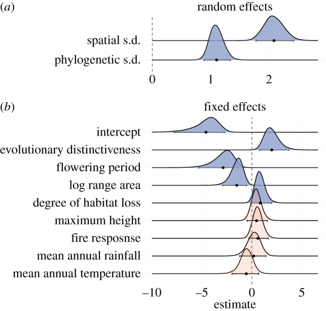
Bayesian marginal posterior distributions of model parameters. (a) shows the estimated standard deviation (s.d.) of the spatial and phylogenetic random effects calculated at the species level (see text). (b) shows the linear regression coefficients of fixed effects. Because all fixed-effect variables were standardized, these represent standardized coefficients and are comparable to one another. Posterior distributions that were categorized as substantial effects, (95% credible intervals do not overlap zero) are plotted as blue (top five); otherwise red (bottom four). The mean of the posteriors are plotted as points along with error bars representing the 95% credible interval. (Online version in colour.)

Three of the fixed factors in the model (ED, flowering period and log range area) had 95% credible intervals that did not overlap with zero (figure 3), and a fourth had a 95% confidence interval that only very slightly overlapped zero (habitat loss), suggesting a significant influence on threat probability independent of spatial and phylogenetic effects. The other factors we tested (height, fire response, temperature and rainfall) had posterior distributions with considerable overlap with zero. We therefore consider ED, flowering period, log range area and habitat loss to be potentially important determinants of threat probability.

Results for a standard phylogenetically informed model without spatial effects are given in the electronic supplementary material. The non-spatial model tended to underpredict extinction risk compared to our full spatiophylogenetic model (electronic supplementary material, figure S4), and it was unable to detect the contribution of habitat loss or range size to extinction risk, although it identified ED and flowering period length as predictors with similar effect sizes to the spatiophylogenetic model (electronic supplementary material, figure S5). The spatial model is also considerably better according to the Watanabe–Akaike information criterion (WAIC), with a WAIC of 78.44, as opposed to 131.63 for the non-spatial model.

In general, the model clearly distinguishes Hakea species currently classified as threatened from those classified as not threatened, with currently threatened species tending to have a predicted threat probability of greater than 0.2 (18 out of 19 threatened species), and those not currently threatened having predicted threat probability of less than 0.2 (figure 2). There are, however, two currently threatened species (Hakea macraena and Hakea dactyloides) for which the model returns a low threat probability (one just below the threshold and one just slightly above). Conversely, there are 11 species of Hakea that are currently not classified as threatened for which the model returns a threat probability of greater than 0.2 (figure 2): these are the species with high latent extinction risk that we classified as being ‘of concern’. Electronic supplementary material, figure S6b shows the geographical distribution of occurrence records for species of concern, alongside those for species currently threatened (electronic supplementary material, figure S6a). Currently threatened species are clustered into two regions of Australia heavily modified for agriculture: southeastern Australia and the wheatbelt region of southwestern Australia. Of concern species are also clustered in these two regions, but their distribution in southeastern Australia appears to be largely around the periphery of the region occupied by currently threatened species. In southwestern Australia, of concern species are distributed across the southwest Australian Floristic region, including both the inland wheatbelt zone and the coastal sandplain heathlands.

There is substantial variation among species in the relative contributions of the two random and four fixed risk factors to the predicted threat probability, although the influence of the fixed-effect factors tended to be larger than that of the random spatial and phylogenetic factors (electronic supplementary material, figure S7). Mapping the geographical patterns in the independent effect of each risk factor reveals a broad division between eastern and western Australia (see the electronic supplementary material, figure S8 for detailed maps).

4. Discussion

Our results support a growing body of evidence that threat status of plant species is determined by a combination of external threatening processes, species biology and factors captured by the evolutionary distinctiveness of species on their phylogeny. Our novel spatiophylogenetic method allows us to go beyond previous comparative analyses of extinction risk to distinguish the biological, geographical, phylogenetic and spatial contributions to threat status, for individual species as well as different geographical regions.

(a). Evolutionary distinctiveness and extinction risk

We found evidence for a link between greater ED of Hakea species and a higher probability of being threatened, the first evidence for such a link that is independent of both phylogenetic and spatial effects on patterns of threat status.

Although there is a growing list of taxa in which an association has been found between greater ED or evolutionary age and higher threat status [18–22,29,47], the explanations for this link remain speculative. Explanations are of two basic kinds [48]: (i) species ageing effects: with increasing time since divergence from sister species, predictable changes in a species geography or biology may increase susceptibility to extinction; and (ii) diversification effects: species on long terminal branches appear ‘old’ because they belong to clades that share their high extinction vulnerability, leading to high extinction rates that leave them relatively isolated on the tree of life (‘hidden extinction’ effect).

Some models of geographical range evolution suggest that species achieve their maximum range sizes at early or mid-stages of their lifespans, followed by an extended period of range contraction [23,49]. Hence, the association between species age and threat status could result from smaller ranges in older species. This explanation is unlikely in Hakea, because there was still a positive association between threat status and ED even after accounting for range area in the model. Additionally, ED was positively correlated with range size in our study (r = 0.2; electronic supplementary material, figure S10), suggesting older Hakea species tend to have larger ranges. This is consistent with evidence that range sizes tend to be larger in older species of the plant genus Psychotria [50]. Alternatively, other predictable biological changes, such as increasing ecological specialization with age [19], may account for the positive ED-threat association. In Hakea, species with narrower climatic niches tend to occupy smaller distributions, although the direction of causation is unclear [51], and again, any effect of ecological specialization on elevated extinction risk is unlikely to result simply from smaller range sizes. Whatever the mechanism that links ED with risk of extinction, this association is potentially important for conservation. Phylogenetically isolated species are valued for their distinctiveness, and ED is formally recognized as a criterion for conservation ranking under the evolutionarily distinct and globally endangered (EDGE) scheme [38], which additively combines ED with IUCN threat status. But if higher ED species also tend to be at greater risk of extinction, then the EDGE scheme may capture species with elevated sensitivity to human impacts, even if their true threat status is poorly known.

(b). Species biology and extinction risk

The strongest biological predictor of threat status in Hakea is length of flowering period––species with shorter periods in flower each year are more likely to be threatened. The same pattern has also been found in Banksia [15] and some other plant groups [2,48,52]. Longer flowering periods could be associated with greater seed set and recruitment, and hence larger populations, which might buffer plant species against disturbances [2]. Longer flowering periods may also contribute to flexibility in responding to anthropogenic stresses. This could be thought of as a temporal insurance effect, analogous to the spatial insurance effect thought to underlie the negative association between range size and extinction threat [53,54]. For example, plants with a short flowering period may be highly dependent on particular pollinators that become active around the same time. If these pollinators are at risk themselves, it limits the options available for reproduction. In fact, any threat processes that are temporally heterogeneous could increase the risk of interrupting reproduction for species with short flowering periods.

(c). Spatial patterns in the drivers of extinction risk

Our method allows us to estimate and account for the effects of spatial covariance when estimating other factors in the model. This is particularly important when extinction risk and drivers of extinction risk are likely to have spatial structure. A standard phylogenetically informed model without spatial effects was unable to detect the contribution of habitat loss or range size to extinction risk. This is likely because the spatial effect in our model picked up a broad east-to-west pattern of extinction risk that was independent of our measured environmental and threat factors. This effect normally obscures the effects of habitat loss and range size because both of these factors also show a broad east-west pattern of variation, with more extensive habitat loss and smaller ranges in the southwest biodiversity hotspot. Spatial patterns that remain unexplained by variables in the model (e.g. spatial error) may be more complex than those we found in this study, and our approach has the flexibility to tease those out (see the electronic supplementary material: simulations for details).

Our method uses the full extent of each species' range in analysing spatial patterns, rather than a single midpoint. A previous approach to addressing this problem used spatial eigenvectors and found that using the full range information led to superior performance and the detection of patterns that midpoint-based methods were unable to detect [55]. However, this previous approach has no explicit spatial model, and therefore, the spatial variation being modelled cannot be visualized, and predictions to novel areas would be challenging to make, whereas these are straightforward using our method. Additionally, spatial covariance in this previous model is based on co-occurrence of species, meaning that species with no range overlap will all be treated as having the same maximum distance from one another, regardless of whether their ranges are close or far apart. This makes it inappropriate for modelling unknown spatial risk factors across a landscape.

Our method also allows us to map the geographical patterns in the independent effects of different predictors of threat status. When spatial error is removed, the distribution of species assemblages with high threat probability predicted from the model shows a clear geographical pattern (electronic supplementary material, figure S8a). The two regions of highest predicted threat are centred on the central east coast and the southwest coast of Australia. This geographical pattern seems to be driven primarily by the pattern of threat predicted from flowering period alone (electronic supplementary material, figure S3c), with smaller contributions from the independent predictions of threat owing to habitat loss (electronic supplementary material, figure S3d), phylogenetic position (electronic supplementary material, figure S3e) and range size (electronic supplementary material, figure S3f). In fact, these two predicted ‘threat hotspots’ also overlap substantially with Australia's two global biodiversity hotspots (southwest Australia and forests of eastern Australia). Global biodiversity hotspots are defined on the basis of unusually high concentrations of endemic plant diversity, combined with high levels of anthropogenic land-use change [56]. Our results suggest that for Hakea, hotspots are additionally regions in which species have a tendency to be ‘inherently’ vulnerable, on the basis of a brief annual flowering period, small range size and their phylogenetic position. This coincidence of regions where (i) there is high endemic diversity, (ii) a high proportion of original habitat is already gone, and (iii) species are inherently vulnerable because of their biology, means that the two Australian hotspots are regions that should be afforded high priority for the protection of remaining natural habitat.

The independent effect of ED on threat status shows a largely complementary geographical pattern to those for flowering period and phylogeny (electronic supplementary material, figure S3). Here, it is the arid zone (including the inland and the south-central and west coasts) and the north of Australia which are the regions of highest predicted threat probability. This can probably be explained by the low species richness of these regions and the fact that a number of species (especially in the arid zone) are on the ends of long branches, which elevates ED in these regions. One apparent consequence of the almost complementary geographical patterns for ED and the other variables is that distributions of many of the species with high ‘latent risk’––species not yet threatened, but predicted by the model to be threatened––lie in the zones of overlap between regions of high threat predicted from ED and from the other variables (electronic supplementary material, figure S2). These are species we have classified as being ‘of concern’, because their inherent vulnerability could push them rapidly towards extinction if habitat loss or other ecosystem disturbances within their distributions increase.

The speed of environmental change means it is inevitable that many species currently considered stable or secure will become threatened in the future. If prevention is better than cure in conservation, as it is in medicine, then the ability to anticipate future species declines, so that preventative action can be taken, will be important. As an analytical tool for early identification of species inherently sensitive to human impacts, our INLA-based model could help to bring about a more proactive approach to conservation planning, extending the focus from currently threatened to potentially threatened biodiversity.

Data accessibility

All data necessary to reproduce the results of the study are available from the Dryad Digital Repository: https://dx.doi.org/10.5061/dryad.jh9w0vt73 [57].

A version of this manuscript has been previously posted as a preprint [58].

Authors' contributions

R.D. and M.C. conceived of the project. R.D. designed and carried out the statistical analysis. A.S. collected data. M.C. and R.D. wrote the manuscript and all authors contributed to editing the manuscript.

Competing interests

We declare we have no competing interests.

Funding

This research is supported by Australian Research Council Discovery grant no. DP160103942. A.S. is supported by the Australian Government Research Training Program.

References

- 1.International Union for Conservation of Nature. 2018. The IUCN Red List of threatened species, version 2018-1. See https://www.iucnredlist.org. Downloaded 20 March 2018.
- 2.Fréville H, McConway K, Dodd M, Silvertown J. 2007. Prediction of extinction in plants: interaction of extrinsic threats and life history traits. Ecology 88, 2662–2672. ( 10.1890/06-1453.1) [DOI] [PubMed] [Google Scholar]
- 3.Cardillo M, Mace GM, Gittleman JL, Jones KE, Bielby J, Purvis A. 2008. The predictability of extinction: biological and external correlates of decline in mammals. Proc. R. Soc. B 275, 1441–1448. ( 10.1098/rspb.2008.0179) [DOI] [PMC free article] [PubMed] [Google Scholar]
- 4.Fisher DO, Blomberg SP, Owens IPF. 2003. Extrinsic versus intrinsic factors in the decline and extinction of Australian marsupials. Proc. R. Soc. Lond. B 270, 1801–1808. ( 10.1098/rspb.2003.2447) [DOI] [PMC free article] [PubMed] [Google Scholar]
- 5.Cardillo M, Mace GM, Gittleman JL, Purvis A. 2006. Latent extinction risk and the future battlegrounds of mammal conservation. Proc. Natl Acad. Sci. USA 103, 4157–4161. ( 10.1073/pnas.0510541103) [DOI] [PMC free article] [PubMed] [Google Scholar]
- 6.Fisher DO, Owens IPF. 2004. The comparative method in conservation biology. Trends Ecol. Evol. (Amst.) 19, 391–398. ( 10.1016/j.tree.2004.05.004) [DOI] [PubMed] [Google Scholar]
- 7.Purvis A, Cardillo M, Grenyer R, Collen B. 2005. Correlates of extinction risk: phylogeny, biology, threat and scale. In Phylogeny and conservation (eds Purvis A, Gittleman JL, Brooks T), pp. 295–316. Cambridge, UK: Cambridge University Press. [Google Scholar]
- 8.Purvis A. 2008. Phylogenetic approaches to the study of extinction. Annu. Rev. Ecol. Evol. Syst. 39, 301–319. ( 10.1146/annurev-ecolsys-063008-102010) [DOI] [Google Scholar]
- 9.Murray BR, Thrall PH, Gill AM, Nicotra AB. 2002. How plant life-history and ecological traits relate to species rarity and commonness at varying spatial scales. Austral. Ecol. 27, 291–310. ( 10.1046/j.1442-9993.2002.01181.x) [DOI] [Google Scholar]
- 10.Murray KA, Verde Arregoitia LD, Davidson A, Di Marco M, Di Fonzo MMI. 2014. Threat to the point: improving the value of comparative extinction risk analysis for conservation action. Glob. Change Biol. 20, 483–494. ( 10.1111/gcb.12366) [DOI] [PubMed] [Google Scholar]
- 11.Godefroid S. 2014. Do plant reproductive traits influence species susceptibility to decline? Plant Ecol. Evol. 147, 154–164. ( 10.5091/plecevo.2014.863) [DOI] [Google Scholar]
- 12.Sjostrom A, Gross CL. 2006. Life-history characters and phylogeny are correlated with extinction risk in the Australian angiosperms. J. Biogeogr. 33, 271–290. ( 10.1111/j.1365-2699.2005.01393.x) [DOI] [Google Scholar]
- 13.Sodhi NS, et al. 2008. Correlates of extinction proneness in tropical angiosperms. Divers. Distrib. 14, 1–10. ( 10.1111/j.1472-4642.2007.00398.x) [DOI] [Google Scholar]
- 14.Leão TCC, Fonseca CR, Peres CA, Tabarelli M. 2014. Predicting extinction risk of Brazilian Atlantic forest angiosperms. Conserv. Biol. 28, 1349–1359. ( 10.1111/cobi.12286) [DOI] [PubMed] [Google Scholar]
- 15.Cardillo M, Skeels A. 2016. Spatial, phylogenetic, environmental and biological components of variation in extinction risk: a case study using Banksia. PLoS ONE 11, e0154431 ( 10.1371/journal.pone.0154431) [DOI] [PMC free article] [PubMed] [Google Scholar]
- 16.Davies TJ. 2019. The macroecology and macroevolution of plant species at risk. New Phytol. 222, 708–713. ( 10.1111/nph.15612) [DOI] [PubMed] [Google Scholar]
- 17.Redding DW, Mazel F, Mooers AØ. 2014. Measuring evolutionary isolation for conservation. PLoS ONE 9, e113490 ( 10.1371/journal.pone.0113490) [DOI] [PMC free article] [PubMed] [Google Scholar]
- 18.Johnson CN, Delean S, Balmford A. 2002. Phylogeny and the selectivity of extinction in Australian marsupials. Anim. Conserv. 5, 135–142. ( 10.1017/S1367943002002196) [DOI] [Google Scholar]
- 19.Meijaard E, Sheil D, Marshall AJ, Nasi R. 2007. Phylogenetic age is positively correlated with sensitivity to timber harvest in Bornean mammals. Biotropica 40, 76–85. ( 10.1111/j.1744-7429.2007.00340.x) [DOI] [Google Scholar]
- 20.Vamosi JC, Wilson JR. U. 2008. Nonrandom extinction leads to elevated loss of angiosperm evolutionary history. Ecol. Lett. 11, 1047–1053. ( 10.1111/j.1461-0248.2008.01215.x) [DOI] [PubMed] [Google Scholar]
- 21.Redding DW, DeWolff CV, Mooers AØ. 2010. Evolutionary distinctiveness, threat status, and ecological oddity in primates. Conserv. Biol. 24, 1052–1058. ( 10.1111/j.1523-1739.2010.01532.x) [DOI] [PubMed] [Google Scholar]
- 22.Verde Arregoitia LD, Blomberg SP, Fisher DO. 2013. Phylogenetic correlates of extinction risk in mammals: species in older lineages are not at greater risk. Proc. R. Soc. B 280, 20131092 ( 10.1098/rspb.2013.1092) [DOI] [PMC free article] [PubMed] [Google Scholar]
- 23.Willis JC. 1922. Age and area: a study in geographical distribution and origin of species by J. C. Willis, with chapters by Hugo de Vries, HB Guppy, Mrs E. M. Reid, James Small. Cambridge, UK: Cambridge University Press. [Google Scholar]
- 24.Wilson EO. 1961. The nature of the taxon cycle in the Melanesian ant fauna. Am. Nat. 95, 169–193. ( 10.1086/282174) [DOI] [Google Scholar]
- 25.Ricklefs RE, Bermingham E. 2002. The concept of the taxon cycle in biogeography. Global Ecol. Biogeogr. 11, 353–361. ( 10.1046/j.1466-822x.2002.00300.x) [DOI] [Google Scholar]
- 26.Bromham L, Hua X, Cardillo M. 2016. Detecting macroevolutionary self-destruction from phylogenies. Syst. Biol. 65, 109–127. ( 10.1093/sysbio/syv062) [DOI] [PubMed] [Google Scholar]
- 27.Tanentzap AJ, Igea J, Johnston MG, Larcombe MJ. 2018. Range size dynamics can explain why evolutionarily age and diversification rate correlate with contemporary extinction risk in plants. bioRxiv 152215 ( 10.1101/152215) [DOI]
- 28.Davies TJ, et al. 2011. Extinction risk and diversification are linked in a plant biodiversity hotspot. PLoS Biol. 9, e1000620 ( 10.1371/journal.pbio.1000620) [DOI] [PMC free article] [PubMed] [Google Scholar]
- 29.Gaston KJ, Blackburn TM. 1997. Evolutionary age and risk of extinction in the global avifauna. Evol. Ecol. 11, 557–565. ( 10.1007/s10682-997-1511-4) [DOI] [Google Scholar]
- 30.Safi K, Pettorelli N. 2010. Phylogenetic, spatial and environmental components of extinction risk in carnivores. Global Ecol. Biogeogr. 19, 352–362. ( 10.1111/j.1466-8238.2010.00523.x) [DOI] [Google Scholar]
- 31.Jetz W, Freckleton RP. 2015. Towards a general framework for predicting threat status of data-deficient species from phylogenetic, spatial and environmental information. Phil. Trans. R. Soc. B 370, 20140016 ( 10.1098/rstb.2014.0016) [DOI] [PMC free article] [PubMed] [Google Scholar]
- 32.Freckleton RP, Jetz W. 2009. Space versus phylogeny: disentangling phylogenetic and spatial signals in comparative data. Proc. R. Soc. B 276, 21–30. ( 10.1098/rspb.2008.0905) [DOI] [PMC free article] [PubMed] [Google Scholar]
- 33.Skeels A, Cardillo M. 2017. Environmental niche conservatism explains the accumulation of species richness in Mediterranean-hotspot plant genera. Evolution 71, 582–594. ( 10.1111/evo.13179) [DOI] [PubMed] [Google Scholar]
- 34.Fick SE, Hijmans RJ. 2017. WorldClim 2: new 1-km spatial resolution climate surfaces for global land areas. Int. J. Climatol. 37, 4302–4315. ( 10.1002/joc.5086) [DOI] [Google Scholar]
- 35.Price SA, Gittleman JL. 2007. Hunting to extinction: biology and regional economy influence extinction risk and the impact of hunting in artiodactyls. Proc. R. Soc. B 274, 1845–1851. ( 10.1098/rspb.2007.0505) [DOI] [PMC free article] [PubMed] [Google Scholar]
- 36.Davidson AD, Hamilton MJ, Boyer AG, Brown JH, Ceballos G. 2009. Multiple ecological pathways to extinction in mammals. Proc. Natl Acad. Sci. USA 106, 10 702–10 705. ( 10.1073/pnas.0901956106) [DOI] [PMC free article] [PubMed] [Google Scholar]
- 37.Cardillo M, Weston PH, Reynolds ZKM, Olde PM, Mast AR, Lemmon EM, Lemmon AR, Bromham L. 2017. The phylogeny and biogeography of Hakea (Proteaceae) reveals the role of biome shifts in a continental plant radiation. Evolution 71, 1928–1943. ( 10.1111/evo.13276) [DOI] [PubMed] [Google Scholar]
- 38.Isaac NJ. B., Turvey ST, Collen B, Waterman C, Baillie JE. M. 2007. Mammals on the EDGE: conservation priorities based on threat and phylogeny. PLoS ONE 2, e296 ( 10.1371/journal.pone.0000296) [DOI] [PMC free article] [PubMed] [Google Scholar]
- 39.Kembel SW, Cowan PD, Helmus MR, Cornwell WK, Morlon H, Ackerly DD, Blomberg SP, Webb CO. 2010. Picante: R tools for integrating phylogenies and ecology. Bioinformatics 26, 1463–1464. ( 10.1093/bioinformatics/btq166) [DOI] [PubMed] [Google Scholar]
- 40.Barker RM, Haegi L, Barker WR. 1999. Hakea. In Flora of Australia, vol. 178 (ed. Wilson A.), pp. 31–169. Canberra, Australia: ABRS/CSIRO. [Google Scholar]
- 41.Dinnage R, Cardillo M. 2018. Habitat loss is information loss: species distribution models are compromised in anthropogenic landscapes. bioRxiv 258038. ( 10.1101/258038) [DOI]
- 42.Rue H, Martino S, Chopin N. 2009. Approximate Bayesian inference for latent Gaussian models by using integrated nested Laplace approximations. J. R. Stat. Soc. B 71, 319–392. ( 10.1111/j.1467-9868.2008.00700.x) [DOI] [Google Scholar]
- 43.Martins TG, Simpson D, Lindgren F, Rue H. 2013. Bayesian computing with INLA: new features. Comput. Stat. Data Anal. 67, 68–83. ( 10.1016/j.csda.2013.04.014) [DOI] [Google Scholar]
- 44.Illian JB, Sørbye SH, Rue H. 2012. A toolbox for fitting complex spatial point process models using integrated nested Laplace approximation (INLA). Ann. Appl. Stat. 6, 1499–1530. ( 10.1214/11-AOAS530) [DOI] [Google Scholar]
- 45.Grafen A. 1989. The phylogenetic regression. Phil. Trans. R. Soc. Lond. B 326, 119–157. ( 10.1098/rstb.1989.0106) [DOI] [PubMed] [Google Scholar]
- 46.Li D, Nell L, Ives AR, Dinnage R, Mikryukov V. 2019. daijiang/phyr: CRAN v1.0.2. Zenodo ( 10.5281/zenodo.3550309) [DOI]
- 47.Greenberg DA, Palen WJ, Chan KC, Jetz W, Mooers AØ. 2018. Evolutionarily distinct amphibians are disproportionately lost from human-modified ecosystems. Ecol. Lett. 21, 1530–1540. ( 10.1111/ele.13133) [DOI] [PubMed] [Google Scholar]
- 48.Lahti T, Kemppainen E, Kurtto A, Uotila P. 1991. Distribution and biological characteristics of threatened vascular plants in Finland. Biol. Conserv. 55, 299–314. ( 10.1016/0006-3207(91)90034-7) [DOI] [Google Scholar]
- 49.de Moraes Weber M, Stevens RD, Lorini ML, Grelle CE. V. 2014. Have old species reached most environmentally suitable areas? A case study with South American phyllostomid bats. Glob. Ecol. Biogeogr. 23, 1177–1185. ( 10.1111/geb.12198) [DOI] [Google Scholar]
- 50.Paul JR, Morton C, Taylor CM, Tonsor SJ. 2009. Evolutionary time for dispersal limits the extent but not the occupancy of species' potential ranges in the tropical plant genus Psychotria (Rubiaceae). Am. Nat. 173, 188–199. ( 10.1086/595762) [DOI] [PubMed] [Google Scholar]
- 51.Cardillo M, Dinnage R, McAlister W. 2019. The relationship between environmental niche breadth and geographic range size across plant species. J. Biogeogr. 46, 97–109. ( 10.1111/jbi.13477) [DOI] [Google Scholar]
- 52.Ames GM, Wall WA, Hohmann MG, Wright JP. 2017. Trait space of rare plants in a fire-dependent ecosystem. Conserv. Biol. 31, 903–911. ( 10.1111/cobi.12867) [DOI] [PubMed] [Google Scholar]
- 53.Keith DA, et al. 2013. Scientific foundations for an IUCN Red List of ecosystems. PLoS ONE 8, e62111 ( 10.1371/journal.pone.0062111) [DOI] [PMC free article] [PubMed] [Google Scholar]
- 54.Loreau M, Mouquet N, Gonzalez A. 2003. Biodiversity as spatial insurance in heterogeneous landscapes. Proc. Natl Acad. Sci. USA 100, 12 765–12 770. ( 10.1073/pnas.2235465100) [DOI] [PMC free article] [PubMed] [Google Scholar]
- 55.Morales-Castilla I, Rodríguez MÁ, Kaur R, Hawkins BA. 2013. Range size patterns of New World oscine passerines (Aves): insights from differences among migratory and sedentary clades. J. Biogeogr. 40, 2261–2273. ( 10.1111/jbi.12159) [DOI] [Google Scholar]
- 56.Myers N, Mittermeier RA, Mittermeier CG, da Fonseca GA, Kent J. 2000. Biodiversity hotspots for conservation priorities. Nature 403, 853–858. ( 10.1038/35002501) [DOI] [PubMed] [Google Scholar]
- 57.Dinnage R, Skeels A, Cardillo M. 2020. Data from: Spatiophylogenetic modelling of extinction risk reveals evolutionary distinctiveness and brief flowering period as threats in a hotspot plant genus Dryad Digital Repository. ( 10.5061/dryad.jh9w0vt73) [DOI] [PMC free article] [PubMed]
- 58.Dinnage R, Skeels A, Cardillo M. 2018. Spatiophylogenetic modelling of extinction risk reveals evolutionary distinctiveness and brief flowering period as risk factors in a diverse hotspot plant genus BioRxiv 496547 ( 10.1101/496547) [DOI] [PMC free article] [PubMed]
Associated Data
This section collects any data citations, data availability statements, or supplementary materials included in this article.
Data Citations
- Dinnage R, Skeels A, Cardillo M. 2020. Data from: Spatiophylogenetic modelling of extinction risk reveals evolutionary distinctiveness and brief flowering period as threats in a hotspot plant genus Dryad Digital Repository. ( 10.5061/dryad.jh9w0vt73) [DOI] [PMC free article] [PubMed]
- Dinnage R, Skeels A, Cardillo M. 2018. Spatiophylogenetic modelling of extinction risk reveals evolutionary distinctiveness and brief flowering period as risk factors in a diverse hotspot plant genus BioRxiv 496547 ( 10.1101/496547) [DOI] [PMC free article] [PubMed]
Supplementary Materials
Data Availability Statement