Abstract
Soil organic matter (SOM) refers to all carbon-containing organic matter in soil and is one of the most important indicators of soil fertility. The hyperspectral inversion analysis of SOM traditionally relies on laboratory chemical testing methods, which have the disadvantages of being inefficient and time-consuming. In this study, 69 soil samples were collected from the Honghu farmland area and a mining area in northwest China. After pretreatment, 10 spectral indicators were obtained. Ridge regression, kernel ridge regression, Bayesian ridge regression, and AdaBoost algorithms were then used to construct the SOM hyperspectral inversion model based on the characteristic bands, and the accuracy of the models was compared. The results showed that the AdaBoost algorithm based on a grid search had the best accuracy in the different regions. For the mining area in northwest China, = 0.91, = 0.22, and = 0.2. For the Honghu farmland area, = 0.86, = 0.72, and = 0.56. The detection of SOM content using hyperspectral technology has the characteristics of a high detection precision and high speed, which will be of great significance for the rapid development of precision agriculture.
Keywords: hyperspectral remote sensing, soil organic matter, AdaBoost algorithm, pearson correlation analysis
1. Introduction
Soil organic matter (SOM) is an important part of soil. It promotes plant growth and improves the physical properties of soil. It plays a very important role in promoting the formation of soil structure, improving the physical properties of soil and soil’s ability to retain fertilizer, and is the main limiting factor for crop yield [1,2]. Therefore, rapid and accurate monitoring of SOM is of great significance for soil fertility monitoring and agricultural development. The traditional methods for the determination of soil organic matter are still widely used because of their high precision. However, these methods are usually time-consuming, laborious, harmful, or polluting, and it is difficult to directly determine results in the field. Additionally, the traditional method is based on point measurement, which has few measuring points, a slow speed, a limited scope, and cannot meet the requirements of precision fertilization technology and precision agriculture regarding the spatial-temporal variation of soil organic matter [3]. The methods based on spectroscopy have the characteristics of high efficiency, wide coverage, low cost, and they can be used to effectively determine the SOM content. However, in the original spectrum acquisition process, due to factors such as the collection environment and the instrument itself, a large amount of irrelevant redundant information will appear. This greatly affects the prediction accuracy and the robustness of the model. Therefore, data reduction and reduction of unrelated information for the original spectral information is an important prerequisite and the basis for constructing quantitative inversion models [4,5].
Since the 1960s, the quantitative inversion of the reflectance spectra of soil organic matter has been carried out around the world. Nawar et al. [6] studied the soil of the Sinai Peninsula in Egypt, using Savitzky–Golay (SG) smoothing, first-order derivative (FD), second-order derivative (SD), continuum removal (CR), and standard normal variate detrend (SNV-D) transformations. Multiplicative scatter correction (MSC) and extended MSC were used to preprocess the original spectra. Partial least squares regression (PLSR), support vector regression (SVM), and multiple adaptive regression splines (MARS) were used to determine the best method for assessing the SOM and clay content in soil affected by salt. The results showed that the MARS model outperformed the PLSR and SVM models, and the MARS model after a CR treatment obtained the best prediction results. Steinberg et al. [7] analyzed the absorption characteristics of the spectral curves of soils with different organic matter contents and concluded that the PLSR model established by the logarithmic processing of the removal of the envelope line and the reciprocal of the reflectance had the best prediction effect.
However, in visible and near-infrared spectroscopy (Vis/NIRS, 350–2500 nm), the reflectance of the soil spectrum is generally low. The absorption characteristics are not significant and they are easily affected by the external environment; therefore, the extension of the inversion model established by directly using the measured spectrum is limited. The spectral reflectance of soil is a comprehensive response to the spectral behavior of soil’s inherent physical and chemical properties. Different types of soil have different spectral characteristics due to different physical and chemical properties. Additionally, even for the same type of soil, different parent materials affect their spectral characteristics. Therefore, by studying different types of soil, the prediction model of organic matter content obtained by using the combined spectral index model is of great significance for studying the generalization ability of the model.
Therefore, in this study, we selected the characteristic bands based on different spectral index transformations and the Pearson correlation analysis method, where the bands with a correlation coefficient of greater than 0.7 were selected as the characteristic bands. Then, ridge regression (RR), kernel ridge regression (KRR), bayesian ridge regression (BRR), and adaBoost algorithms were used to establish the inversion model. The quantitative inversion method for SOM lays a foundation for the use of hyperspectral remote sensing imagery for soil fertility monitoring and agricultural development.
2. Materials and Methods
2.1. Study Areas
Two sites were selected for soil sampling, where one was a mining area and the other was farmland. The mining area soil was collected from northwest China. The area belongs to the northern temperate continental climate. It has rich mineral resources, four distinct seasons, and abundant sunshine. The area has the natural advantages of water, soil, light, and heat resources for the development of agriculture. The main soil types in this area are alluvial soils and irrigated soils, which are formed under the influence of long-term cultivation, fertilization, and irrigation.
The farmland soil was collected from Yanwo Town of the city of Honghu, China, which is under the jurisdiction of the city of Jingzhou, Hubei province. The economy in this area is mainly based on agriculture, particularly rice, sesame, cotton, wheat, and other crops. The area features a subtropical humid monsoon climate, abundant sunshine, abundant rainfall, and excellent water resources, but floods are prone to occur in summer. Agricultural cultivation in this area has a long history.
2.2. Research Methods
2.2.1. Ridge Regression
The ridge regression (RR) method is a biased estimation method for the analysis of multicollinear data [8,9]. At the cost of the partial precision of the least-squares regression equation, a regression equation with a strong tolerance to ill-conditioned data is obtained, which can better solve the problem of the collinearity of hyperspectral data.
| (1) |
Here, is the parameter of ridge estimate, is the P-order unit matrix, and is the number of modeling samples.
2.2.2. Kernel Ridge Regression
Kernel ridge regression (KRR) is a regression analysis model that combines ridge regression with kernel techniques [10]. For a nonlinear kernel, this corresponds to a nonlinear function in the original space. Kernel regression has an approximate solution and is highly efficient when used on moderate-scale data.
| (2) |
Here, is the regularization term. Once again, to generalize this model to non-linear cases, a kernel trick is applied, which maps the data into a higher-dimensional space.
2.2.3. Bayesian Ridge Regression
Bayesian ridge regression (BRR) is a machine learning regression algorithm based on Bayesian theory [11,12]. Bayesian linear regression is shown in Equation (3). Its purpose is to find the parameter vector distribution that makes the loss function (Equation (4)) the smallest.
| (3) |
| (4) |
Here, n is the dimension of sample space, m is the sample capacity, is the parameter vector, is the nonlinear function of input vector x, and the prior probability of is given in Equation (5):
| (5) |
According to Bayesian rules:
| (6) |
where:
| (7) |
such that:
| (8) |
where is a posterior probability, is a constant independent of , c is a constant, and the prior probability corresponds to the L2 regular term in the ridge regression, and is thus called Bayesian ridge regression.
2.2.4. AdaBoost Algorithm
The basic process of the AdaBoost algorithm is to train a group of component regressions in turn, in which the training set of each component regression is composed of the most informative samples given by the other component regressions. Finally, these component regressions are integrated with a linear weighting to obtain the final decision result [13]. The method for selecting the “richest information” sample is as follows. Each training sample is given a weight indicating the probability of it being selected for the training set by a component regression. For the regression prediction algorithms, first give a set of data sets , the initialization sample weight is , where n is the number of samples of the data set, and the weight set of the weak model is , where m is the number of weak models constructed. The model error rate is calculated, assuming that the prediction class sequence of the training data set of the weak model M1 is P1, and the loss function of the prediction type sequence of the linear prediction data set is Pre_1.
| (9) |
| (10) |
The error rate formula, which is the weight of the weak model P1, is expressed as:
| (11) |
The sample weights are updated using:
| (12) |
Through successive iterations, different prediction results pre_1, pre_2, ..., pre_m and the weight set P of the model are obtained. When the maximum iteration number is satisfied and the iteration is stopped, the regression prediction result is expressed as:
| (13) |
2.2.5. AdaBoost Algorithm Optimized Using a Grid Search
A grid search is a kind of original digital programming method used to solve constrained nonlinear extremum problems. It also has no special requirements for functions [14]. Its optimization method involves dividing the problem into network lines within a certain range. The advantage of the grid search method is that it can search for several parameter values at the same time, eventually obtaining the optimal parameter combination for the evaluation function. In the process of optimization, the parameters of each group are decoupled from each other, which can avoid the problem of multiple solutions caused by many parameters or coupling between parameters, it is convenient for parallel calculation, and has a high efficiency.
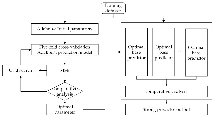
The prediction results of the AdaBoost algorithm are closely related to the base regression, the learning rate, the loss function, and the number of base regression loops; therefore, obtaining the optimal parameters is a critical step [15]. The grid search method first collects all possible parameter values and then groups them. Using the cross-validation grid search method, within the scope of the set of optimal model parameters, the mean square error (MSE) is compared for each forecast model such that it establishes the best prediction model that avoids the problem of the low accuracy of the original model. The flow of the AdaBoost algorithm based on grid search optimization is shown in Figure 1.
Figure 1.
AdaBoost algorithm flowchart based on a grid search. MSE: Mean square error.
2.2.6. Accuracy Evaluation
In this study, the three parameters selected to measure the accuracy of the evaluation models were the determination coefficient (R2), the root mean square error (RMSE), and the mean absolute error (MAE) [16]. The closer R2 is to 1, the higher the model fit and the more stable the model. The smaller the RMSE and MAE are, the higher the model prediction ability and the higher the model robustness. The larger R2 is, the smaller the RMSE and MAE are, and the higher the overall accuracy of the model [17].
| (14) |
| (15) |
| (16) |
Here, n is the number of samples, is the measured value, is the predicted value, and is the average of the measured values.
3. Results and Discussion
3.1. Soil Collection Preparation and Physical and Chemical Analysis
GPS positioning was adopted for the field collection of soil samples, where the coordinates of the actual sampling points and the detailed characteristic information of the sample plots were recorded. The surface soil with a depth of 0–20 cm was taken for each sample plot. To reduce the impact of rainfall and other factors, there was no precipitation in the first week of field sampling in the region and all sampling was completed within 1 days. According to the research needs, 41 samples were collected in the Honghu area and 28 samples were collected in northwest China [18]. After airdrying and sieving, the content of soil organic matter was determined using a potassium bichromate titrimetric method.
3.2. Spectral Reflectance Measurement
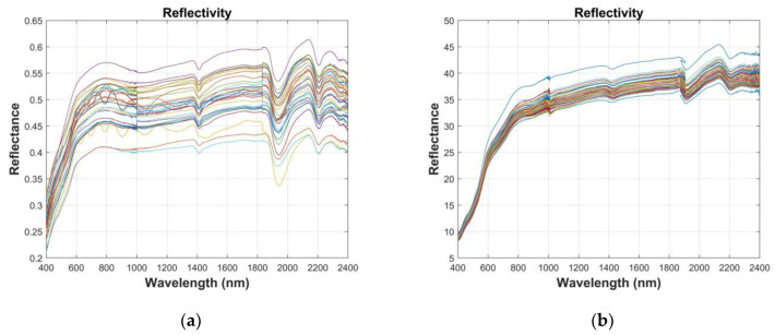
The indoor spectral measurement was undertaken with an ASD FieldSpec 3 spectrometer (Analytical Spectral Devices Inc., Boulder, CO, USA). Its wavelength range is 350–2500 nm and its spectral resolution is 1 nm. The soil samples were placed in dark Petri dishes and the surface of the soil samples was scraped with a ruler. The light source was a halogen lamp with a power of 1000 W. The probe was positioned perpendicular to the soil surface, 10 cm above the surface layer [19]. Each soil sample was calibrated using a standard reference whiteboard before the spectral measurement to obtain a baseline [20]. To ensure the accuracy of the data, the reflectivity was measured in four directions (three rotations in the same direction, 90° each time), and each spectral curve was measured and averaged 10 times. The arithmetic mean of the four spectra was taken as the actual reflection spectrum data of the soil sample and the average reflectance of each soil sample was taken as the original reflectance spectrum value, which was done to reduce the interference and external noise. As can be seen in Figure 2, for each soil sample, we removed the noisy edge bands from 350–399 nm and 2400–2500 nm, and we retained the 400–2399 nm bands for the modeling analysis [21].
Figure 2.
Soil reflectance spectra (with fringe noise removed): (a) northwest China and (b) Honghu.
3.3. Calibration Set and Validation Set
Before the modeling, the samples needed to be grouped. The 69 soil samples from the two research areas of northwest China and Honghu were divided according to a 3:1 ratio for the calibration set and validation set. The division of the calibration set and validation set was done using sample set partitioning based on the joint x-y distance (SPXY) method [22]. As can be seen from Table 1, 19 modeling sets and 9 validation sets were selected for the northwest China region, and 29 modeling sets and 12 validation sets were selected for the Honghu region.
Table 1.
Statistical characteristics of soil organic matter.
| Study Area | Sample Type | Number | Minimum | Maximum | Mean | SD | CV (%) | Skewness | Kurtosis |
|---|---|---|---|---|---|---|---|---|---|
| Northwest China | Entire | 28 | 3.43 | 7.34 | 4.6 | 0.8 | 17.4 | 1.47 | 4.1 |
| Honghu | Entire | 41 | 13.22 | 21.83 | 18.36 | 1.83 | 9.97 | −0.46 | 0.4 |
3.4. Spectral Pretreatment
The spectral data were unstable due to the instrument itself and the data were inevitably affected by factors such as the test environment, the sample background, the observation angle, the smoothness of the sample surface, and stray light during the spectral acquisition process [23]. There are many methods used for spectral transformation processing. However, there is no transformation method suitable for each component. Therefore, it is necessary to try a variety of mathematical transformation methods to find the best treatment for a particular study [24].
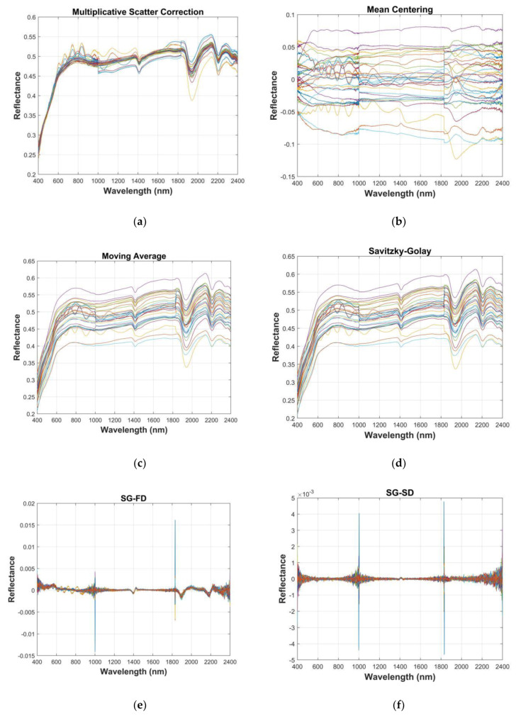
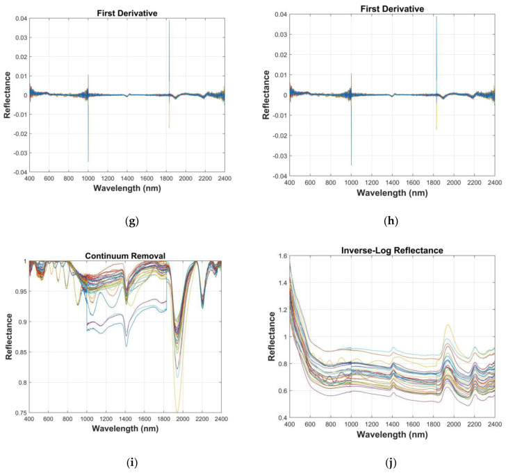
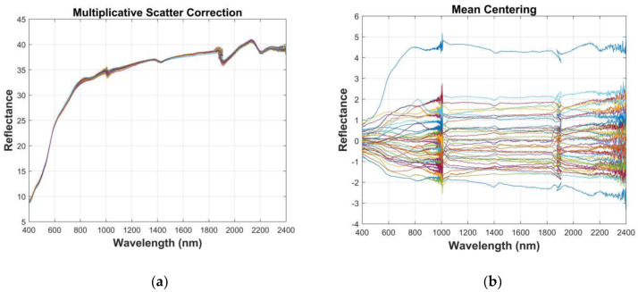
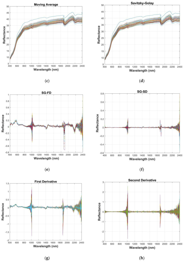
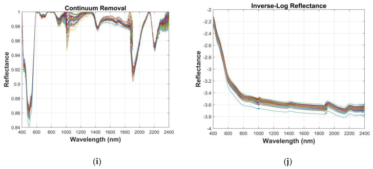
It can be seen from Figure 3 (northwest China) and Figure 4 (Honghu) that the influence of parallel noise could be eliminated through differential processing of the spectral curve [24]. Ten spectral indicators were obtained: inverse-log reflectance (Log(1/R)), continuum removal (CR), multiplicative scatter correction (MSC), first derivative reflectance (FDR), second derivative reflectance (SDR), Savitzky–Golay (SG), first derivative after Savitzky–Golay (SG-FD), second derivative after Savitzky–Golay (SG-SD), moving average (MA), and mean centering (MC). The overlapped samples were separated to extract the spectral information, where there was little difference from the original data. Using the CR method to effectively restrain the background spectrum amplified the absorption spectrum information [25,26]. Generally speaking, by using 10 kinds of spectral preprocessing methods, the information of the spectral data was expanded to varying degrees.
Figure 3.
Soil pretreatment under different spectral indices (northwest China): (a) multiplicative scatter correction (MSC), (b) mean centering (MC), (c) moving average (MA), (d) Savitzky–Golay (SG), (e) first derivative after Savitzky–Golay (SG-FD), (f) second derivative after Savitzky–Golay (SG-SD), (g) first derivative (FD), (h) second derivative (SD), (i) continuum removal (CR), and (j) inverse-log reflectance (Log(1/R)).
Figure 4.
Soil pretreatment under different spectral indices (Honghu): (a) multiplicative scatter correction (MSC), (b) mean centering (MC), (c) moving average (MA), (d) Savitzky–Golay (SG), (e) first derivative after Savitzky–Golay (SG-FD), (f) second derivative after Savitzky–Golay (SG-SD), (g) first derivative (FD), (h) second derivative (SD), (i) continuum removal (CR), and (j) inverse-log reflectance (Log(1/R)).
3.5. Characteristic Band Selection
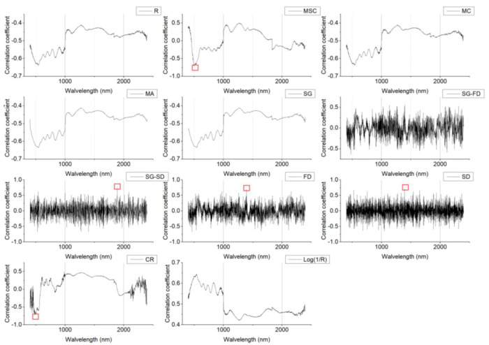
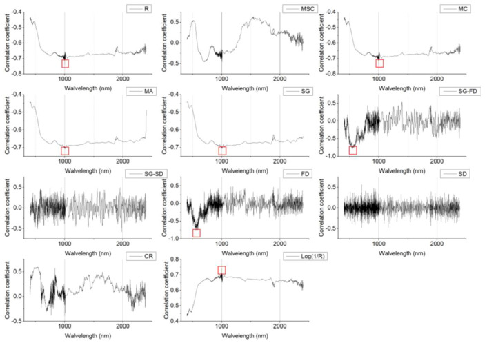
In this study, correlation analysis was carried out between the SOM content and the spectral transformation forms (MSC, MC, MA, SG, SG-FD, SG-SD, FD, SD, CR, Log(1/R)), as shown in Figure 5 and Figure 6. As can be seen in Figure 5, there was a certain degree of correlation between the SOM content and the smooth spectral reflectivity data, as well as the transformation form. The MSC spectra showed the largest negative correlations at 497 nm, 503 nm, and 504 nm, where the correlation coefficients were all greater than 0.7. Compared with the original spectrum, the SOM content was more closely correlated with the spectral data of the transformation forms. The correlation coefficient between the FD and SD spectra was the highest at 1393 nm and 1392 nm, where the correlation coefficients were 0.7 and 0.71. The SG-SD spectrum reached its highest positive correlation at 1888 nm, with a correlation coefficient of 0.76. The CR spectrum showed the largest negative correlation at 479 nm, 482 nm, and 487 nm, where the correlation coefficients were greater than 0.7. As can be seen in Figure 6, the spectral characteristic bands of the Honghu farmland showed different information. R, MC, MA, SG, and Log(1/R) showed good correlations in the range 974.1–1015.2 nm, the FD spectrum showed its highest negative correlation in the range 541.2–595.5 nm, and the SG-FD spectrum showed its highest negative correlation in the range 515.9–588 nm.
Figure 5.
Changes in the soil organic matter (SOM) content and correlation coefficients represented using different spectral indices (Northwest China).
Figure 6.
Changes in the SOM content and correlation coefficients represented using different spectral indices (Honghu area).
According to the results of the single-band correlation analysis, as can be seen from Table 2, bands with an absolute correlation value greater than 0.7 were selected as the characteristic bands, where the corresponding mathematical transformation of the soil spectrum was used as the independent variable and the SOM content was used as the dependent variable to establish the hyperspectral quantitative prediction model of the SOM content.
Table 2.
The feature bands and the correlation coefficients.
| Study Area | Spectral Index | Characteristic Band Number |
Characteristic Band Wavelengths (nm) | Maximum Correlation Coefficient |
Minimum Correlation Coefficient |
|---|---|---|---|---|---|
| Northwest China | R | 0 | 0.64 | 0.41 | |
| MSC | 3 | 497, 503, 504 | 0.70 | 0.00 | |
| MC | 0 | 0.64 | 0.41 | ||
| MA | 0 | 0.64 | 0.41 | ||
| SG | 0 | 0.64 | 0.41 | ||
| SG-FD | 0 | 0.64 | 0.00 | ||
| SG-SD | 1 | 1888 | 0.76 | 0.00 | |
| FD | 1 | 1393 | 0.70 | 0.00 | |
| SD | 1 | 1392 | 0.71 | 0.00 | |
| CR | 3 | 479, 482, 487 | 0.73 | 0.00 | |
| Log(1/R) | 0 | 0.64 | 0.42 | ||
| Honghu | R | 10 | 974.1–1009.2 | 0.74 | 0.43 |
| MSC | 0 | 0.64 | 0.00 | ||
| MC | 10 | 974.1–1009.2 | 0.74 | 0.43 | |
| MA | 13 | 994.8–1015.2 | 0.71 | 0.44 | |
| SG | 17 | 993.9–1011.2 | 0.71 | 0.44 | |
| SG-FD | 27 | 515.9–588 | 0.79 | 0.00 | |
| SG-SD | 0 | 0.58 | 0.00 | ||
| FD | 7 | 541.2–595.5 | 0.76 | 0.00 | |
| SD | 0 | 0.57 | 0.00 | ||
| CR | 0 | 0.60 | 0.00 | ||
| Log(1/R) | 9 | 974.1–1006.5 | 0.74 | 0.43 |
3.6. Regression Model
To select the optimal regression model, RR, KRR, BRR, and AdaBoost regression were used in the comparison. Each regression model was set with the default parameters. The SOM content was used as the dependent variable and the measured spectrum was used as the independent variable to construct the regression model. The results are shown in Table 3, which show that: (1) by comparing eight regression models in two regions, it can be seen from the accuracy of the validation set that for northwest China, BRR achieved the best accuracy, while for the Honghu area, RR achieved the best accuracy; and (2) the Adaboost algorithm for unjoined grid search optimization performed the worst in different regions.
Table 3.
Results of the quantitative inversion models of SOM.
| Study Area | Characteristic Bands | Models | |||
|---|---|---|---|---|---|
| Northwest China | MSC497, MSC503, MSC504, SG-SD1888, FD1393, SD1392, CR479, CR482, CR487 | RR | 0.78 | 0.25 | 0.22 |
| KRR | 0.87 | 0.20 | 0.16 | ||
| BRR | 0.90 | 0.18 | 0.14 | ||
| AdaBoost | 0.58 | 0.36 | 0.28 | ||
| Honghu | R974.1–1009.2, MC974.1–1009.2, MA994.8–1015.2, SG993.9–1011.2, SG-FD515.9–588, FD541.2–595.5, Log(1/R)974.1–1006.5 | RR | 0.85 | 0.74 | 0.54 |
| KRR | 0.77 | 0.93 | 0.68 | ||
| BRR | 0.84 | 0.78 | 0.63 | ||
| AdaBoost | 0.64 | 0.93 | 0.77 |
3.7. AdaBoost Algorithm Optimized Using a Grid Search
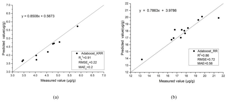
The grid search method was used in this study to find the best base regression, learning rate, loss function, and cycle number of the base regression. The search range and step size of each parameter in the grid search was initialized as follows: base estimators were RR, KRR, BRR, and a decision tree; value range of learning rate: 0.01–0.15, step size was set to 0.01; loss function: linear, square, and exponential; and value range of estimators: 50–300, step size was set to 50. The sample data was divided, the test error was calculated, five-fold cross-validation was selected, and after five training data iterations, the group parameter test results were selected as the mean values of the MSE. The optimal parameter combination was obtained from within the parameter range and the parameter combination was replaced. The average MSE value under all the parameter combinations in the grid was calculated successively. The parameter combination corresponding to the minimum MSE value was then obtained, which was the optimal parameter combination in the grid interval [27,28,29]. It can be seen from Table 4 that for the northwest China area, from the of the verification set, the maximum value of AdaBoost-KRR was 0.91, and the and of the validation set had the same trend. For the Honghu area, from the of the verification set, the maximum value of AdaBoost-RR was 0.86, and the and of the validation set had the same trend.
Table 4.
The results of the quantitative inversion models of soil organic matter.
| Study Area | Model | Learning Rate |
Loss Function | Estimators | |||
|---|---|---|---|---|---|---|---|
| Northwest China | AdaBoost-KRR | 0.05 | Square | 300 | 0.91 | 0.22 | 0.20 |
| Honghu | AdaBoost-RR | 1.0 | Linear | 50 | 0.86 | 0.72 | 0.56 |
Figure 7 compares the measured and predicted values of the different models. The x-axis shows the measured values of the SOM content and the y-axis shows the predicted values of the different models used for SOM content prediction. It can be seen that the overall accuracy of the models was high, and the relationship between the SOM content and measured hyperspectral reflectivity was well simulated.
Figure 7.
Comparison of the measured and predicted values of the different models:(a) northwest China and (b) Honghu.
4. Discussion
The correlation between an original reflectance and soil SOM content is not high. Different spectral transformations can enlarge and highlight the spectral characteristics of the original spectral reflectance and provide more characteristic bands on the original basis, which is conducive to the quantitative inversion of soil SOM content [24,30]. The correlation between spectral reflectance and soil SOM content can be effectively improved based on 10 spectral transformations, and the use of the higher correlation band can significantly improve the stability and prediction ability of the model [31].
In this study, an AdaBoost algorithm based on grid search optimization was introduced, and a variety of integrated learning soil organic matter quantitative inversion models were established. The prediction results of the AdaBoost algorithm based on grid search optimization and a single prediction model were compared and analyzed. From the results, the AdaBoost algorithm based on grid search optimization effectively improved the defect that a single prediction model has, namely that it easily falls into a local optimum. The results show that the algorithm effectively improved the prediction accuracy of the whole sample and the model generalization rate [29].
Compared with wide band remote sensing, hyperspectral remote sensing has the characteristics of high spectral resolution and strong band continuity. It can obtain more precise spectral information and is an important tool for the quantitative analysis of shallow soil properties. The spectral characteristics of soil spectral reflectance are caused by the mutual absorption and overlapping responses of different soil components. Estimations of specific soil attribute parameters can easily be affected by other soil components. Therefore, in this study, the combined spectral index model was used to focus on the mutual influence between bands, which can eliminate the mutual interference between band reflectance [32].
With the continuous progress of hyperspectral sensor technology, the difficulty of hyperspectral data acquisition is reduced. Therefore, the use of airborne or satellite hyperspectral sensors to obtain soil hyperspectral data has great potential for estimating regional soil surface organic matter content [33].
5. Conclusions
The general situations regarding the northwest China and Honghu study areas were as follows:
-
(1)
The data quality had a significant impact on the modeling effect. By comparing the original spectral data and the correlation coefficient between the data transformed by the different spectral indices and SOM, it was found that the correlation was greatly improved after treatment, and the correlation between SOM and the measured spectrum increased. It is therefore important to study how to remove redundant data and improve the data quality.
-
(2)
The regression ability of the ensemble learning algorithm was stronger than that of the traditional regression algorithm for the SOM spectrum. By using the AdaBoost algorithm based on a grid search, the prediction accuracy determination coefficient for the different regions could reach 0.85 or even higher. For the northwest China area, from the of the verification set, the maximum value of AdaBoost-KRR was 0.91, and for the Honghu area, from the of the verification set, the maximum value of AdaBoost-RR was 0.86, and the model had a better generalization ability.
-
(3)
The experimental results prove that the hyperspectral technique is feasible for the analysis of the SOM content of soil. The different spectral index transformations combined with the Pearson correlation analysis spectral feature selection method solves the problem of information redundancy and poor prediction accuracy in the spectrum inversion domain. The proposed method could also be applied to the monitoring and identification of other agricultural soils.
Acknowledgments
We gratefully acknowledge the help of the Data Extraction and Remote Sensing Analysis Group of Wuhan University (RSIDEA) in collecting the data. The Remote Sensing Monitoring and Evaluation of Ecological Intelligence Group of Hubei University (RSMEEI) helped to process the data.
Author Contributions
L.W. and Z.Y. were responsible for the overall design of the study and contributed to the proofreading of the manuscript. Z.Y. performed the experiments, analyzed and interpreted the data, wrote the manuscript, and helped with the proofreading of the manuscript. Z.W. and L.Z. contributed to designing the study and the proofreading of the manuscript. Y.Z., X.L., and L.C. analyzed and interpreted the data. All authors have read and agreed to the published version of the manuscript.
Funding
This research was funded by the National Key Research and Development Program of China (2019YFB2102902, 2017YFB0504202), the Open Fund of Key Laboratory of Urban Land Resources Monitoring and Simulation, MNR (KF-2019-04-006), the Opening Foundation of State Key Laboratory of Geo-Information Engineering (SKLGIE2018-M-3-3), the Central Government Guides Local Science and Technology Development Projects (2019ZYYD050), the Opening Foundation of Hunan Engineering and Research Center of Natural Resource Investigation and Monitoring (2020-2), the Open Fund of the State Laboratory of Information Engineering in Surveying, Mapping, and Remote Sensing, Wuhan University (18R02), and the Open Fund of Key Laboratory of Agricultural Remote Sensing of the Ministry of Agriculture (20170007).
Conflicts of Interest
The authors declare no conflicts of interest.
References
- 1.Parolo M.E., Savini M.C., Loewy R.M. Characterization of soil organic matter by FT-IR spectroscopy and its relationship with chlorpyrifos sorption. J. Environ. Manag. 2017;196:316–322. doi: 10.1016/j.jenvman.2017.03.018. [DOI] [PubMed] [Google Scholar]
- 2.Mcbratney A.B., Stockmann U., Angers D.A., Minasny B., Field D.J. Challenges for Soil Organic Carbon Research. Springer; Cham, Switzerland: 2014. pp. 3–16. [Google Scholar]
- 3.Ben-Dor E., Banin A. Near-Infrared Analysis as a Rapid Method to Simultaneously Evaluate Several Soil Properties. Soil Sci. Soc. Am. J. 1995;59:364. doi: 10.2136/sssaj1995.03615995005900020014x. [DOI] [Google Scholar]
- 4.Tan K., Ma W., Wu F., Du Q. Random forest–based estimation of heavy metal concentration in agricultural soils with hyperspectral sensor data. Environ. Monit. Assess. 2019;191:446. doi: 10.1007/s10661-019-7510-4. [DOI] [PubMed] [Google Scholar]
- 5.Gholizadeh A., Saberioon M., Bendor E., Borůvka L. Monitoring of selected soil contaminants using proximal and remote sensing techniques: Background, state-of-the-art and future perspectives. Crit. Rev. Environ. Sci. Technol. 2018;48:243–278. doi: 10.1080/10643389.2018.1447717. [DOI] [Google Scholar]
- 6.Nawar S., Buddenbaum H., Hill J., Kozak J., Mouazen A.M. Estimating the soil clay content and organic matter by means of different calibration methods of vis-NIR diffuse reflectance spectroscopy. Soil Till. Res. 2016;155:510–522. doi: 10.1016/j.still.2015.07.021. [DOI] [Google Scholar]
- 7.Steinberg A., Chabrillat S., Stevens A., Segl K., Foerster S. Prediction of Common Surface Soil Properties Based on Vis-NIR Airborne and Simulated EnMAP Imaging Spectroscopy Data: Prediction Accuracy and Influence of Spatial Resolution. Remote Sens. Basel. 2016;8:613. doi: 10.3390/rs8070613. [DOI] [Google Scholar]
- 8.Mcdonald G.C. Ridge regression. Wiley Interdiscip. Rev. Comput. Stat. 2010;1:93–100. doi: 10.1002/wics.14. [DOI] [Google Scholar]
- 9.Liu H., Miao E.M., Wei X.Y., Zhuang X.D. Robustness Modeling Method for Thermal Error of CNC Machine Tools Based on Ridge Regression Algorithm. Int. J. Mach. Tool Manu. 2017;113:S903489565. doi: 10.1016/j.ijmachtools.2016.11.001. [DOI] [Google Scholar]
- 10.Avron H., Clarkson K.L., Woodruff D.P. Faster Kernel Ridge Regression Using Sketching and Preconditioning. Siam J. Matrix Anal. Appl. 2017;38:1116–1138. doi: 10.1137/16M1105396. [DOI] [Google Scholar]
- 11.Shi Q., Abdel-Aty M., Lee J. A Bayesian ridge regression analysis of congestion’s impact on urban expressway safety. Accid. Anal. Prev. 2016;88:124–137. doi: 10.1016/j.aap.2015.12.001. [DOI] [PubMed] [Google Scholar]
- 12.Kalatzis A.E.G., Bassetto C.F., Azzoni C.R. Multicolinearity and Financial Constraint in Investment Decisions: A Bayesian Ridge Regression. J. Appl. Stat. 2008;38:287–299. doi: 10.1080/02664760903406462. [DOI] [Google Scholar]
- 13.Collins M., Schapire R.E., Singer Y. Logistic Regression, AdaBoost and Bregman Distances. Mach. Learn. 2002;48:253–285. doi: 10.1023/A:1013912006537. [DOI] [Google Scholar]
- 14.Wan J., Kang S., Tang C., Yan J., Ren Y., Liu J., Gao X., Banerjee A., Ellis L.B., Li T. Meta-prediction of phosphorylation sites with weighted voting and restricted grid search parameter selection. Nucleic Acids Res. 2008;36:e22. doi: 10.1093/nar/gkm848. [DOI] [PMC free article] [PubMed] [Google Scholar]
- 15.Chan J.C.W., Paelinckx D. Evaluation of Random Forest and Adaboost tree-based ensemble classification and spectral band selection for ecotope mapping using airborne hyperspectral imagery. Remote Sens. Environ. 2008;112:2999–3011. doi: 10.1016/j.rse.2008.02.011. [DOI] [Google Scholar]
- 16.Zhang X., Sun W., Cen Y., Zhang L., Wang N. Predicting cadmium concentration in soils using laboratory and field reflectance spectroscopy. Sci. Total Environ. 2019;650:321–334. doi: 10.1016/j.scitotenv.2018.08.442. [DOI] [PubMed] [Google Scholar]
- 17.Wei L., Yuan Z., Zhong Y., Yang L., Hu X., Zhang Y. An Improved Gradient Boosting Regression Tree Estimation Model for Soil Heavy Metal (Arsenic) Pollution Monitoring Using Hyperspectral Remote Sensing. Appl. Sci. 2019;9:1943. doi: 10.3390/app9091943. [DOI] [Google Scholar]
- 18.Sun W., Zhang X. Estimating soil zinc concentrations using reflectance spectroscopy. Int. J. Appl. Earth Obs. 2017;58:126–133. doi: 10.1016/j.jag.2017.01.013. [DOI] [Google Scholar]
- 19.Wang J., Cui L., Gao W., Shi T., Chen Y., Gao Y. Prediction of low heavy metal concentrations in agricultural soils using visible and near-infrared reflectance spectroscopy. Geoderma. 2014;216:1–9. doi: 10.1016/j.geoderma.2013.10.024. [DOI] [Google Scholar]
- 20.Liu Z., Lu Y., Peng Y., Zhao L., Wang G., Hu Y. Estimation of Soil Heavy Metal Content Using Hyperspectral Data. Remote Sens. Basel. 2019;11:1464. doi: 10.3390/rs11121464. [DOI] [Google Scholar]
- 21.Zhao L., Hu Y., Zhou W., Liu Z., Pan Y., Shi Z., Wang L., Wang G. Estimation Methods for Soil Mercury Content Using Hyperspectral Remote Sensing. Sustainability. 2018;10:2474. doi: 10.3390/su10072474. [DOI] [Google Scholar]
- 22.Galvão R.K., Araujo M.C., José G.E., Pontes M.J., Silva E.C., Saldanha T.C. A method for calibration and validation subset partitioning. Talanta. 2005;67:736–740. doi: 10.1016/j.talanta.2005.03.025. [DOI] [PubMed] [Google Scholar]
- 23.Wei L., Yuan Z., Yu M., Huang C., Cao L. Estimation of Arsenic Content in Soil Based on Laboratory and Field Reflectance Spectroscopy. Sensors. 2019;19:3904. doi: 10.3390/s19183904. [DOI] [PMC free article] [PubMed] [Google Scholar]
- 24.Wang S., Chen Y., Wang M., Zhao Y., Li J. SPA-Based Methods for the Quantitative Estimation of the Soil Salt Content in Saline-Alkali Land from Field Spectroscopy Data: A Case Study from the Yellow River Irrigation Regions. Remote Sens. Basel. 2019;11:967. doi: 10.3390/rs11080967. [DOI] [Google Scholar]
- 25.Alayet F., Mezned N., Sebai A., Abdeljaouad S. Continuum removed band depth analysis for carbonate mining waste quantification using X-ray diffraction and hyperspectral spectroscopy in the north of Tunisia. J. Appl. Remote Sens. 2017;11:16021. doi: 10.1117/1.JRS.11.016021. [DOI] [Google Scholar]
- 26.Dotto A.C., Dalmolin R.S.D., Grunwald S., Ten Caten A., Pereira Filho W. Two preprocessing techniques to reduce model covariables in soil property predictions by Vis-NIR spectroscopy. Soil Till. Res. 2017;172:59–68. doi: 10.1016/j.still.2017.05.008. [DOI] [Google Scholar]
- 27.Pillai N., Schwartz S.L., Ho T., Dokoumetzidis A., Bies R., Freedman I. Estimating parameters of nonlinear dynamic systems in pharmacology using chaos synchronization and grid search. J. Pharmacokinet. Phar. 2019;46:193–210. doi: 10.1007/s10928-019-09629-4. [DOI] [PMC free article] [PubMed] [Google Scholar]
- 28.Huang Q., Mao J., Yong L. In An improved grid search algorithm of SVR parameters optimization; Proceedings of the IEEE International Conference on Communication Technology; Chengdu, China. 9–11 November 2013. [Google Scholar]
- 29.Yang Y., Mei-Jing L.U. Classification method based on AdaBoost-SVM for wine quality. Comput. Eng. Des. 2017;9:44. [Google Scholar]
- 30.Tan K., Ye Y., Du P. Estimation of heavy-metals concentration in reclaimed mining soils using reflectance spectroscopy. Spectrosc. Spectr. Anal. 2014;34:3317–3322. [PubMed] [Google Scholar]
- 31.Liu J., Dong Z., Sun Z., Ma H., Shi L. Study on Hyperspectral Characteristics and Estimation Model of Soil Mercury Content. IOP Conf. Ser. Mater. Sci. Eng. 2017;274:12030. doi: 10.1088/1757-899X/274/1/012030. [DOI] [Google Scholar]
- 32.Hong Y.-S., Zhu Y.-X., Su X.-P., Zhu Q., Zhou Y., Yu L. Estimation of Soil Organic Matter Content Using Hyperspectral Techniques Combined with Normalized Difference Spectral Index. Spectrosc. Spectr. Anal. 2017;37:3537–3542. [Google Scholar]
- 33.Yu S., Yao Y., Wang D., Si H. Studies on the Inversion of Soil Organic Matter Content Based on Hyper-spectrum. Chin. Agric. Sci. Bull. 2013;29:146–152. [Google Scholar]


