Abstract
Pandemic influenza is a regularly recurring form of infectious disease; this work analyses its economic effects. Like many other infectious diseases influenza pandemics are usually of short, sharp duration. Human coronavirus is a less regularly recurring infectious disease. The human coronavirus pandemic of 2019 (COVID-19) has presented with seemingly high transmissibility and led to extraordinary socioeconomic disruption due to severe preventative measures by governments. To understand and compare these events, epidemiological and economic models are linked to capture the transmission of a pandemic from regional populations to regional economies and then across regional economies. In contrast to past pandemics, COVID-19 is likely to be of longer duration and more severe in its economic effects given the greater uncertainty surrounding its nature. The analysis indicates how economies are likely to be affected due to the risk-modifying behaviour in the form of preventative measures taken in response to the latest novel pandemic virus.
Keywords: Computable general equilibrium, Human coronavirus, COVID-19, Infectious diseases, Pandemic influenza, Periodicity, Trade linkages
Highlights
-
•
The dynamic effects of pandemic influenza and human coronavirus are analysed.
-
•
Epidemiological and economic models are linked to capture the transmission from regional populations to regional economies.
-
•
COVID-19 is likely to be of longer duration and more severe in its economic effects than previous pandemics.
-
•
The analysis indicates how economies are likely to be affected due to risk-mitigating preventative measures.
1. Introduction
Infectious diseases are a leading cause of death worldwide accounting for a quarter to a third of all mortality.1 Despite developments in pharmaceuticals infectious disease rates are rising due to changes in human behaviour, larger and denser cities, increased trade and travel, the inappropriate use of antibiotic drugs, and the emergence of new and resurgent pathogens [1]. The current outbreak of human coronavirus (COVID-19) is a reminder of the ease with which infectious disease outbreaks can cross borders and threaten economic stability. This has been observed before with similar outbreaks such as HIV, H1N1, H5N1 and SARS (e.g., Ref. [[2], [3], [4], [5], [6]]). The threat to stability derives from a number of features of these outbreaks.
One, by definition emerging diseases are not commonly encountered by physicians and are thus capable of generating widespread infection and mortality prior to identification of the etiologic agent (e.g., HIV/AIDS). COVID-19 has been especially challenging to contain because it is more contagious than influenza due to its ability to survive on surfaces and objects and transmit between people in this way [7]. Two, drug development and approval timeline lag well behind the emergence of these diseases such that the initial infection can result in significant mortality. Three, the constant adaptation of microbes, along with their ability to evolve and become resistant to antibacterial and antiviral agents, ensures that infectious diseases will remain a continuous and evolving threat.
Pandemic influenza is a regularly recurring form of infectious disease. It is possible that the current outbreak of human coronavirus may also become a regularly recurring form of infectious disease given it represents the second strain of severe acute respiratory syndrome coronavirus (SARS-CoV-2) — the first strain led to the outbreak of SARS (SARS-CoV-1) during 2002–2003 [8]. This work assesses the economic effects of such infectious diseases with a focus on the dynamic effects. This is done by initially analysing a hypothetical influenza pandemic with characteristics consistent with previous historical occurrences; subsequently a pandemic that mimics some of the known (at this point) characteristics of the COVID-19 pandemic is analysed.
There are a number of previous studies analysing the economic effects of global pandemics. A general equilibrium approach is the ideal framework for properly evaluating the economic impacts of public health emergencies such as pandemic influenza and human coronavirus. A partial equilibrium approach that only focuses on the health sector and forgone incomes resulting from disease-related morbidity and mortality, while ignoring effects in other parts of the economy (e.g. Ref. [9]), is incomplete. Illness and death due to public health emergencies raise perceptions of risk, leading to risk-modifying behaviour (such as prophylactic absenteeism from work and public gatherings) in an effort to reduce the risk of contracting illness. Risk-modifying behaviour affects consumption and reduces labour productivity. Deaths due to illness reduce the supply of workers. The effects of risk-modifying behaviour and deaths will affect all parts of the economy to a greater or lesser extent.
An important feature of pandemics is their short, sharp nature; they usually begin and end within a year. Previous studies focusing on the economic effects of global pandemics apply either a macroeconomic or computable general equilibrium (CGE) approach. Although macroeconomic (i.e., single sector) approaches (e.g. Ref. [5]), have the advantage of applying quarterly models that allow them to capture the short, sharp nature of pandemics; they have the disadvantage of a single-sector approach that ignores sectors that are particularly relevant to the study of the economic effects of epidemics (e.g., medical services, international tourism). Although CGE (i.e., multi-sector) approaches (i.e. [2]), apply models that have the advantage of identifying multiple sectors in the economy, they have the disadvantage of annual periodicity and so are unable to capture accurately the short, sharp nature of influenza pandemics. The disadvantage of the CGE approach has been addressed by studies applying CGE models with quarterly periodicity, e.g., Ref. [6]. The same approach is taken here.
The results show that pandemics can cause large short-term effects on output with small ongoing longer-term effects. The two main drivers of the contractions in output are the fall in international and domestic travel and tourism and reduced labour productivity, the latter being more important when severe mitigation measures are adopted by governments such as during the current coronavirus pandemic.
2. The nature of influenza pandemics
2.1. Overview
Influenza is a contagious disease that causes seasonal epidemics globally and is a leading cause of infectious disease-related deaths in most countries. Influenza mortality is highly variable from year to year and is a contributor to the variability in the annual mortality rate of industrialised countries. In non-pandemic years, influenza typically kills hundreds of thousands of people worldwide. Occasionally, influenza rates can reach pandemic proportions. There have been four influenza pandemics since the beginning of the 20th century — 1918, 1957, 1968 and 2009 — each of which was the result of a major genetic change to the virus.
Of these four influenza pandemics the most severe was the 1918 Spanish Flu pandemic where influenza mortality reached as high as 35 times the yearly average. More recently, May 2009 saw the emergence from Mexico of a new H1N1 virus capable of human-to-human transmission. The 2009 H1N1 virus was a novel type of influenza A that was highly transmissible yet ultimately mild. It quickly spread around the world infecting 74 different countries in all six continents within five weeks. The rate of spread was far more rapid than previously observed and was enabled by high volumes of international air traffic. The World Health Organization declared a pandemic on June 11, 2009. Thus, the virus took less than two months to emerge from Mexico and travel to all parts of the globe. It ultimately reached more than 200 countries and infected hundreds of millions of people. The World Health Organization declared the pandemic over by the end of the year reflecting the brief lifespan of such viruses.
The current human coronavirus pandemic (COVID-19) began in December 2019 in China and was caused by a novel virus (SARS-CoV-2) that is the second strain of severe acute respiratory syndrome coronavirus; the first strain led to the outbreak of SARS (SARS-CoV-1) in East Asia during 2002–2003 [8]. The current coronavirus outbreak was declared a pandemic in March 2020 [10] and is currently in play. As of April 29, 2020 there are 3.1 million confirmed cases in 185 countries, 217,000 deaths and 935,000 recovered cases [11]. The virus is thought to spread primarily through person-to-person contact via droplets produced when an infected person coughs, sneezes or talks. Infection may also occur via contact with contaminated surfaces and objects; this is a novel transmission compared to influenza-type viruses [7].
One important metric of an infectious disease outbreak is the case fatality rate (CFR): the ratio of total deaths to total cases. The COVID-19 outbreak is still in play and until it ends it is difficult to provide a proper comparison to previous global outbreaks. For instance, Ref. [12] estimate a CFR prediction interval for COVID-19 of 0.82%–9.64% as at the end of April 2020. They note “Evaluating CFR during a pandemic is, however, a very hazardous exercise, and high-end estimates should be treated with caution as the H1N1 pandemic highlights that original estimates were out by a factor greater than 10.” This is explained by Ref. [13] “A major challenge with accurate calculation of the CFR is the denominator” (p. 1), which is affected by asymptomatic cases, cases with mild symptoms, or misdiagnosed cases; thus under- and over-estimating the CFR. Their assessment is that despite its high transmissibility the coronavirus CFR appears lower than SARS (9.5%) but higher than seasonal influenza (0.1%) and H1N1 (0.1%).2 This would be consistent with the current lower-bound prediction of 0.82% of [12].
In socio-economic terms the defining features of COVID-19 are (i) the almost complete global spread of the virus within four months, and (ii) the extensive socioeconomic disruption due to preventative measures taken by governments. An example of unprecedented preventative measures is the almost total shutdown of domestic and international travel due to internal and external border closures [14].
2.2. The effect on human behaviour
Direct economic effects of illness resulting from influenza include increased healthcare expenditures and workloads. Indirect effects include a permanently smaller labour supply due to deaths, and increased absenteeism from work by sick workers and by workers wishing to reduce the risk of contracting illness in the workplace, i.e., prophylactic absenteeism.
Prophylactic absenteeism is one example of voluntary risk-modifying behaviour in response to a pandemic. Other examples are reduced domestic and international travel, and reduced public gatherings at sporting and other events. Non-voluntary risk-modifying behaviour may be imposed on workers with children by school closures intended to mitigate the spread of the virus [15]. Thus, some workers will be forced to take leave to care for young children. Workers who take paid leave from work, whether forced or voluntary, reduce their firm's labour productivity (i.e., output per worker) unless other workers can fully replace output lost due to absenteeism. This may be difficult during an influenza pandemic because the virus will be widespread and while many workers may not present to the health system they are likely to be less productive than would otherwise be the case.
[3] argues that a pandemic will reduce business investment due to increased uncertainty and risk, leading to excess capacity. Similarly, consumer confidence will decline due to uncertainty and fear, leading to reduced spending as people elect to be homebound to reduce the probability of infection—this is another example of risk-modifying behaviour. Reduced consumer confidence may particularly affect services involving face-to-face contact (e.g., tourism, transportation and retail spending). [16] argue that evidence from past pandemics suggests that it is mainly discretionary spending (e.g., tourism and transportation) that is reduced.
[3] argues that an epidemic does not need to be of high morbidity and mortality in order to exert a large psychological impact on attitudes to risk. e.g., the 2003 SARS epidemic. [16] examine evidence from the SARS epidemic and argue that the only economic impact was on air travel to affected locations and related impacts on accommodation. [17] perform a retrospective analysis of the economic impact of the 2003 SARS epidemic and find that the economic effects were mainly but not exclusively centred on East Asian regions, and that the effects went beyond air travel and accommodation.
The response by individuals and governments to coronavirus supports the argument made above by Ref. [3]. It is likely (but not certain) that the ultimate coronavirus CFR will be much lower than SARS but higher than seasonal influenza. Despite this, the socio-economic disruption of coronavirus is disproportional to its morbidity and mortality. The mitigation measures taken to contain the virus are expected to lead to a significant global contraction in the order of 3% for 2020 [18].
3. The economic model
To model the economic consequences of infectious disease outbreaks a global CGE model is applied. A formal presentation of the model is available in Ref. [19]; a largely descriptive presentation is presented below.
The model represents the world economy as multiple regions engaging in trade and investment: markets are perfectly competitive, industry technologies are linearly homogeneous, and traded goods are imperfectly substitutable. Formally, the model is represented in homogeneous form by nonlinear equations specifying behavioural and definitional relationships as
| (1) |
where Fi are i (=1, …,m) continuous and differentiable functions, N is a vector of endogenous variables and X is a vector of exogenous variables. Typically, X describes changes in economic structure and policy (e.g., tax rates, labour productivity) and can be used to perturb the model to simulate changes in N.3
3.1. Intratemporal theory
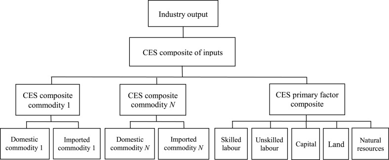
The model represents the world economy as economic activity occurring within and across regional economies. A regional economy may be either a single country (e.g., France) or a country group (e.g., the European Union). Each region produces a distinct variety of each commodity that is imperfectly substitutable with the varieties produced by other regions. Each regional commodity is produced from inputs of domestically-produced and imported commodities and five primary factors: skilled and unskilled labour, capital, land and natural resources (see Fig. 1 ).
Fig. 1.
Structure of industry production technology.
Labour and capital are perfectly mobile across industries within a region whereas land and natural resources are fixed in industry usage. Consequently, wages for each labour type and the user price of capital are uniform across industries but the rental prices of land and natural resources can vary across industries.
Regional commodities can be consumed as inputs to final demand of which there are four categories: investment, government consumption, household consumption and exports. Exports aside, final demands use composite commodities that are constant elasticity of substitution (CES) combinations of the domestic and the imported variety of each commodity, similar to composite commodity inputs for industries (Fig. 1). Composite commodity inputs to investment and government consumption are determined by CES production and utility functions, while household consumption is determined by a constant-differences-elasticity utility function. A Cobb-Douglas utility function with variable scale and share parameters determines the allocation of regional income across government consumption, household consumption and saving. The model is calibrated using the GTAP database [20] aggregated to 27 regions and 30 sectors (see Table 1 ).
Table 1.
Regions and sectors in model database.
| Region | Sector |
|---|---|
| 1. Australia | 1. Agriculture |
| 2. Rest of Oceania | 2. Coal |
| 3. China | 3. Oil |
| 4. Japan | 4. Gas |
| 5. Korea | 5. Other minerals |
| 6. India | 6. Processed food |
| 7. Indonesia | 7. Beverages and tobacco products |
| 8. Singapore | 8. Textiles, wearing apparel |
| 9. Rest of Asia | 9. Leather, wood products |
| 10. Canada | 10. Paper products, publishing |
| 11. United States of America | 11. Petroleum, coal products |
| 12. Mexico | 12. Chemicals, rubber, plastics |
| 13. Argentina | 13. Other mineral products |
| 14. Brazil | 14. Metals, metal products |
| 15. Rest of South & Central America, Caribbean | 15. Motor vehicles and parts |
| 16. France | 16. Other transport equipment |
| 17. Germany | 17. Electronic equipment |
| 18. Italy | 18. Other manufacturing |
| 19. Great Britain | 19. Utilities |
| 20. Rest of European Union | 20. Construction |
| 21. Rest of Europe | 21. Wholesale & retail trade |
| 22. Russia | 22. Air transport |
| 23. Former Soviet Union | 23. Other transport |
| 24. Turkey | 24. Communication |
| 25. Rest of Middle East, North Africa | 25. Other financial services |
| 26. South Africa | 26. Insurance |
| 27. Rest of Sub-Saharan Africa | 27. Other business services |
| 28. Recreation, other services | |
| 29. Government services | |
| 30. Dwellings |
As mentioned above, the model can be used to observe changes in endogenous variables due to changes in exogenous variables. Thus changes in tax rates and labour productivity can be applied on a region-specific or industry-specific basis and the model will project changes in industry output, prices, international trade, household consumption and GDP, among other variables. The dynamic aspects of the model are described below. This means that the time path of changes in endogenous variables can also be observed. The responses projected by the model reflect a perturbation of the initial steady state with a given capital-labour ratio to a new steady state once a new capital-labour ratio is reached.
3.2. Annual and quarterly dynamics
Annual models are well suited to analysing events that last for about a year or more. But for events that have short and sharp effects, such as infectious disease outbreaks, a quarterly model is more appropriate as an annual model will smooth short-term effects leading to potential underestimation of disruption. For example, if a pandemic caused an 80% loss of inbound international tourism within a particular quarter, then the adjustment path of the tourism industry would be quite different from a situation in which international tourism declined smoothly by 20% for a year.
Annual CGE models are commonly solved in recursive fashion.4 Recursive or sequenced dynamic models usually divide time into discrete intervals and economic variables are assumed to change at the end of each interval. Such models take the form
| (2) |
where N and X are vectors of endogenous and exogenous variables in a period, and Gi(i = 1, …,m) are m differentiable and continuous functions. Computations can then be carried out according to
| (3) |
where refers to changes from one period to the next and is the vector of first-order partial derivatives of Gi.
Calibration of (3) requires an initial solution (i.e., a database consistent with the equations in (3)) mainly representing annual flows (e.g., household consumption, exports, etc.) and a choice of parameter values (e.g., price and income elasticities). To apply (3) as a quarterly model there are two options. One option is to modify the initial solution to (3) (i.e., the database) to represent quarterly rather than annual flows (i.e., divide annual flows by four).5 Another option is to leave the initial solution unchanged and modify (3) so that represents quarterly changes in exogenous variables, e.g., population growth. The simplest way to do this is to divide by four thus assuming constant quarterly changes through the year. This second option also requires the addition of equations that handle quarterly accumulation of stock variables; this can be done by again assuming constant quarterly changes through the year. With both options N will represent quarterly rather than annual endogenous variables.
3.3. Capital accumulation and investment
In a dynamic framework, capital accumulation is handled by a stock-flow equation linking capital stocks across periods that allows for investment (i.e., new capital) and depreciation of existing capital at a geometric rate:
| (4) |
where is the quantity of capital available for use in region r in year t, is the quantity of new capital created (i.e., investment) in region r during year t, and is depreciation of existing capital in region r. With and representing annual values, in (4) will grow at an annual rate. The model contains a second stock-flow relationship that treats accumulation on a quarterly basis:
| (5) |
In deriving (5), quarterly values for depreciation, , and investment, , are applied that ensure accumulates at a quarterly rate. That is, and . The relevant equation for any given simulation depends on whether annual or quarterly dynamics are applied.
The investment-capital ratio, , in each region is assumed to be a positive function of the rate of return. This relationship is calibrated to reflect increasing (convex) costs of adjusting the capital stock by larger amounts. This treatment captures the inertia in investment behaviour as observed in empirical studies.6
3.4. The labour market
The supply of each labour type is assumed to be sensitive to the real wage consistent with international evidence on non-zero wage elasticities of labour supply (e.g. Ref. [21],:
| (6) |
Thus the supply of labour type l in region r in year t, , as a share of population in year t, , is determined as a function of the real post-tax wage received by labour type l in region r in year t, . and β are positive constants. With the uncompensated labour supply elasticity β = 0.15, labour supply is only slightly responsive to the real return to labour in each region. Note that a similar relationship to (6) applies in the quarterly model.
Employment by labour type is an endogenous function of slowly-adjusting wage rates. In the short-run, wage rates grow at the rate of inflation from period to period in the absence of labour market shocks. Where the market is in disequilibrium (i.e., the unemployment rate deviates from its long-run value) wage rates will grow more (less) quickly than the inflation rate if the unemployment rate is falling (rising). Hence, the rate of wage adjustment per period depends on labour market conditions relative to the long-run unemployment rate. This is consistent with empirical evidence that the rate of wage adjustment is partially determined by non-Walrasian features of the economy (see Ref. [22]; chapter 9).
3.5. Generating model results
The baseline path of the model begins from an observed equilibrium (2004) that evolves to a balanced growth path. The starting data are updated from 2004 to 2009 by incorporating historical movements in real GDP and labour supply.7 From 2010 to 2025 historical population movements are applied, and 2% annual growth in labour productivity and fixed factors (land and natural resources) is assumed in all regions. Although the initial data do not represent a steady state, the assumptions for growth in labour productivity and fixed factors mean that the growth rate for all quantity variables converges close to the long-run growth rate for each region: population growth plus the growth in labour productivity.
4. The infectious disease model
The morbidity and mortality impact of the pandemic on the age cohorts of the population are taken from Ref. [23] who model them using a variation on the classic Susceptible-Exposed-Infected-Recovered (SEIR) model of infectious disease transmission. The SEIR model computes the theoretical number of people infected with an infectious disease in a closed population over time. This type of modelling is applicable to diseases where an individual that has recovered from the disease is removed from the susceptible population. In order to derive the equations of the model, the population of a single region or demographic group is divided into eight subpopulations: susceptible, vaccinated, exposed, three subsets of infected (untreated, hospitalised, and treated), recovered, and dead. Fig. 2 displays the way the model replicates the dynamics of a pandemic.
Fig. 2.
The SEIR model.
The susceptible population is decreased through vaccination and exposure to the virus; conversely, it is increased by the loss of vaccine-acquired immunity. Vaccinated individuals are not considered to be completely protected but become exposed at a rate much lower than the susceptible population. Vaccine efficacy can vary over the course of the epidemic. Typically, around one month is required after vaccination until the individual has produced sufficient antibodies for the vaccine to be effective. Even after this initial time period, vaccine efficacy will be less than 100% due to varying individual antibody response to vaccine and the possibility of viral mutation or an imperfectly-matched vaccine.
After exposure, individuals progress to one of three infected states: untreated, treated, and hospitalised. The proportion of individuals progressing into each category is dependent on viral characteristics. As the virulence of the virus increases, the proportion of the infected receiving treatment also increases. The duration of infectiousness and transmission probabilities are decreased for those receiving treatment. Through this mechanism the parameters of the model allow for the simulation of behavioural and medical quarantine.
An increase in virulence can result in a reduction of average transmissibility; individuals with a severe virus tend to be too ill to be out in the community transmitting the virus. In addition, those receiving treatment or who are hospitalised will have reduced contact and transmissibility due to precautionary measures such as masks, gloves, and isolation. Individuals remain infectious during the entire course of their clinical infection. Once they have progressed out of the infectious state they can no longer transmit the virus to others.
After infection, individuals progress to one of two groups: recovered or dead. The rate at which individuals progress from one of the three infected states (hospitalised, treated, or untreated) to the end states is dependent on virulence and the level of treatment during infection. Hospitalised individuals have the highest death rate, followed by treated and untreated cases. Many of the untreated individuals are likely to have subclinical or asymptomatic infections, which reduces death rates despite the fact that some with untreated clinical infections may be more likely to die.
Those individuals progressing to the recovered state are considered to have immunity for the duration of the pandemic. Pandemics tend to come in waves and infect geographic areas for short periods of time. It is unlikely that in the case of an influenza pandemic the strain will mutate enough to cause re-infection during a single pandemic wave. There are five morbidity states included in the model:
-
1
subclinical, where the infected person seeks no medical attention but purchases pharmaceuticals;
-
2
physician and flu clinic, where the infected person seeks medical attention by visiting a physician or a flu clinic;
-
3
hospitalisation, where the infected person is hospitalised and survives;
-
4
intensive care unit (ICU), where the infected person is hospitalised and spends time in an ICU and survives; and
-
5
death, where the infected person is hospitalised and dies.
5. The pandemic scenarios
5.1. The influenza pandemic
The influenza pandemic applied here begins in Vietnam and has a global fatality impact of around 0.01%. It is an extremely transmissible influenza virus with a global attack rate of approximately 40% despite the availability of an effective vaccine within months of the outbreak. The case fatality rate is 0.5%, which is similar to the 1957 influenza pandemic. Unlike seasonal influenza where typically 90% of the fatalities are observed in individuals older than 65, this virus has an equal case fatality across ages consistent with the 2009 H1N1 pandemic. The majority of cases are subclinical or physician visits and approximately one-fifth of those hospitalised require intensive care, analogous to what is observed in seasonal outbreaks.
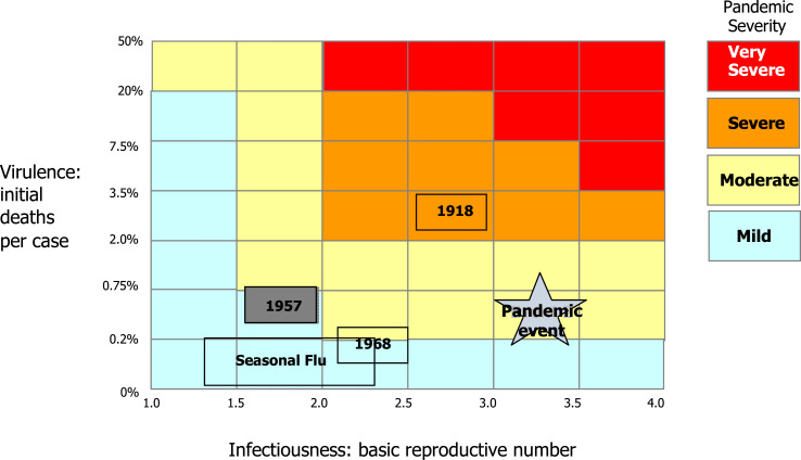
The pandemic scenario has viral characteristics that are plausible but less extreme than historical events, such as the 1918 pandemic. Fig. 3 shows how the pathogen characteristics of the scenario compares to historical flu pandemics. Epidemic curves were created for each country or region using the calculated correlation between the observed 2009 H1N1 pandemic transmission timeline and country density. A log-linear relationship between population and weeks until pandemic peak represented the most appropriate statistical fit. The epidemic curves were used to develop weekly totals of individuals in each of the five morbidity classes by country or region.
Fig. 3.
Pathogen characteristics of the modelled pandemic relative to historical pandemics.
Notes: Virulence is measured in terms of the case-fatality rate or deaths per infected case. Infectiousness (or transmissibility) represents the speed at which a pandemic will spread within a population and the total number of people that will be infected. Infectiousness of influenza is measured by the basic reproductive rate (R0), or the mean number of secondary cases an infectious case will cause in a population without immunity and without intervention. R0 > 1 is necessary for an epidemic to occur.
5.1.1. Morbidity and mortality
The SEIR model provides estimates of the number of persons newly infected per week and the severity of their infection in each region over the course of the year. Overall infection rates are high relative to previous pandemics: see the x-axis in Fig. 3. Further, infection rates are higher in lower income countries than in higher income countries, and higher in Asian regions, where the pandemic is assumed to begin, than in non-Asian regions.
The distribution of infected cases is skewed towards less severe cases and only a small proportion of infections result in death (0.5%). In historical terms, the pandemic's virulence (i.e., initial deaths per case) is similar to previous pandemics as shown on the y-axis in Fig. 3. Therefore, the majority of cases remain at the subclinical and physician/flu clinic levels of contact with the health system.
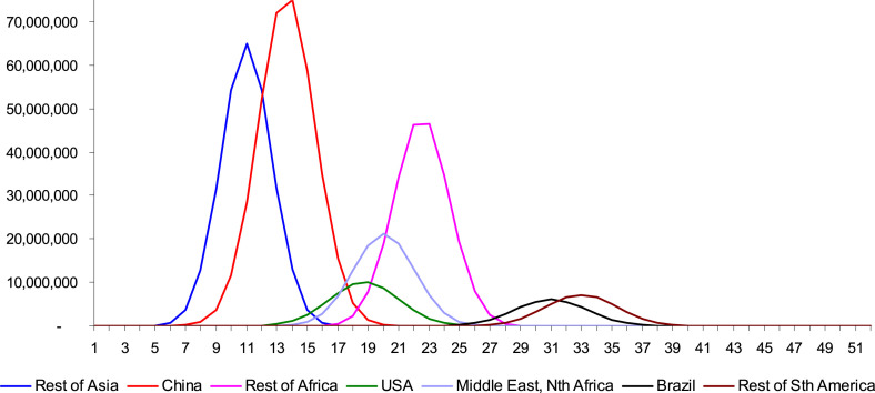
Fig. 4 presents a picture of the dynamics of the influenza outbreak; it is typical of historical influenza pandemics. Globally, new infections occur over about two-thirds (about 35 weeks) of the year. New infections peak around week 16, and there are two further smaller peaks around weeks 22 and 32. The pattern of new global infections partially obscures the short, sharp nature of the outbreak at the regional level. Fig. 4 shows that new infections last for only around 10 weeks in each region, on average. It also shows how the outbreak moves from continent to continent depending on international travel patterns. Thus, the outbreak begins in the Rest of Asia (Vietnam), moves quickly to China, then the United States and Africa, and lastly to South America. These dynamics are important in determining the timing of the economic effects across regions. The economic aspects of the outbreak's dynamics can not be captured by an economic model that does not also reflect these dynamics, i.e., periodicity of much less than one year.
Fig. 4.
New infections per week in selected regional populations - pandemic influenza scenario.
5.1.2. Direct economic effects
Previous analysis of influenza outbreaks and their potential economic effects highlights a number of channels through which an economy might be affected by a serious outbreak of influenza.8 These channels include: reduced consumption by households of tourism, transportation and retail trade; increased absence from the workplace due to illness or for prophylaxis; school closures; and higher demands for medical services. Considering these channels, four types of economic shocks are applied to simulate the influenza pandemic.
-
1.
A temporary surge in demand for hospital and other medical services. Increased medical spending related to each pandemic is applied as increased expenditure on the Government services sector.
-
2.
A temporary upsurge in sick leave and school closures. This represents workers falling ill and parents caring for children. These effects are modelled as a temporary decrease in output per worker (labour productivity).
-
3.
Deaths with a related permanent reduction in the labour force.
-
4.
Temporary reductions in international tourism and business travel. These are a function of the number of persons infected and the initial deaths per case. The shocks to tourism are applied to exports of four sectors: Wholesale and retail trade, Air transport, Other transport, and Recreation and other services. Such purchases represent spending by tourists.9
Note that with government consumption rising and household consumption falling, the national saving rate is not constant and may rise or fall depending on the relative changes in government and household consumption rates. Furthermore, the government budget is not held fixed in any period of the scenario.
5.2. The human coronavirus pandemic
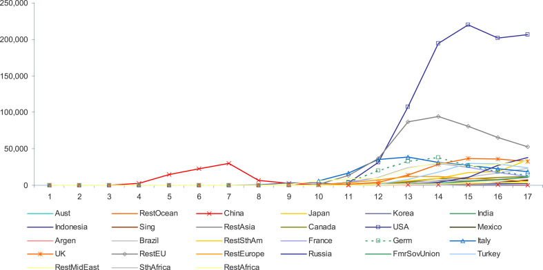
Using the influenza scenario described above as a benchmark, a scenario is fashioned to represent what is known about the human coronavirus pandemic as at the end of April 2020. Using data from Ref. [24] the spread of new infections is calculated from China in December 2019 to other countries over the 17 week period ending April 29, 2020; these data are presented in Fig. 5 . The data show that by week 9 four major countries and regions showed new weekly infections of greater than 1,000: China, Japan, Italy and Middle East-North Africa. By week 11 another six more major countries and regions had 1,000 or more new weekly infections: the United States, France, Germany, the United Kingdom, Other European Union countries, and Other European countries. By week 14 all other major countries and regions were recording 1,000 or more new weekly infections: Oceania by week 12, Brazil by week 12, Other South and Central American countries by week 12, Russia by week 13, India by week 14, Mexico by week 14, and Indonesia by week 15. Argentina is the only G20 country that did not reach 1,000 or more new weekly infections by week 17.
Fig. 5.
New infections per week by region - coronavirus.
For many of the countries and regions already discussed the rate of new weekly infections have already peaked and are now falling (as at end of April 2020. Those still showing a rising rate of new weekly infections are India, Singapore, Other Asian countries, Canada, the United States, Mexico, Brazil, Other South and Central American countries, Russia, Other former Soviet Union countries, Middle East-North Africa, South Africa and Other sub-Saharan African countries.
In the absence of further data, assumptions are applied to project the path of new infections from week 18 onwards. This is done by assuming a 5% weekly geometric rate of decay. This gives a path of new infections until week 52 that varies by country and country group. The direct effects of the coronavirus pandemic are then calculated as a function of the country-specific path of new infections through the year.
5.2.1. Direct economic effects
Using the data discussed above, direct economic effects qualitatively similar to the influenza scenario are designed so that regions whose rate of new infections have peaked start to ease mitigation measures in quarter 3, 2020. In contrast, regions whose rate of new infections are yet to peak start to ease mitigation measures in quarter 4, 2020: this assumes that the rate of new infections in these regions peaks by July 2020. These assumptions are not intended as predictions or probable. They only serve to provide a temporal boundary around the epidemiological characteristics of the outbreak, which in turn allows the analysis of the possible economic impacts of the pandemic. Six types of economic shocks are applied to simulate the coronavirus pandemic.
-
1.
A temporary surge in demand for hospital and other medical services. This effect is scaled to reflect the number of coronavirus infections relative to the number of pandemic influenza infections. Note that the number of coronavirus infections (as at the end of April 2020) are much lower than the number of pandemic influenza infections. This can be seen by comparing the scales in Fig. 4, Fig. 5.
-
2.
A temporary surge in demand for policing and related services. This effect is related to the enforcement of wide-ranging and compulsory social distancing measures imposed almost universally.10 It is assumed that this effect peaks at 5% of baseline government expenditures for all countries except Sweden and Singapore. The peak increase in spending coincides with the peak quarter of infections and then falls as new infections decline during the year.
-
3.
A temporary upsurge in sick leave, school and university closures, workplace closures and cancelled public events and gatherings. These effects are designed to reflect the wide range of severe mitigation measures that countries have undertaken to enforce compulsory social distancing in efforts to contain the spread of coronavirus.11 These effects focus on the impact on workplaces. It is assumed that this effect peaks at −20% of baseline economywide labour productivity for all countries except Sweden and Singapore. For Sweden and Singapore the peak is assumed to be −5%. The peak fall in labour productivity coincides with the peak quarter of infections and then falls as new infections decline during the year.
-
4.
Deaths with a related permanent reduction in the labour force. Similar to the point made in (1) above regarding infections, the number of coronavirus deaths (as at the end of April 2020) are much lower than the number of pandemic influenza infections.
-
5.
Temporary reductions in domestic and international tourism and business travel. During the initial stages of the outbreak there was a fall in international travel and tourism related to uncertainty surrounding the epidemiological characteristics of the virus and the cancellation of international gatherings. Eventually most countries closed their borders to all visitors and only allowed the entry of returning citizens and residents.12 This has led to the almost total shutdown of international travel and tourism. This is imposed as global reductions in the relevant sectors of 25%–60%. It is assumed that this peak effect is timed to coincide with the number of coronavirus infections through the year.
-
6.
Temporary switching of household and business expenditure away from domestic tourism and travel, restaurants and accommodation, sporting events and in-store retail purchases. The severe mitigation measures led to restrictions in a range of activities where person-to-person contact is typical; this affected restaurants and accommodation, sporting events and in-store retail purchases of non-essential goods. In most countries the mitigation measures also severely restricted inter- and intra-city movement, thus severely affecting domestic tourism and travel. The switching of expenditure away from these commodities is imposed as a 50% reduction in domestic sales in the relevant sectors. This peak effect is timed to coincide with the number of coronavirus infections through the year.
6. The economic effects of pandemic influenza
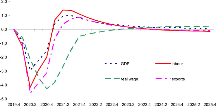
In this section we apply the direct effects of the pandemic to the economic model. Fig. 6 reports the effects on the levels of selected global variables relative to baseline; Table 2 reports the real GDP effects for all regions.
Fig. 6.
Global effects (percentage change).
Table 2.
Quarterly model effects: global and regional GDP (percentage change).
| Region |
Quarter |
|||||||
|---|---|---|---|---|---|---|---|---|
| 2020:1 | 2020:2 | 2020:3 | 2020:4 | 2021:1 | 2021:2 | 2021:3 | 2021:4 | |
| World | −0.80 | −2.97 | −2.23 | −1.54 | 0.39 | 0.96 | 0.98 | 0.81 |
| Australia | −0.57 | −2.51 | −2.03 | −1.38 | 0.41 | 0.98 | 1.00 | 0.77 |
| Rest of Oceania | −0.54 | −2.27 | −1.85 | −1.35 | 0.26 | 0.82 | 0.82 | 0.73 |
| China | −1.51 | −5.68 | −4.58 | −3.59 | 0.36 | 1.95 | 2.18 | 1.79 |
| Japan | −0.84 | −2.59 | −1.90 | −1.21 | 0.53 | 0.99 | 0.96 | 0.75 |
| Korea | −1.13 | −3.62 | −2.83 | −2.00 | 0.27 | 1.16 | 1.39 | 1.26 |
| India | −0.09 | −0.74 | −0.56 | −0.31 | 0.31 | 0.42 | 0.41 | 0.35 |
| Indonesia | −0.70 | −2.50 | −1.94 | −1.41 | 0.25 | 0.93 | 1.10 | 1.02 |
| Singapore | −2.40 | −7.35 | −5.84 | −4.52 | −0.31 | 1.84 | 2.60 | 2.53 |
| Rest of Asia | −0.65 | −3.22 | −2.53 | −1.87 | 0.02 | 0.66 | 0.95 | 0.85 |
| Canada | −0.76 | −3.19 | −2.33 | −1.69 | 0.42 | 1.07 | 0.99 | 0.79 |
| United States | −0.52 | −1.86 | −1.24 | −0.64 | 0.48 | 0.52 | 0.40 | 0.32 |
| Mexico | −0.08 | −0.50 | −0.31 | −0.15 | 0.23 | 0.37 | 0.37 | 0.34 |
| Argentina | −0.57 | −2.24 | −1.75 | −1.25 | 0.12 | 0.63 | 0.75 | 0.62 |
| Brazil | −0.25 | −1.07 | −0.71 | −0.50 | 0.28 | 0.50 | 0.47 | 0.45 |
| Rest of South America | −0.42 | −1.99 | −1.49 | −1.04 | 0.30 | 0.69 | 0.71 | 0.56 |
| France | −1.01 | −3.83 | −2.78 | −1.91 | 0.60 | 1.30 | 1.25 | 0.96 |
| Germany | −1.06 | −3.92 | −2.85 | −1.96 | 0.50 | 1.26 | 1.29 | 1.04 |
| Italy | −0.54 | −2.21 | −1.73 | −1.26 | 0.23 | 0.70 | 0.77 | 0.64 |
| Great Britain | −1.21 | −4.40 | −3.28 | −2.29 | 0.63 | 1.52 | 1.49 | 1.16 |
| Rest of EU | −1.38 | −5.07 | −4.06 | −3.16 | 0.13 | 1.46 | 1.70 | 1.41 |
| Rest Europe | −0.84 | −3.07 | −2.26 | −1.50 | 0.39 | 0.96 | 1.07 | 0.92 |
| Russia | −0.46 | −2.05 | −1.71 | −1.31 | 0.05 | 0.65 | 0.89 | 0.90 |
| Former Soviet Union | −0.60 | −2.68 | −2.18 | −1.62 | 0.10 | 0.70 | 0.84 | 0.75 |
| Turkey | −0.10 | −0.74 | −0.59 | −0.38 | 0.04 | 0.16 | 0.27 | 0.30 |
| Rest of Middle East | −0.26 | −1.45 | −1.08 | −0.71 | 0.31 | 0.55 | 0.55 | 0.51 |
| South Africa | −0.51 | −2.13 | −1.56 | −1.12 | 0.26 | 0.71 | 0.70 | 0.60 |
| Rest of Africa | −0.41 | −2.37 | −1.87 | −1.48 | 0.13 | 0.67 | 0.65 | 0.52 |
The main impacts occur in 2020, the pandemic year. In quarter 1 of 2020 (2020:1) the pandemic causes global GDP to fall by 0.8% and labour by 1.2%. In 2020:2, GDP and labour fall further (−3% and −4.2%) as new infections continue to rise (see Fig. 4). As new infections peak in 2020:2, so too do the negative effects on GDP and labour. The movements in GDP are mostly driven by movements in labour. Labour is the only variable input in the short-run as capital stocks are subject to a one-period gestation lag and take time to respond to the pandemic. The contractionary effect of the pandemic reduces demand for labour by firms. As wage rates are rigid in the short-run they do not fall enough to maintain labour usage, thus causing the fall in labour to be greater than would otherwise be case.
In 2020:3 the number of new global infections falls significantly as there are no new infections in Asia (the origin of the virus) and Europe; in 2020:4 there are only a small number of new infections and these are in Australia and South America. Although there are few new infections in 2020:3 and 2020:4, the pandemic keeps global economic activity depressed due to continuing precautionary measures (e.g., voluntary and compulsory restrictions on travel, prophylactic absenteeism by workers) to prevent the spread of the virus until no new infections are observed in a region. Nevertheless, economic activity begins to recover over 2020:3–4 as real wage rates respond with a lag to the fall in labour demand in 2020:1 and 2020:2. The delayed response of real wage rates begins to clear the excess supply in the labour market and so GDP and labour usage show smaller negative deviations from baseline in 2020:3 (−2.2% and −2.9%) and 2020:4 (−1.5% and −2%) compared to 2020:2.
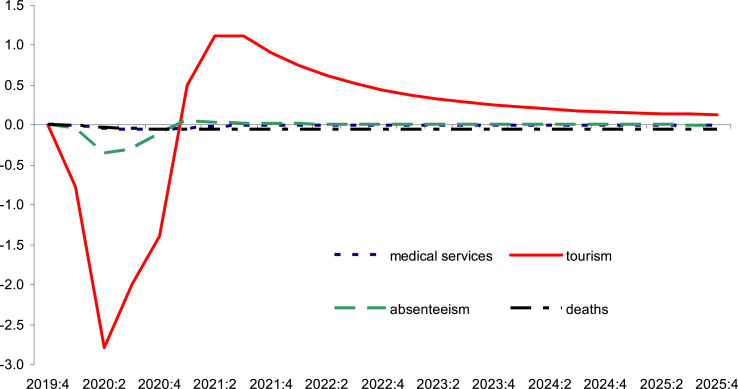
To understand the effects of the four categories of shocks on global GDP, Fig. 7 shows the individual effect of each shock. In 2020, the increase in medical services (due to hospitalisations and treatments), the reductions in labour supply (due to deaths) and labour productivity (due to lost workdays), and the fall in international tourism have negative effects on GDP. Of these shocks, the fall in international tourism dominates; the peak effect here is −2.8%, which accounts for most of the peak GDP effect of −3% in 2020 for all shocks combined. The importance of the tourism effects is also reflected in Fig. 7 as large negative effects on global exports. The effect on exports is dominated by the fall in international travel and tourism due to the pandemic.
Fig. 7.
Global GDP - individual shocks (percentage change).
Fig. 7 shows that the temporary reduction in international tourism dwarfs all other effects. This pandemic has a relatively high global infection rate in historical terms (24%). As discussed earlier, the infection rate is the dominant determinant of the size of the tourism reductions. This characteristic of the pandemic causes the tourism effects of this pandemic to be very large relative to other effects. A pandemic with a much reduced infection rate (e.g., the 1957 pandemic) would be expected to lead to much smaller quarantine-like measures (e.g., social exclusion and travel restrictions) to prevent the spread of the virus, and thus much smaller temporary reductions in tourism.
Beginning in 2021:1, the exogenous shocks representing the pandemic are slowly withdrawn and this process is complete by 2021:4. Thus, Fig. 6 shows GDP and labour move above baseline in 2021:1 by 0.4% and 0.7%. In 2021:2 and 2021:3, GDP and labour continue to move above baseline. This is due to the lagged response of wage rates to the end of the pandemic; this means that real wage rates are still 0.5% below baseline in 2021:4 as they only adjust slowly to the change in labour market conditions. From 2021:1 labour usage and GDP move back towards baseline as real wage rates also move back towards baseline. By 2025 labour and real GDP return close to baseline levels.
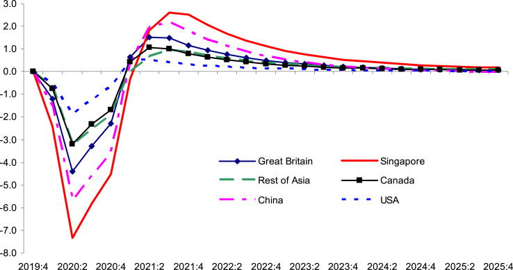
Fig. 8 presents the GDP effects for selected regions. All regions are projected to experience lower output in the short-run (Table 2): the differences across regions are purely due to the size of the negative output effects. Singapore experiences the largest negative deviation in 2020 real GDP: 7.3% in 2020:2. The very large effect on Singapore's GDP is due to the strong negative effect on global trade (exports; see Fig. 7) from the pandemic rather than the direct impact of reduced inbound tourism to Singapore. Singapore is an entrepȏt port through which large volumes of goods and persons pass on the way to their final destination. This is reflected in export and import to GDP shares of around 150% in the base data. This trade is heavily dependent on world trade but even more dependent on trade by Asian regions. As already noted, these regions are the most strongly affected by the influenza outbreak. Thus, Singapore is the region most exposed to the contraction in global and Asian trade due to its unique transit status.
Fig. 8.
GDP effects for selected regions (percentage change).
Other countries with high trade-to-GDP shares also experience a strong negative indirect effect on their GDP due to the contraction in global trade. But the size of international tourism in GDP is also important for determining the GDP effects for other countries. Thus, China (−5.7%), Great Britain (−4.4%), Canada (−3.2%) and Rest of Asia (−3.2%) experience relatively large peak GDP effects (2020:2), whereas USA (−1.9%), Brazil (−1%) and India (−0.7%) experience smaller peak GDP effects.
7. The economic effects of pandemic coronavirus
Here we apply the direct effects of coronavirus to the economic model. These direct effects are orders of magnitude larger than those applied earlier for the influenza pandemic due to the widespread and severe mitigation measures adopted in response to coronavirus. A notable effect of these responses is the extensive underutilisation of physical capital, i.e., capital idling. To account for this phenomenon the economic model is modified to allow for variable capital utilisation; the typical assumption is full capital utilisation. Allowing for capital idling means that large demand-driven reductions in output can be captured in the absence of large reductions in prices or deflation. This imposes consistency in the representation of the capital and labour markets (see section 3.3) in that neither market is assumed to clear on an ongoing basis.
In representing capital idling here the approach follows the treatment in real business cycle models where capital use is typically varied along the intensive margin [25]. Here this is represented formally as
| (7) |
where is the quantity of capital available for use in region r in year t (see (4)) and is the quantity of capital in use. Thus, is the capital utilisation rate. This rate is a positive function of the ratio of the rental price of capital and average supply price for all industries , i.e., the real cost of capital. is positive parameter.
Linearisation of (7) yields where is the proportional change in the capital utilisation rate. Thus, a rising real cost of capital in the current period signals to firms to increase their use of currently idle capital rather than undertake more investment that would lead to more capital in the next period. This means that if the demand for capital falls in a given period, this will be partially reflected as a fall in the rental price of capital and partially as a fall in capital used. Under normal circumstances (full capital utilisation) a fall in the demand for capital would be almost totally reflected as a fall in the rental price, as capital used must equal capital supply (stock), and capital supply can only change slowly due to a one-period gestation lag.
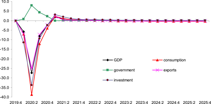
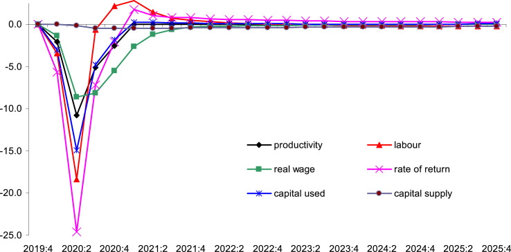
Applying the direct impacts of coronavirus in quarter 1 of 2020 (2020:1) global GDP falls by 5.7%, labour by 3.4% and capital used by 3% (see Fig. 9, Fig. 10 , Table 3 ). This mainly reflects prophylactic behaviour by firms and households in response to rising infections. In 2020:2 the full effects of the virus take hold so that GDP, labour and capital collapse (−27%, −18% and −15%) as new infections continue to rise and almost all countries adopt severe mitigation strategies (see Fig. 5). The contractionary effect of the pandemic reduces demand for labour by firms. As wage rates are rigid in the short-run the real wage rate falls by much less: 1.37% and 8.6% in 2020:1 and 2020:2.
Fig. 9.
Global GDP and expenditure components (percentage change).
Fig. 10.
Global GDP income components (percentage change).
Table 3.
Global and regional GDP (percentage change).
| Region |
Quarter |
|||||||
|---|---|---|---|---|---|---|---|---|
| 2020:1 | 2020:2 | 2020:3 | 2020:4 | 2021:1 | 2021:2 | 2021:3 | 2021:4 | |
| World | −5.69 | −27.37 | −8.13 | −2.43 | 1.84 | 1.01 | 0.55 | 0.38 |
| Australia | −24.94 | −19.31 | 0.00 | 0.45 | 1.41 | 1.01 | 0.78 | 0.67 |
| Rest of Oceania | −15.95 | −21.96 | −0.50 | 0.62 | 1.82 | 1.60 | 1.49 | 1.40 |
| China | −20.06 | −6.31 | 1.94 | 2.20 | 2.18 | 2.14 | 2.11 | 2.02 |
| Japan | −2.20 | −29.08 | −9.29 | −2.59 | 2.34 | 1.16 | 0.40 | 0.13 |
| Korea | −20.50 | −3.84 | 1.29 | 1.86 | 1.87 | 2.42 | 2.38 | 2.26 |
| India | −0.14 | −17.30 | −9.43 | −4.22 | −0.49 | 0.62 | 0.31 | 0.15 |
| Indonesia | −1.64 | −18.08 | −8.33 | −3.31 | 0.19 | 0.70 | 0.37 | 0.20 |
| Singapore | −4.45 | −27.59 | −12.58 | −4.78 | −1.02 | −0.42 | −0.11 | −0.18 |
| Rest of Asia | −2.32 | −22.27 | −10.16 | −3.76 | 0.68 | 0.92 | 0.51 | 0.30 |
| Canada | −2.05 | −29.47 | −10.46 | −3.47 | 1.80 | 0.97 | 0.40 | 0.21 |
| United States | −2.62 | −34.99 | −9.49 | −2.71 | 2.67 | 0.74 | 0.06 | −0.10 |
| Mexico | −0.97 | −19.06 | −8.61 | −3.54 | 1.46 | 0.31 | 0.23 | 0.21 |
| Argentina | −2.68 | −26.88 | −10.79 | −4.01 | 1.06 | 0.71 | 0.43 | 0.29 |
| Brazil | −0.45 | −23.71 | −11.76 | −4.57 | 1.31 | 1.05 | 0.55 | 0.35 |
| Rest of South America | −1.38 | −22.84 | −10.73 | −4.15 | 0.78 | 0.57 | 0.17 | 0.00 |
| France | −7.98 | −31.84 | −7.01 | −1.89 | 2.11 | 0.93 | 0.46 | 0.26 |
| Germany | −9.33 | −30.96 | −6.76 | −1.63 | 2.22 | 1.20 | 0.76 | 0.54 |
| Italy | −8.44 | −21.27 | −8.79 | −3.54 | 0.76 | 0.91 | 0.85 | 0.76 |
| Great Britain | −2.90 | −34.11 | −11.37 | −3.48 | 1.84 | 0.94 | 0.30 | 0.05 |
| Rest of EU | −6.43 | −29.30 | −9.15 | −2.84 | 1.56 | 1.05 | 0.68 | 0.47 |
| Rest Europe | −8.56 | −28.87 | −7.22 | −1.68 | 2.45 | 1.35 | 0.93 | 0.72 |
| Russia | −3.23 | −23.50 | −12.17 | −5.62 | −1.20 | −0.25 | −0.40 | −0.47 |
| Former Soviet Union | −3.54 | −24.17 | −9.82 | −3.25 | 2.22 | 0.55 | 0.17 | −0.02 |
| Turkey | −0.92 | −19.67 | −9.85 | −4.07 | 0.23 | 0.64 | 0.31 | 0.16 |
| Rest of Middle East | −2.53 | −17.81 | −8.14 | −3.57 | −0.42 | 0.37 | 0.32 | 0.31 |
| South Africa | −2.56 | −23.34 | −11.30 | −4.18 | 1.04 | 0.88 | 0.41 | 0.23 |
| Rest of Africa | −1.15 | −15.10 | −7.22 | −3.26 | −0.95 | 0.32 | 0.22 | 0.16 |
In 2020:3 the number of new global infections begins to fall. Despite this, mitigation measures are only relaxed slowly in 2020:3 and 2020:4. Thus global economic activity begins to recover but still remains depressed. As economic activity begins to recover over 2020:3–4 real wage rates respond with a lag to the recovery in labour demand. The delayed response of real wage rates helps clear the excess supply in the labour market and labour usage largely recovers to only 0.6% below baseline in 2020:3 and 2.2% above baseline in 2020:4. GDP recovers much more slowly to be 8.1% and 2.4% below baseline in 2020:3 and 2020:4. The recovery path is similar for capital over 2020:3–4.
In 2021 the shocks representing the pandemic are slowly withdrawn and this process is complete by the end of 2021. Thus, GDP moves above baseline in 2021:1 by 1.8% and labour expands further to 2.8%. By this time the real wage rate has begun to rise and the overshooting that this initially causes in labour usage ends, and from 2020:2 onwards GDP and labour begin to move back towards baseline. By 2021:4 global GDP, labour and capital return close to baseline levels.
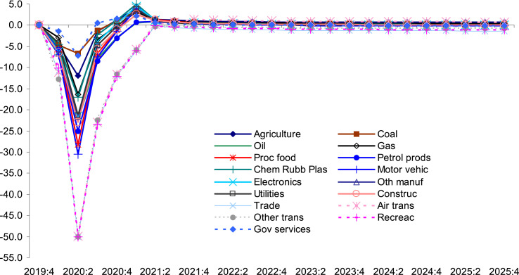
The negative effects on industry output at the global level show a wide variation in effects (Fig. 11 ). These effects peak in 2020:2. The smallest effects are observed for agriculture (−12%), coal (−6.7%), other minerals (−2.2%) and government services (−7.1%). The largest effects are observed for industries directly related to international travel and tourism: wholesale and retail trade, air transport, other transport, and recreation services, all of which contract by around 50% in 2020:2. Most industries recover by 2021:1 except for international travel and tourism; these take until 2021:3 or 2021:4 to recover their output levels.
Fig. 11.
Global industry output (percentage change).
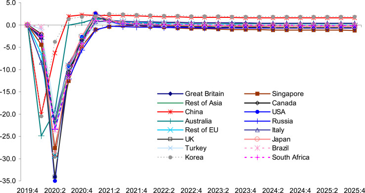
The time path of regional output closely follows that already discussed for global output (Fig. 12 , Table 3). The exceptions are Australia, China and Korea. For China and Korea this is because peak infections occur in 2020:1 and fall thereafter. China is where the virus begins and from there it quickly spread to Japan and Korea. Thus, mitigation measures were implemented very early in these countries. In 2020:2 GDP in China and Korea recovers to be 6.3% and 2.8% below baseline. For Australia GDP is still heavily depressed by 19%. The largest output contractions in 2020:2 are observed in the US (−35%), the UK (−34%), France (−32%), Germany (−31%), Canada (−29%), Japan (−29%), Rest of EU (−29%), Rest of Europe (−29%) and Singapore (−27%). The distribution of these output contractions largely reflects the importance in each regional economy of those industries that experience the largest output contractions, i.e., those closely related to domestic and international and tourism. This is similar to what was observed in the previous section regarding pandemic influenza.
Fig. 12.
Regional GDP (percentage change).
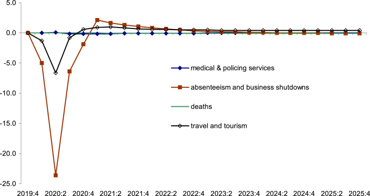
Fig. 13 presents the effect on global GDP of the four categories of direct effects. Similar to the pandemic influenza scenario, the increase in medical and policing services and the reductions in labour supply have marginal impacts relative to absenteeism and business shutdowns and the fall in travel and tourism. In contrast to the influenza scenario, the fall in travel and tourism is less important than absenteeism and business shutdowns; the former has a peak effect of −6.6% whereas the latter has a peak effect of −24%. The strong impact of absenteeism and business shutdowns is driven by the widespread and severe mitigation strategies adopted almost universally during the current pandemic. Many businesses deemed as non-essential have been forced to close as part of widespread social distancing measures.
Fig. 13.
Global GDP - individual shocks(percentage change).
8. Conclusion
Infectious diseases are a leading cause of death worldwide. Previous analysis has demonstrated infectious disease outbreaks can easily cross borders to threaten economic stability. The current outbreak of human coronavirus (COVID-19) is a reminder of this threat. The constant adaptation of microbes, along with their ability to evolve and become resistant to antibacterial and antiviral agents, ensures that infectious diseases will continue to be an ever-present and ever-changing economic threat. Therefore, assessing these threats is important for informing households, governments and businesses on the possible economic disruption from infectious disease outbreaks. The present study compares two pandemic scenarios, one caused by influenza and the other by human coronavirus. Both of these are now a regularly recurring form of infectious disease. The economic effects are assessed by modelling a hypothetical but typical influenza pandemic by linking epidemiological and economic models. The coronavirus scenario is fashioned by drawing on the influenza scenario and data currently available for COVID-19 deaths and infections.
An important feature of these pandemics is their short, sharp nature; they usually begin and end within a year. Hence, in understanding the economic disruption from a pandemic a framework is applied that captures the comparative advantages of both macroeconomic and computable general equilibrium (CGE) models. Macroeconomic models have the advantage of assuming quarterly periodicity that allows them to capture the short, sharp nature of pandemics; they have the disadvantage of a single-sector approach that ignores sectors that are particularly relevant to the study of the economic effects of epidemics. CGE models have the advantage of identifying multiple sectors in the economy; they have the disadvantage of annual periodicity and so are unable to capture accurately the short, sharp nature of influenza pandemics. Here we apply a CGE model incorporating quarterly periodicity.
The influenza and coronavirus scenarios begin in quarter 1 of 2020 (2020:1) and lead to global GDP reductions that peak at −3% and −27% in 2020:2. The influenza scenario leads a recession whereas the coronavirus scenario lead to a global depression. The main reason driving this difference is the widespread and severe mitigation strategies that have been adopted worldwide in response to the coronavirus outbreak. The most detrimental of these is the forced shutdown of non-essential business in order to reduce social contact and transmission of the virus. The measures lead to a large fall in labour productivity as workers are forced to work from home or work under restrictive conditions. From 2020:3 the number of new global infections begins to fall in both scenarios and thus mitigation measures are relaxed slowly in 2020:3 and 2020:4. Thus global economic activity begins to recover but still remains depressed. In both scenarios economic activity begins to recover in 2021:1, overshoots through the year and is close to baseline GDP by the beginning of 2022.
The recovery path for the coronavirus scenario is largely dependent on the rate of new infections following the path observed for most past pandemics; that is, no significant second wave of infections so that the rate of new infections is low by 2020:3 and lower by 2020:4. This is the most probable outcome. Nevertheless, if this historical path is not repeated then economic activity may stay recessed for longer than the one year projected in the analysis here.
Consistent with previous work, the results show that the largest economic impacts of an infectious disease pandemic are driven by reduced travel and tourism, due to risk-modifying measures by households and travel restrictions imposed by health authorities, and lost workdays, due to illness or formal social distancing measures designed to contain the virus. The analysis shows that travel and tourism reductions are more important in the influenza scenario and that lost workdays are more important in the coronavirus scenario. This reflects the severity of the compulsory social distancing measures imposed during the coronavirus scenario. It may also reflect a characteristic of future pandemics if governments were to repeat this strategy during future infectious disease outbreaks. The analysis here suggests that such a strategy comes at a high economic cost and should be applied with caution.
Author statement
I am the sole author of this paper.
Acknowledgements
Thanks are due to Kevin Hanslow and two referees for helpful comments on this paper. Thanks are also due to Marc Mariano for research assistance. The views expressed here are the author's and do not necessarily reflect those of KPMG or Griffith University.
Biography
Dr George Verikios is Director at KPMG Economics and Adjunct Professor in the Department of Accounting, Finance and Economics at Griffith University. He has a broad array of research interests including economywide analysis and forecasting, tax policy, impact analysis, transport policy, tourism policy, infectious and chronic diseases, trade liberalisation, climate change policy, the circular economy and income distribution. Dr Verikios is author or co-author of 25 journal articles.
The World Health Organization does not provide an estimate of the CFR for H1N1. A range of estimates exist from different studies. [27]. review 50 studies that estimated the CFR for H1N1. The highest of these were around 0.1%, which is similar to seasonal influenza.
The model is implemented in GEMPACK [28].
The exceptions are intertemporal models that compute results simultaneously for all time periods, e.g., Ref. [29].
See Ref. [30] for an example of this approach.
See Ref. [31] for a survey of approaches to modelling inertia in investment behaviour.
The GDP data are sourced from the International Monetary Fund's World Economic Outlook Database. The labour supply data are sourced from the International Labour Organization's Labour Statistics Database.
Supplementary data to this article can be found online at https://doi.org/10.1016/j.seps.2020.100898.
The shocks are explained in detail in Ref. [19].
There seem to be only two known exceptions to compulsory social-distancing measures during the coronavirus pandemic: Sweden and Singapore [34].
See Ref. [35] for an extensive list of cancelled events.
See Ref. [14] for a list of travel restrictions by country.
Appendix A. Supplementary data
The following is the Supplementary data to this article:
References
- 1.Dobson A.P., Carper E.R. Infectious diseases and human population history. Bioscience. 1996;46(2):115–126. [Google Scholar]
- 2.Chou J., Kuo N.-F., Peng S.-L. “Potential impacts of the SARS outbreak on taiwan's economy. Asian Econ Pap. 2004;3(1):84–99. [Google Scholar]
- 3.Fan E.X. Asian Development Bank; Manila: 2003. SARS: economic impacts and implications. Economics and research department policy brief series No. 15. [Google Scholar]
- 4.Hai W., Zhao Z., Wang J., Hou Z.-G. The short-term impact of SARS on the Chinese economy. Asian Econ Pap. 2004;3(1):57–61. [Google Scholar]
- 5.Keogh-Brown M.R., Wren-Lewis S., Edmunds W.J., Beutels P., Smith R.D. The possible macroeconomic impact on the UK of an influenza pandemic. Health Econ. 2010;19(11):1345–1360. doi: 10.1002/hec.1554. [DOI] [PubMed] [Google Scholar]
- 6.Verikios G., McCaw J., McVernon J., Harris A. H1N1 influenza and the Australian macroeconomy. J Asia Pac Econ. 2012;17(1):22–51. [Google Scholar]
- 7.Centers for Disease Control and Prevention . 2020. How COVID-19 spreads.https://www.cdc.gov/coronavirus/2019-ncov/prevent-getting-sick/how-covid-spreads.html [PubMed] [Google Scholar]
- 8.Coronaviridae Study Group of the International Committee on Taxonomy of Viruses The species Severe acute respiratory syndrome-related coronavirus: classifying 2019-nCoV and naming it SARS-CoV-2. Nature Microbiology. 2020;5:536–544. doi: 10.1038/s41564-020-0695-z. [DOI] [PMC free article] [PubMed] [Google Scholar]
- 9.Sander B., Nizam A., Garrison L.P., Postma M.J., Halloran M.E., Longini M.S. Economic evaluation of influenza pandemic mitigation strategies in the United States using a stochastic microsimulation transmission model. Value Health. 2009;12(2):226–233. doi: 10.1111/j.1524-4733.2008.00437.x. [DOI] [PMC free article] [PubMed] [Google Scholar]
- 10.United Nations . 2020. WHO Director-General's opening remarks at the media briefing on COVID-19 - 11 March 2020.https://www.who.int/dg/speeches/detail/who-director-general-s-opening-remarks-at-the-media-briefing-on-covid-19---11-march-2020 [Google Scholar]
- 11.Center for Systems Science and Engineering . John Hopkins University; 2020. COVID-19 dashboard.https://gisanddata.maps.arcgis.com/apps/opsdashboard/index.html#/bda7594740fd40299423467b48e9ecf6 [DOI] [PMC free article] [PubMed] [Google Scholar]
- 12.Oke J., Heneghan C. 2020. ‘Global covid-19 case fatality rates’, the centre for evidence-based medicine.https://www.cebm.net/covid-19/global-covid-19-case-fatality-rates March 17 (updated May 12) [Google Scholar]
- 13.Rajgor, D.D., Lee, M.H., Archuleta, S., Bagdasarian, N., Quek, S.C. ‘The many estimates of the COVID-19 case fatality rate’, The lancet: infectious diseases, Correspondence, March 27. [DOI] [PMC free article] [PubMed]
- 14.Salcedo A., Yar S., Cherelus G. New York Times; 2020. Coronavirus travel restrictions, across the globe.https://www.nytimes.com/article/coronavirus-travel-restrictions.html [Google Scholar]
- 15.Beutels P., Edmunds W.J., Smith R.D. Partially wrong? Partial equilibrium and the economic analysis of public health emergencies of international concern. Health Econ. 2008;17(11):1317–1322. doi: 10.1002/hec.1339. [DOI] [PubMed] [Google Scholar]
- 16.James S., Sargent T. Department of Finance; Canada: 2006. The economic impact of an influenza pandemic. Working paper 2007-04. [Google Scholar]
- 17.Keogh-Brown M.R., Smith R.D. The economic impact of SARS: how does the reality match the predictions? Health Pol. 2008;88(1):110–120. doi: 10.1016/j.healthpol.2008.03.003. [DOI] [PMC free article] [PubMed] [Google Scholar]
- 18.Gopinath G. IMFBlog; 2020. ‘The Great lockdown: worst economic downturn since the Great depression’.https://blogs.imf.org/2020/04/14/the-great-lockdown-worst-economic-downturn-since-the-great-depression [Google Scholar]
- 19.Verikios G. Department of Accounting, Finance and Economics, Griffith University; 2017. The importance of periodicity in modelling infectious disease outbreaks. Discussion paper No. 2017-11. Economics and business Statistics. [Google Scholar]
- 20.Narayanan B.G., Walmsley T.L., editors. Global trade, assistance, and production: the GTAP 7 data base. Center for global trade analysis. Purdue University; 2008. [Google Scholar]
- 21.Bargain O., Orsini K., Peich A. Institute for the Study of Labor; Bonn: 2011. Labor supply elasticities in Europe and the US. IZA discussion paper No. 5820. [Google Scholar]
- 22.Romer D. second ed. McGraw-Hill; Boston: 2001. Advanced macroeconomics. [Google Scholar]
- 23.Verikios G., Sullivan M., Stojanovski P., Giesecke J., Woo G. Monash University; 2011. The global economic effects of pandemic influenza. General paper No. G-224. Centre of policy studies. [Google Scholar]
- 24.Roser M., Ritchie H., Ortiz-Ospina E., Hasell J. 2020. Coronavirus pandemic (COVID-19)https://ourworldindata.org/coronavirus [Google Scholar]
- 25.King R.G., Rebelo S.T. “Resuscitating real business cycles'. In: Taylor J.B., Woodford M., editors. Handbook of macroeconomics. Elsevier North Holland; Amsterdam: 1999. pp. 927–1007. [Google Scholar]
- 26.World Health Organization . Changing History; Geneva: 2004. Global health report 2004. [Google Scholar]
- 27.Wong J., Kelly H., Ip D.K., Wu J., Leung G., Cowling B. Case fatality risk of influenza A (H1N1pdm09): a systematic review. Epidemiology. 2013;24(6):830–841. doi: 10.1097/EDE.0b013e3182a67448. [DOI] [PMC free article] [PubMed] [Google Scholar]
- 28.Harrison W.J., Pearson K.R. Computing solutions for large general equilibrium models using GEMPACK. Comput Econ. 1996;9(2):83–127. [Google Scholar]
- 29.McKibbin W.J., Wilcoxen P.J. The theoretical and empirical structure of the G-cubed model. Econ Modell. 1999;16(1):123–148. [Google Scholar]
- 30.Kouparitsas M.A. vols. 98–15. Federal Reserve Bank of Chicago; Chicago: 1998. Dynamic trade liberalization analysis: steady state, transitional and inter-industry effects. (Working paper WP). [Google Scholar]
- 31.Chirinko R.S. Business fixed investment spending: modeling strategies, empirical results, and policy implications. J Econ Lit. 1993;XXXI(Dec.):1875–1911. [Google Scholar]
- 32.Jonung L., Roeger W. European Commission, Directorate-General for Economic and Financial Affairs; 2006. The macroeconomic effects of a pandemic in Europe: a model-based assessment. European economy economic papers No. 251. [Google Scholar]
- 33.McKibbin W.J., Sidorenko A.A. Lowy Institute for International Policy; 2006. Global macroeconomic consequences of pandemic influenza. [Google Scholar]
- 34.Townsend A. MedicineNet; 2020. Sweden and Singapore: the COVID-19 'soft' approach vs. Techno-surveillance.https://www.medicinenet.com/script/main/art.asp?articlekey=230288 April 14. [Google Scholar]
- 35.New York Times . New York Times; 2020. ‘A list of what's been canceled because of the coronavirus'.https://www.nytimes.com/article/cancelled-events-coronavirus.html [Google Scholar]
Associated Data
This section collects any data citations, data availability statements, or supplementary materials included in this article.


